{hhsong, khatz, vacha, yzhang, lili}@cs.utexas.edu. ABSTRACT. Proximity ... proximity measures in online social networks due to their massive scale (with ..... We consider three classes of proximity measures summarized in. Table 1, which are ...
Scalable Proximity Estimation and Link Prediction in Online Social Networks Han Hee Song
Tae Won Cho
Vacha Dave
Yin Zhang
Lili Qiu
The University of Texas at Austin
{hhsong, khatz, vacha, yzhang, lili}@cs.utexas.edu
ABSTRACT
1. INTRODUCTION
Proximity measures quantify the closeness or similarity between nodes in a social network and form the basis of a range of applications in social sciences, business, information technology, computer networks, and cyber security. It is challenging to estimate proximity measures in online social networks due to their massive scale (with millions of users) and dynamic nature (with hundreds of thousands of new nodes and millions of edges added daily). To address this challenge, we develop two novel methods to efficiently and accurately approximate a large family of proximity measures. We also propose a novel incremental update algorithm to enable near real-time proximity estimation in highly dynamic social networks. Evaluation based on a large amount of real data collected in five popular online social networks shows that our methods are accurate and can easily scale to networks with millions of nodes. To demonstrate the practical values of our techniques, we consider a significant application of proximity estimation: link prediction, i.e., predicting which new edges will be added in the near future based on past snapshots of a social network. Our results reveal that (i) the effectiveness of different proximity measures for link prediction varies significantly across different online social networks and depends heavily on the fraction of edges contributed by the highest degree nodes, and (ii) combining multiple proximity measures consistently yields the best link prediction accuracy.
A social network [53] is a social structure modeled as a graph, where nodes represent people or other entities embedded in a social context, and edges represent specific types of interdependency among entities, e.g., values, visions, ideas, financial exchange, friendship, kinship, dislike, conflict or trade. Understanding the nature and evolution of social networks has important applications in a number of fields such as sociology, anthropology, biology, economics, information science, and computer science. Traditionally, studies on social networks often focus on relatively small social networks (e.g., [30, 31] examine co-authorship networks with about 5000 nodes). Recently, however, social networks have gained tremendous popularity in the cyber space. Online social networks such as MySpace [40], Facebook [18] and YouTube [55] have each attracted tens of millions of visitors every month [44] and are now among the most popular sites on the Web [4]. The wide variety of online social networks and the vast amount of rich information available in these networks represent an unprecedented research opportunity for understanding the nature and evolution of social networks at massive scale. A central concept in the computational analysis of social networks is proximity measure, which quantifies the closeness or similarity between nodes in a social network. Proximity measures form the basis for a wide range of important applications in social and natural sciences (e.g., modeling complex networks [6, 13, 25, 42]), business (e.g., viral marketing [23], fraud detection [11]), information technology (e.g., improving Internet search [35], collaborative filtering [7]), computer networks (e.g., constructing overlay networks [45]), and cyber security (e.g., mitigating email spams [22], defending against Sybil attacks [56]). Unfortunately, the explosive growth of online social networks imposes significant challenges on proximity estimation. First, online social networks are typically massive in scale. For example, MySpace has over 400 million user accounts [41], and Facebook has reportedly over 120 million active users world wide [19]. As a result, many proximity measures that are highly effective in relatively small social networks (e.g., the classic Katz measure [26]) become computationally prohibitive in large online social networks with millions of nodes [48]. Second, online social networks are often highly dynamic, with hundreds of thousands of new nodes and millions of edges added daily. In such fast-evolving social networks, it is challenging to compute up-to-date proximity measures in a timely fashion.
Categories and Subject Descriptors H.3.5 [Information Storage and Retrieval]: Online Information Services—Web-based services; J.4 [Computer Applications]: Social and Behavioral Sciences—Sociology
General Terms Algorithms, Human Factors, Measurement
Keywords Social Network, Proximity Measure, Link Prediction, Embedding, Matrix Factorization, Sketch
Permission to make digital or hard copies of all or part of this work for personal or classroom use is granted without fee provided that copies are not made or distributed for profit or commercial advantage and that copies bear this notice and the full citation on the first page. To copy otherwise, to republish, to post on servers or to redistribute to lists, requires prior specific permission and/or a fee. IMC’09, November 4–6, 2009, Chicago, Illinois, USA. Copyright 2009 ACM 978-1-60558-770-7/09/11 ...$10.00.
Approach and contributions. To address the above challenges, we develop two novel techniques, proximity sketch and proximity embedding, for efficient and accurate proximity estimation in large social networks with millions of nodes. We then augment these techniques with a novel incremental proximity update algorithm to enable near real-time proximity estimation in highly dynamic
social networks. Our techniques are applicable to a large family of commonly used proximity measures, which includes the aforementioned Katz measure [26], as well as rooted PageRank [30, 31] and escape probability [50]. These proximity measures are known to be highly effective for many applications [30, 31, 50], but were previously considered computationally prohibitive for large social networks [48, 50]. To demonstrate the practical value of our techniques, we consider a significant application of proximity estimation: link prediction, which refers to the task of predicting the edges that will be added to a social network in the future based on past snapshots of the network. As shown in [30, 31], proximity measures lie right at the heart of link prediction. Understanding which proximity measures lead to the most accurate link predictions provides valuable insights into the nature of social networks and can serve as the basis for comparing various network evolution models (e.g., [6, 13, 25, 42]). Accurate link prediction also allows online social networks to automatically make high-quality recommendations on potential new friends, making it much easier for individual users to expand their social neighborhood. We evaluate the effectiveness of our proximity estimation methods using a large amount of real data collected in five popular online social networks: Digg [14], Flickr [20], LiveJournal [33], MySpace [40], and YouTube [55]. Our results show that our methods are accurate and can easily scale to handle large social networks with millions of nodes and hundreds of millions of edges. We also conduct extensive experiments to compare the effectiveness of a variety of proximity measures for link prediction in these online social networks. Our results uncover two interesting new findings: (i) the effectiveness of different proximity measures varies significantly across different networks and depends heavily on the fraction of edges contributed by the highest degree nodes, and (ii) combining multiple proximity measures using an off-the-shelf machine learning software package consistently yields the best link prediction accuracy. Paper organization. The rest of the paper is organized as follows. In Section 2, we develop techniques to efficiently and accurately approximate a large family of proximity measures in massive, dynamic online social networks. In Section 3, we describe link prediction techniques. In Section 4, we evaluate both proximity estimation and link prediction in five popular online social networks. In Section 5, we review related work. We conclude in Section 6.
2.
SCALABLE PROXIMITY ESTIMATION
Proximity measures are the basis for many applications of social networks. As a result, a variety of proximity measures have been proposed. The simplest proximity measures are based on either the shortest graph distance or the maximum information flow between two nodes. One can also define proximity measures based on node neighborhoods (e.g., the number of common neighbors). Finally, several more sophisticated proximity measures involve infinite sums over the ensemble of all paths between two nodes (e.g., Katz measure [26], rooted PageRank [30, 31], and escape probability [50]). Compared with more direct proximity measures such as shortest graph distances and numbers of shared neighbors, pathensemble based proximity measures capture more information about the underlying social structure and have been shown to be more effective in social networks with thousands of nodes [30, 31, 50]. Despite the effectiveness of path-ensemble based proximity measures, it is computationally expensive to summarize the ensemble of all paths between two nodes. The state of the art in estimating path-ensemble based proximity measures (e.g., [50]) typically can only handle social networks with tens of thousands of nodes. As a result, recent works on proximity estimation in large social
networks (e.g., [48]) either dismiss path-ensemble based proximity measures due to their prohibitive computational cost or leave it as future work to compare with these proximity measures. In this section, we address the above challenge by developing efficient and accurate techniques to approximate a large family of path-ensemble based proximity measures. Our techniques can handle social networks with millions of nodes, which are several orders of magnitude larger than what the state of the art can support. In addition, our techniques can support near real-time proximity estimation in highly dynamic social networks.
2.1 Problem Formulation Below we first formally define three commonly used path-ensemble based proximity measures: (i) Katz measure, (ii) rooted PageRank, and (iii) escape probability. We then show that all three proximity measures can be efficiently estimated by solving a common subproblem, which we term the proximity inversion problem. In all our discussions below, we model a social network as a graph G = (V, E), where V is the set of nodes, and E is the set of edges. G can be either undirected or directed, depending on whether the social relationship is symmetric. Katz measure. The Katz measure [26] is a classic path-ensemble based proximity measure. It is designed to capture the following simple intuition: the more paths there are between two nodes and the shorter these paths are the stronger the relationship is (because there are more opportunities for the two nodes to discover and interact with each other in the social network). Given two nodes x, y ∈ V , the Katz measure Katz[x, y] is a weighted sum of the number of paths from x to y, exponentially damped by length to count short paths more heavily. Formally, we have Katz[x, y] =
∞ X
ℓ βKatz · |pathshℓi x,y |
(1)
ℓ=1
where pathshℓi x,y is the set of length-ℓ paths from x to y, and βKatz is a damping factor. Let A be the adjacency matrix of graph G, where 1, if hx, yi ∈ E, A[x, y] = (2) 0, otherwise. As shown in [31], the Katz measures between all pairs of nodes (represented as a matrix Katz) can be derived as a function of the adjacency matrix A and the damping factor βKatz as follows: Katz =
∞ X
ℓ βKatz Aℓ = (I − βKatz A)−1 − I
(3)
ℓ=1
where I is the identity matrix. Thus, in order to compute Katz, we just need to compute the matrix inverse (I − βKatz A)−1 . Rooted PageRank. The rooted PageRank [30, 31] is a special instance of personalized PageRank [8,12]. It defines a random walk on the underlying graph G = (V, E) to capture the probability for two nodes to run into each other and uses this probability as an indicator of the node-to-node proximity. Specifically, given two nodes x, y ∈ V , the rooted PageRank RPR[x, y] is defined as the stationary probability of y under the following random walk: (i) with probability 1−βRPR , jump to node x, and (ii) with probability βRPR , move to a random neighbor of current node. The rooted PageRank between all node pairs (represented as a matrix RPR) can beP derived as follows. Let D be a diagonal matrix with D[i, i] = j A[i, j]. Let T = D−1 A be the adjacency matrix with row sums normalized to 1. We then have: RPR = (1 − βRPR )(I − βRPR T )−1
(4)
Therefore, to compute RPR, we just need to compute the matrix inverse (I − βRPR T )−1 . Also note that the standard PageRank can be computed simply as the average of all the columns of RPR. Escape probability. The escape probability [50] is another pathensemble based proximity measure. Given two nodes x, y ∈ V , the escape probability EP[x, y] from x to y is defined as the probability that a random walk which starts from node x will visit node y before it returns to node x [16]. The escape probability EP[x, y] can be directly derived from the rooted PageRank as follows. EP[x, y] =
Q[x, y] Q[x, x]Q[y, y] − Q[x, y]Q[y, x]
(5)
where matrix Q = RPR/(1 − βRPR ) = (I − βRPR T )−1 . As shown in [16], when the underlying graph G = (V, E) is undirected, the escape probability EP is also closely related to several other random walk induced proximity or distance measures: effective conductance EC, effective resistance ER, and commute time CT. Specifically, we have: EC[x, y] = ER[x, y] = CT[x, y] =
|N (x)| · EP[x, y] 1/EC[x, y] 2 · |E| · ER[x, y]
(6) (7) (8)
The common subproblem: proximity inversion. From the above discussions, it is evident that the key to estimating all three pathensemble based proximity measures is to efficiently compute elements of the following matrix inverse: △
P = (I − βM )−1 =
∞ X
βℓ M ℓ
(9)
ℓ=0
where M is a sparse nonnegative matrix with millions of rows and columns, I is an identity matrix of the same size, and β ≥ 0 is a damping factor. We term this common subproblem the proximity inversion problem.
2.2 Scalable Proximity Inversion The key challenge in solving the proximity inversion problem (i.e., computing elements of matrix P = (I − βM )−1 ) is that while M is a sparse matrix, P is a dense matrix with millions of rows and columns. It is thus computationally prohibitive to compute and/or store the entire P matrix. To address the challenge, we first develop two novel dimensionality reduction techniques to approximate elements of P = (I − βM )−1 based on a static snapshot of M : proximity sketch and proximity embedding. We then develop an incremental proximity update algorithm to approximate elements of P in an online setting when M continuously evolves.
2.2.1 Preparation
Sk[x,gk(y)] +=P[x,y]
P[x,y]
Pm x m
Sk
Figure 1: Proximity sketch P Similarly, to compute the sum of a subset of rows i∈S P [i, ∗], we first construct an indicator row vector u such that u[i] = 1 for ∀i ∈ P S and u[j] = 0 for ∀j 6∈ S. We then approximate the sum of rows i∈S P [i, ∗] = u P as: u P = u (I − βM )−1 =
∞ X
βℓu M ℓ ≈
ℓ=0
ℓX max
βℓu M ℓ
(11)
ℓ=0
In one extreme where S contains all the column indices, we can compute the sum of all columns in P . This is useful for computing the PageRank (which is the average of all columns in the RPR matrix). In the other extreme where S contains only one element, we can efficiently approximate a single row or column of P . Complexity. Suppose M is an m-by-m matrix with n non-zeros. Computing the product of sparse matrix M and a dense vector v takes O(n) time by exploiting the sparseness of M . So it takes O(n · ℓmax ) time to compute {M ℓ v | ℓ = 1, . . . , ℓmax } and approximate P v. Note that the time complexity is independent of the size of the subset S. The complexity for computing uP is identical. Note however that the above approximation algorithm is not efficient for estimating individual elements of P . In particular, even if we only want a single element P [x, y], we have to compute either a complete row P [x, ∗] or a complete column P [∗, y] in order to obtain an estimate of P [x, y]. So we only apply the above technique for preprocessing. We will develop several techniques in the rest of this section to estimate individual elements of P efficiently. Benefits of truncation. WePachieve two key benefits by trunℓ ℓ cating the infinite expansion ∞ ℓ=0 β M to form a finite expanPℓmax ℓ ℓ sion ℓ=0 β M . First, we completely eliminate the influence of paths with length above ℓmax on the resulting sums. This is desirable because as pointed out in [30,31], proximity measures that are unable to limit the influence of overly lengthy paths tend to perform P max ℓ ℓ β M is poorly for link prediction. Second, we ensure that ℓℓ=0 P∞ ℓ ℓ always finite, whereas elements of ℓ=0 β M may reach infinity when the damping factor β is not small enough.
2.2.2 Proximity Sketch
We first present an algorithm to approximate the sum of a subset of rows or columns of P = (I − βM )−1 efficiently and accurately. We use this algorithm as a basic building block in both proximity sketch and proximity embedding. Algorithm. P Suppose we want to compute the sum of a subset of columns: i∈S P [∗, i], where S is a set of column indices. We first construct an indicator column vector v such that v[i] = 1 for ∀i ∈ S and v[j] = 0 for ∀j 6∈ S. The sum of columns P i∈S P [∗, i] is simply P v and can be approximated as: P v = (I − βM )−1 v =
P[x,y] is hashed into entry Sk [x,gk (y)] in each hash table Sk (k=1, ..., H) So Sk [x,g k(y)] gives an upper bound on P[x,y] Estimate P[x,y] by taking the min upper bound in all H hash tables
∞ X ℓ=0
βℓM ℓ v ≈
ℓX max
βℓM ℓ v
(10)
ℓ=0
where ℓmax bounds the maximum length of the paths over which the summation is performed.
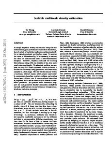
Our first dimensionality reduction technique, proximity sketch, exploits the mice-elephant phenomenon that frequently arises in matrix P in practice, i.e., most elements in P are tiny (i.e., mice) but few elements are huge (i.e., elephants). Algorithm. Figure 1 shows the data structure for our proximity sketch, which consists of H hash tables: S1 , · · · , SH . Each Sk is a 2-dimensional array with m rows and c ≪ m columns. A column hash function gk : {1, · · · , m} → {1, · · · , c} is used to hash each element in Pm×m (P [x, y]) into an element in Sk m×c (Sk [x, gk (y)]). We ensure that different hash functions gk (·) (k = 1, · · · , H) are two-wise independent. In each Sk , each element P [x, y] is added to entry Sk [x, gk (y)]. Thus, X P [a, y] (12) Sk [a, b] = y: gk (y)=b
Probabilistic accuracy guarantee. Our proximity sketch effectively summarizes each row of P : P [x, ∗] using a count-min sketch [10]: {Sk [x, ∗] | k = 1, · · · , H}. As a result, we provide the same probabilistic accuracy guarantee as the count-min sketch, which is summarized in the following theorem (see [10] for detailed proof).
x: fk (x)=a
and store {Rk } (instead of P {Sk }) as thePfinal proximity sketch. Clearly, we have Rk [a, b] = x: fk (x)=a y: gk (y)=b P [x, y]. For any x, y ∈ V , we can then estimate P [x, y] as Pˆ [x, y] = min Rk [fk (x), gk (y)] k
(15)
2.2.3 Proximity Embedding Our second dimensionality reduction technique, proximity embedding, applies matrix factorization to approximate P as the product of two rank-r factor matrices U and V : Pm×m ≈ Um×r · Vr×m
(16)
In this way, with O(2 m r) total state for factor matrices U and V , we can approximate any P [x, y] in O(r) time as: Pˆ [x, y] =
r X
U [x, k] · V [k, y]
Our technique is motivated by recent research on embedding network distance (e.g., end-to-end round-trip time) into low-dimensional space (e.g., [32, 34, 43, 49]). Note however that proximity is the opposite of distance — the lower the distance the higher the proximity. As a result, techniques effective for distance embedding do not necessarily work well for proximity embedding. Algorithm. As shown in Figure 2(a), our goal is to derive the two rank-r factor matrices U and V based on only a subset of rows P [L, ∗] and columns P [∗, L], where L is a set of indices (which we term the landmark set). We achieve this goal by taking the following five steps: 1. Randomly select a subset of ℓ nodes as the landmark set L. The probability for a node i to be included in L is proportional to the PageRank of node i in the underlying graph1 . Note that 1
P[L,L]
We also consider uniform landmark selection, but it yields worse accuracy than PageRank based landmark selection (see Section 4).
V
~
*
P
U
V[*,L]
P[*,L]
~
U
*
V[*,L]
(b) factorize P[L,L] to get U[L,*], V[*,L]
(c) obtain U from P[*,L] and V[*,L]
P[L,*]
~
*
V
(d) obtain V from P[L,*] and U[L,*]
Figure 2: Proximity embedding the PageRank for all the nodes can be precomputed efficiently using the finite expansion method in Section 2.2.1. 2. Compute sub-matrices P [L, ∗] and P [∗, L] efficiently by computing each row P [i, ∗] and each column P [∗, i] (i ∈ L) separately as described in Section 2.2.1. 3. As shown in Figure 2(b), apply singular value decomposition (SVD) to obtain the best rank-r approximation of P [L, L]: P [L, L] ≈ U [L, ∗] · V [∗, L]
(18)
4. Our goal is to find U and V such that U · V is a good approximation of P . As a result, U · V [∗, L] should be a good approximation of P [∗, L]. We can therefore find U such that U · V [∗, L] best approximates sub-matrix P [∗, L] in least-squares sense (shown in Figure 2(c)). Given the use of SVD in step 3, the best U is simply U = P [∗, L] · V [∗, L]T
(19)
5. Similarly, find V such that U [L, ∗] · V best approximates submatrix P [L, ∗] in least-squares sense (shown in Figure 2(d)), which is simply V = U [L, ∗]T · P [L, ∗]
(17)
k=1
V[*,L]
*
P[*,L]
(13)
T HEOREM 1. With H = ⌈ln 1δ ⌉ hash tables, each with c = ⌈ ǫe ⌉ columns, the estimate Pˆ [x, y] guarantees: (i) P [x, y] ≤ Pˆ [x, y]; ˆ and P (ii) with probability at least 1 − δ, P [x, y] ≤ P [x, y] + ǫ · z P [x, z]. P Therefore, as long as P [x, y] is much larger than ǫ · z P [x, z], the relative error of Pˆ [x, y] is small with high probability. Extension. If desired, we can further reduce the space requirement of proximity sketch by aggregating the rows of Sk (at the cost of lower accuracy). Specifically, we associate each Sk with a row hash function fk (·). We then compute X Sk [x, b] (14) Rk [a, b] =
~
U[L,*]
k
P[L,*]
U[L,*]
Pˆ [x, y] = min Sk [x, gk (y)]
P[L,L]
U[L,*]
(a) goal: approximate P as the product of two rank−r matrices U, V by only computing a subset of rows P[L,*] and columns P[*,L]
P Note that each column of Sk : Sk [∗, b] = y:gk (y)=b P [∗, y] can be computed efficiently as described in Section 2.2.1. Since P is a nonnegative matrix, for any x, y ∈ V and any k ∈ [1, H], Sk [x, gk (y)] is an upper bound for P [x, y] according to Eq. 12. We can therefore estimate P [x, y] by taking the minimum upper bound in all H hash tables in O(H) time. That is:
(20)
Accuracy. Unlike proximity sketch, proximity embedding does not provide any provable data-independent accuracy guarantee. However, as a data-adaptive dimensionality reduction technique, when matrix P is in fact low-rank (i.e., having good low-rank approximations), proximity embedding has the potential to achieve even better accuracy than proximity sketch. Our empirical results in Section 4 suggest that this is indeed the case for the Katz measure.
2.2.4 Incremental Proximity Update To enable online proximity estimation, we periodically checkpoint M and use the above dimensionality reduction techniques to approximate P for the last checkpoint of M . Between two checkpoints, we apply an incremental update algorithm to approximate P ′ = (I − β · M ′ )−1 , where M ′ = M + ∆ is the current matrix. Our algorithm is based on the second-order approximation of P ′ : P′
= [I − β(M + ∆)]−1 ≈ (I − βM )−1 + β ∆ + β 2 (∆M + M ∆ + ∆2 )
(21)
The second-order approximation works well as long as ∆ has only few non-zero elements and β is small, making higher order terms negligible. To estimate an individual element P ′ [x, y], we simply use: X 2 β ∆[x, k]M [k, y]+ P ′ [x, y] ≈ P [x, y] + β∆[x, y] +
graph distance common neighbors Adamic/Adar preferential attachment PageRank product
k: ∆[x,k]6=0
X
2
β M [x, k]∆[k, y] +
k: ∆[k,y]6=0
X
β 2 ∆[x, k]∆[k, y]
(22)
k: ∆[x,k]6=0
If we checkpoint M frequently enough, the difference between the last checkpoint M and the current matrix M ′ will be quite small. In other words, the difference matrix ∆ is likely to be sparse. As a result, we expect row ∆[x, ∗] and column ∆[∗, y] to have few non-zero elements. By leveraging such sparseness, we can efficiently compute Eq. 22 in an online fashion. We demonstrate the efficiency and accuracy of our incremental proximity update algorithm in Section 4.2.3.
3.
LINK PREDICTION TECHNIQUES
We use link prediction as a significant application of our proximity estimation methods. Our goal is to understand (i) the effectiveness of various proximity measures in the context of link prediction, and (ii) the benefit of combining multiple proximity measures. In this section, we summarize the link predictors and the proximity measures we use.
3.1 Link Predictors We consider two types of link predictors: (i) basic link predictor that uses a single proximity measure, and (ii) composite link predictor that uses multiple proximity measures. Basic link predictors. A basic link predictor consists of a proximity measure prox[∗, ∗], and a threshold T . Given an input graph G = (V, E) (which models a past snapshot of a given social network), a node pair hx, yi 6∈ E is predicted to form an edge in the future if and only if the proximity between x and y is sufficiently large, i.e., prox[x, y] ≥ T . Composite link predictors. A composite link predictor uses machine learning techniques to make link predictions based on multiple proximity measures. We use the WEKA machine learning package [21] to automatically generate composite link predictors using a number of machine learning algorithms, including the REPtree decision tree learner, J48 decision tree learner, JRip rule learner, support vector machine (SVM) learner, and Adaboost learner. The results are consistent across different learners we use. So we only report the results of the REPtree decision tree learner. REPtree is a variant of the commonly used C4.5 decision tree learning algorithm [46]. It builds a decision tree using information gain and prunes it using reduced error pruning. It allows direct control on the depth of the learned decision tree, making it easy to visualize and interpret the resulting composite link predictor.
3.2 Proximity Measures We consider three classes of proximity measures summarized in Table 1, which are based on (i) graph distance, (ii) node neighborhood, and (iii) ensemble of paths, respectively. Notations. We model a social network as a graph G = (V, E), where V is the set of nodes, and E is the set of edges. G can be either directed or undirected. For a node x, let N (x) = {y|hx, yi ∈ E} be the set of neighbors x has in G. Similarly, let N −1 (x) = {y|hy, xi ∈ E} be the set of inverse neighbors x has in G (i.e., nodes that have x as their neighbors). Let A be the adjacency matrix for G (defined in Eq. 2). Let T = D−1 A be the adjacency
Katz
GD[x, y] = negated distance of the shortest path from x to y CN[x, y] = |N (x) ∩ N (y)| P 1 AA[x, y] = z∈N(x)∩N(y) log |N(z)| PA[x, y] = |N (x)| · |N (y)| PRP[x, y] = P R(x) · P R(y), where P P R(z) P R(x) = 1−d + d z∈N −1 (x) |N(x)| |V | P∞ hℓi ℓ Katz[x, y] = ℓ=1 β · |pathsx,y | we have: Katz = (I − βA)−1 − I
Table 1: Summary of proximity measures matrix with row sums P normalized to 1, where D is a diagonal matrix with D[i, i] = j A[i, j]. Graph distance based proximity measure. Perhaps the most direct metric for quantifying how close two nodes are is the graph distance. We thus define a proximity measure GD[x, y] as the negative of the shortest-path distance from x to y. Note that the use of negated (instead of original) shortest-path distance ensures that the proximity measure GD[x, y] increases as x and y get closer. Note that it is inefficient to apply Dijkstra’s algorithm to compute shortest path distance from x to y when G has millions of nodes. Instead, we exploit the small-world property [27] of the social network and apply expanded ring search to compute the shortest path distance from x to y. Specifically, we initialize S = {x} and D = {y}. In each step we either expand set S to include its members’ neighbors (i.e., S = S ∪ {v|hu, vi ∈ E ∧ u ∈ S}) or expand set D to include its members’ inverse neighbors (i.e., D = D ∪ {u|hu, vi ∈ E ∧ v ∈ D}). We stop whenever S ∩ D 6= ∅ — the number of steps taken so far gives the shortest path distance. For efficiency, we always expand the smaller set between S and D in each step. We also stop when a maximum number of steps is reached (set to 6 in our evaluation). Node neighborhood based proximity measures. We define four proximity measures based on node neighborhood. • Common neighbors. For two nodes x and y, they are more likely to become friends when the overlap of their neighborhoods is large. The simplest form of this approach is to count the size of the intersection: CN[x, y] = |N (x) ∩ N (y)|. • Adamic/Adar. Like common neighbors, Adamic/Adar [1] also tries to measure the size of the intersection of two neighborhoods. However, Adamic/Adar also takes ”rareness” into account, giving more weights to the smaller P common node with 1 number of friends: AA[x, y] = z∈N(x)∩N(y) log |N(z)| . • Preferential attachment. The preferential attachment is based on the idea that having a new neighbor is proportional to the size of the current neighborhood. Moreover, the probability of two users becoming friends is proportional to the product of the number of the current friends. We therefore define a proximity measure: PA[x, y] = |N (x)| · |N (y)|.
• PageRank product. PageRank is developed to analyze the hyperlink structure of Web pages by treating a hyperlink as a vote. The PageRank of a node depends on the count of inbound links and the PageRank of outbound neighbors. Formally, the PageRank of a node x, denoted as P R(x), is defined recursively on G = (V, E) as X P R(z) 1−d P R(x) = +d (23) |V | |N (x)| −1 z∈N
(x)
where d is a damping factor. We define the PageRank product of two nodes x and y as the product of two PageRank values: PRP[x, y] = P R(x) · P R(y).
Path-ensemble based proximity measures. We use the Katz measure (Katz[x, y]) as a path-ensemble based proximity measure (described in Section 2.1). We use the Katz measure as the representative of path-ensemble based proximity measures for two main reasons. First, as shown in [30, 31], the Katz measure is the more effective than other path-ensemble based proximity measures such as the rooted PageRank. Second, our results in Section 4 show that the accuracy of our proximity estimation methods is the highest for the Katz measure.
4.
EVALUATION
4.1 Dataset Description Snapshot # of Conn# of # of Added Asymmetric Date ected Nodes Links Links Link Fraction 9/15/2008 535,071 4,432,726 – 10/25/2008 567,771 4,813,668 656,478 58.3% 11/10/2008 567,771 4,941,401 175,958 Flickr 3/01/2007 1,932,735 26,702,209 – 4/15/2007 2,172,692 30,393,940 3,691,731 37.8% 5/18/2007 2,172,692 32,399,243 2,005,303 Live11/13/2008 1,769,493 61,488,262 – Journal 12/05/2008 1,769,543 61,921,736 1,566,059 28.3% 1/30/2009 1,769,543 62,843,995 3,093,064 MySpace 12/11/2008 2,128,945 89,138,628 – 1/11/2009 2,137,773 90,629,452 1,845,898 0% 2/14/2009 2,137,773 89,341,780 696,016 YouTube 4/30/2007 2,012,280 9,762,825 – 6/15/2007 2,532,050 13,017,064 3,254,239 0% 7/23/2007 2,532,050 15,337,226 2,320,162 Wikipedia 9/30/2006 1,636,961 28,950,137 – 12/31/2006 1,758,323 33,974,708 5,024,571 83.1% 4/06/2007 1,758,323 38,349,329 4,374,621 Network Digg
Table 2: Dataset summary We carry out our evaluation on five popular online social networks: Digg [14], Flickr [20], LiveJournal [33], MySpace [40], and YouTube [55]. For comparison, we also examine the hyperlink structure of Wikipedia [54]. For each network, we conduct three crawls and make three snapshots of the network. Table 2 summarizes the characteristics of the three snapshots for each of the networks. Note that, for the purpose of link prediction, we only use connected nodes (i.e., nodes with at least one incoming or outgoing friendship link), rather than considering all the crawled nodes. Another point to note is that since link prediction implies that based on one snapshot of the network, we predict the new links that are formed in the next snapshot, the same set of users should appear in two consecutive snapshots. Hence, for a growing network, the number of users appearing in the last snapshot that we create may be less than the total number of users (to match the previous snapshot). Lastly, although there can be both link additions and deletions between two snapshots, since the goal of link prediction is to predict those that get added, we explicitly show the number of added links between two consecutive snapshots in Table 2. Digg [14] is a website for users to share interesting Web content by posting a link to it. The posted link can be voted as either positive (“digg”) or negative (“bury”) by other users. Digg allows a user to become a “fan” of other users, which we consider as a friendship relation. All the friendship links together form a directed social graph. Overall, 58.3% directly connected user pairs in Digg have asymmetric friendship (i.e., friendship link only exists in one direction between two users). We obtained the entire list of 1.9 million users in September 2008. We crawled friendship links among these users using the Digg API [15] in September 2008, October 2008, and November 2008. The resulting snapshots contain more than
500,000 connected users (i.e., users with at least one incoming or outgoing friendship link) out of 1.9 million crawled users. Flickr [20] is a popular photo-sharing website. Flickr allows users to add other people as “contacts” to form a directed social link. We use the Flickr dataset collected by [36], which represents a breadth first search on the graph from a set of seed users. The dataset gives the growth of Flickr for 104 days and contains 33 million links among 2.3 million users. We treat the first 25 days as the bootstrap period to ensure that the crawl has sufficiently stabilized. We then partition the remaining dataset into three snapshots separated approximately by 40 days each. Note that, the third snapshot of Flickr contains links for the same 2.17 million users that appear in the second snapshot (and not the entire 2.3 million users). LiveJournal [33] is a Web community that allows its users to post entries to personal journals. LiveJournal also acts as a social networking site, where a user can become a “fan” of another LiveJournal user. We consider this “fan” relationship as a directed friendship link in the social graph. Since LiveJournal does not provide a complete list of users, we obtained a list of active users who have published posts by analyzing periodic RSS announcements of recently updated journals starting from July 2008. We then used the LiveJournal API to gather friendship information of 2.2 million active users in November 2008, December 2008, and January 2009. The resulting snapshots have about 1.8 million connected users who have non-zero friendship links. MySpace [40] is a social networking site where users can interact with each other by personalizing pages, commenting on others’ photos and videos, and making friends. For two MySpace users to become friends, both parties have to agree. Therefore, the social links in MySpace are undirected and thus symmetric. We crawled 10 million MySpace users out of over 400 million users by taking the first 10 million user IDs in December 2008, January 2009, and February 2009. After discarding all the inactive, deleted, private, and solitary MySpace IDs, we get information for approximately 2.1 million users in each resulting snapshot. YouTube [55] is a popular video-sharing website. Registered users can connect with others by creating friendship links. We use the undirected version of the social graph collected by [36], which covers the growth of YouTube for 165 days with 18 million added links among 3.2 million users. We divide the dataset into three snapshots separated by 45 days each. Note that the third snapshot of YouTube in Table 2 contains links for 2.5 million users that also appear in the second snapshot (and not the entire 3.2 million users). Wikipedia [54] is an online encyclopedia which takes users’ collaboration to build content. Different wiki pages are connected through hyperlinks. We compare Wikipedia’s hyperlink structure against social graphs of users from the previous five online social networks. Similar to general Web pages, most links in Wikipedia are asymmetric. We use the data collected by [36] over a six-year period from 2001 to 2007, which contains 38 million links connecting 1.8 million pages. We extract three snapshots separated approximately by 90 days each.
4.2 Proximity Estimation Algorithms In this section, we evaluate the accuracy and scalability of our proximity estimation methods using the above six datasets. We present results for Katz and RPR (defined in Section 2). The accuracy for escape probability (EP) is similar to RPR (due to their close relationship in Eq. 5) and is omitted in the interest of brevity. Accuracy metrics. We quantify the estimation error using three different metrics: (i) Normalized Absolute Error (NAE) (defined |esti −actuali | as mean ), (ii) Normalized Mean Absolute Error (NMAE) i (actuali ) (defined as
P
−actuali | i |est P i i actuali
), and (iii) Relative Error (defined as
Network Digg Flickr LiveJournal MySpace YouTube Wikipedia
PageRank based selection 0.00015 0.00010 0.01222 0.00016 0.02115 0.00266
Uniform selection 0.00023 0.00238 0.07322 0.00032 0.05410 0.00328
Network Digg Flickr LiveJournal MySpace YouTube Wikipedia
Threshold for Large Katz Values 1% row sum 0.1% row sum 0% row sum 0.0562 0.0650 0.0002 0.2177 0.2505 0.0001 0.9872 0.2516 0.0122 0.0532 0.0650 0.0002 0.0074 0.0054 0.0212 0.0039 0.0001 0.0027 (a) NMAE of proximity embedding
Network Digg Flickr LiveJournal MySpace YouTube Wikipedia
Threshold for Large Katz Values 1% row sum 0.1% row sum 0% row sum 0.0001 0.3209 211.5 0.0048 0.0293 1116.3 0.0012 0.0113 1383.2 0.0041 0.0360 1451.1 0.0495 0.3769 1141.3 0.0114 0.2645 647.3 (b) NMAE of proximity sketch
Table 3: NMAE of different landmark selection schemes. |esti −actuali | ), actuali
where esti and actuali denote the estimated and actual values of the proximity measure for node pair i, respectively. Since it is expensive to compute the actual proximity measures over all the data points, we randomly sample 100,000 data points by first randomly selecting 200 rows from the proximity matrix and then selecting 500 elements from each of these rows. We then compute errors for these 100,000 data points.
4.2.1 Proximity Embedding We first evaluate the accuracy of proximity embedding. We aim to answer the following questions: (i) How accurate is proximity embedding in estimating Katz and RPR? (ii) How many dimensions and landmarks are required to achieve high accuracy? (iii) How does the landmark selection algorithm affect accuracy? Parameter settings. Throughout our evaluation, we use a damping factor of β = 0.05, ℓmax = 6, and 1600 landmarks unless otherwise specified. We also vary these parameters to understand their impact. By default, we select landmarks based on the PageRank of each node. Specifically, we first compute PageRank for each node and normalize the sum of PageRank of all nodes to 1. We then use the normalized PageRank as the probability of assigning a node as a landmark. In this way, nodes with high PageRank values are more likely to become landmarks. For comparison, we also examine the performance of uniform landmark selection, which selects landmarks uniformly at random. Varying the number of dimensions. Figure 3 plots the CDF of normalized absolute errors in approximating the Katz measure as we vary the number of dimensions from 5 to 60. We make the following two key observations. First, for all six datasets the normalized absolute error is small: in more than 95% cases the normalized absolute error is within 0.05 and NMAE is within 0.05 except YouTube. The error in YouTube is higher because its “intrinsic” dimensionality is higher as analyzed in Figure 6 (see below). Second, as we would expect, the error decreases with the number of dimensions. The reduction is more significant in the YouTube dataset, because the other datasets have very low “intrinsic” dimensionality and using only 5 dimensions already gives low approximation error, whereas YouTube has higher “intrinsic” dimensionality and increasing the number of dimensions is more helpful. Relative errors. Figure 4 further plots the CDF of relative errors using 60 dimensions. We take top 1%, 5%, and 10% of the randomly selected data points and generate the CDF for each of the selections. In all datasets, we observe that the relative errors are smaller for elements with larger values. This is desirable because larger elements play a more important role in many applications and are thus more important to estimate accurately. Uniform landmark selection. Table 3 compares the NMAE of PageRank based landmark selection and uniform selection. PageRank based selection yields higher accuracy than uniform selection. It reduces NMAE by 35% for Digg, 95.8% for Flickr, 83.3% for LiveJournal, 50% for MySpace, 61% for YouTube, and 19% for Wikipedia. The reason is that high-PageRank nodes are well connected, and it is less likely for nodes to be far away from all such landmarks, thereby improving the estimation accuracy.
Table 4: Comparing proximity embedding and proximity sketch in estimating large Katz values. Network Digg Flickr LiveJournal MySpace YouTube Wikipedia
Threshold for Large RPR Values 1% row sum 0.1% row sum 0% row sum 0.6662 2.0008 0.7933 0.7285 1.6385 1.0000 1.4491 7.2752 0.9980 1.0916 6.6324 0.9984 0.7068 1.1952 1.0635 1.4429 5.7987 0.7208 (a) NMAE of proximity embedding
Network Digg Flickr LiveJournal MySpace YouTube Wikipedia
Threshold for Large RPR Values 1% row sum 0.1% row sum 0% row sum 0.0031 0.0247 131.8 0.0006 0.0019 717.6 0.0042 0.0296 500.2 0.0038 0.0269 853.0 0.0019 0.0110 486.3 0.0046 0.0265 619.7 (b) NMAE of proximity sketch
Table 5: Comparing proximity embedding and proximity sketch in estimating large RPR values. Varying the number of landmarks. Figure 5 shows the NMAE as we vary the number of landmarks. As before, we use PageRank based landmark selection. For all the datasets that we use, NMAE values decrease with the number of landmarks. The decrease is sharp when the number of landmarks is small, and then tapers off as the number of landmarks reaches 100-200. In all cases, 1600 landmarks are large enough and further increasing the value yields only marginal benefit if any. Estimating large Katz values. Table 4(a) shows the accuracy of proximity embedding in estimating Katz values larger than 1%, 0.1% and 0% of their corresponding row sums in the Katz matrix. As we can see, for elements larger than 0, the NMAE is low (the largest one is 0.0212 for YouTube). In comparison, for elements larger than 1% and 0.1% of the row sums, the NMAE is often larger (e.g., the corresponding values for LiveJournal are 0.98 and 0.25). Manual inspection suggests that many Katz values larger than 1% of row sum involve a direct link between two nodes in an isolated island of the network that cannot reach any landmarks. For such node pairs, the proximity embedding yields an estimate of 0, thus seriously inflating the NMAE. Fortunately, large Katz values are quite rare in each row. As a result, the NMAE is low when we consider all elements in the Katz matrix. Estimating large Rooted PageRank values. Table 5(a) shows the accuracy of proximity embedding in estimating Rooted PageRank
0.99
0.99
0.99
0.98
0.98
0.98
0.97
CDF
1
CDF
1
CDF
1
0.97 5 Dims (NMAE=0.00) 10 Dims (NMAE=0.00) 20 Dims (NMAE=0.00) 30 Dims (NMAE=0.00) 60 Dims (NMAE=0.00)
0.96 0.95 0
0.1 0.2 0.3 0.4 Normalized Absolute Errors
0.97 5 Dims (NMAE=0.01) 10 Dims (NMAE=0.00) 20 Dims (NMAE=0.00) 30 Dims (NMAE=0.00) 60 Dims (NMAE=0.00)
0.96 0.95 0.5
0
0.1 0.2 0.3 0.4 Normalized Absolute Errors
(a) Digg
0.95 0.5
0
0.99
0.98
0.98
0.98 CDF
0.99
CDF
0.99
CDF
1
0.97
0.97 5 Dims (NMAE=0.00) 10 Dims (NMAE=0.00) 20 Dims (NMAE=0.00) 30 Dims (NMAE=0.00) 60 Dims (NMAE=0.00) 0
0.1 0.2 0.3 0.4 Normalized Absolute Errors
0.5
(c) LiveJournal
1
0.95
0.1 0.2 0.3 0.4 Normalized Absolute Errors
(b) Flickr
1
0.96
5 Dims (NMAE=0.05) 10 Dims (NMAE=0.04) 20 Dims (NMAE=0.03) 30 Dims (NMAE=0.02) 60 Dims (NMAE=0.01)
0.96
0.97 5 Dims (NMAE=0.77) 10 Dims (NMAE=0.43) 20 Dims (NMAE=0.24) 30 Dims (NMAE=0.10) 60 Dims (NMAE=0.02)
0.96 0.95 0.5
0
(d) MySpace
0.1 0.2 0.3 0.4 Normalized Absolute Errors
5 Dims (NMAE=0.01) 10 Dims (NMAE=0.01) 20 Dims (NMAE=0.00) 30 Dims (NMAE=0.00) 60 Dims (NMAE=0.00)
0.96 0.95 0.5
0
0.1 0.2 0.3 0.4 Normalized Absolute Errors
(e) YouTube
0.5
(f) Wikipedia
1
1
0.98
0.98
0.96
0.96
0.96
0.94
0.94
0.94
0.92
0.92
0.92
0.9 0.88
CDF
1 0.98
CDF
CDF
Figure 3: Normalized absolute errors with a varying number of dimensions (Katz measure, β = 0.05, and 1600 landmarks).
0.9 0.88
0.86
0.86
0.84 0.82 0.8 0
0.02
0.04
0.06
0.08
0.86
0.84
Top 1% Top 5% Top 10%
0.8 0
0.02
0.04
Relative Errors
0.06
0.08
0.8 0.1
0
(b) Flickr
0.96
0.96
0.96
0.94
0.94
0.94
0.92
0.92
0.92
0.88
CDF
1 0.98
CDF
1 0.98
0.9
0.9 0.88
0.86
0.8 0
0.02
0.04 0.06 Relative Errors
(d) MySpace
0.08
0.2
0.25
0.3
0.35
0.4
0.9 0.86
0.84
0.84
Top 1% Top 5% Top 10%
0.82 0.8 0.1
0.15
0.88
0.86 Top 1% Top 5% Top 10%
0.1
(c) LiveJournal
1
0.82
0.05
Normalized Absolute Errors
0.98
0.84
Top 1% Top 5% Top 10%
0.82
Relative Errors
(a) Digg
CDF
0.84
Top 1% Top 5% Top 10%
0.82 0.1
0.9 0.88
0
0.02
0.04 0.06 Relative Errors
0.08
Top 1% Top 5% Top 10%
0.82 0.8 0.1
0
(e) YouTube
0.02
0.04 0.06 Relative Errors
0.08
0.1
(f) Wikipedia
Figure 4: Relative errors for top 1%, 5%, and 10% largest values (Katz measure, β = 0.05, 1600 landmarks, and 60 dimensions). values larger than 1%, 0.1%, and 0% of their corresponding row sums in the RPR matrix. We observe that the NMAE for RPR is much larger than the NMAE for Katz. To understand why proximity embedding performs well on Katz but not on RPR, we plot the fraction of total variance captured by the best rank-k approximation to the inter-landmark proximity matrices Katz[L, L] and RPR[L, L] in Figure 6, where L is the set of landmarks. Note that the best rank-k approximation to a matrix can be easily computed through the use of singular value decomposition (SVD). The smaller the number of dimensions (i.e., k) it takes to capture most variance of the matrix, the lower the “intrinsic” dimensionality the matrix has. As we can see, for LiveJournal, even
3 dimensions can capture over 99% variance for Katz, whereas it takes 1590 dimensions to achieve similar approximation accuracy for rooted PageRank. This indicates that the RPR matrix is not lowrank, whereas the Katz matrix exhibits low-rank property, which makes proximity embedding work well.
4.2.2 Proximity Sketch Now we evaluate the accuracy of proximity sketch. We use H = 3 hash tables and c = 1600 columns in each table. Estimating large Katz values. Table 4(b) shows the NMAE of proximity sketch in estimating Katz values larger than 1%, 0.1%, and 0% of row sum. Comparing Table 4(a) and (b), we observe
0.0005
Flickr LiveJournal YouTube Wikipedia
0.09
0.0004
0.08
0.00035
0.07
0.0003
0.06
NMAE
NMAE
0.1
Digg MySpace
0.00045
0.00025 0.0002
0.05 0.04
0.00015
0.03
0.0001
0.02
5e-05
0.01
0
0 0
200 400 600 800 1000 1200 1400 1600 # Landmarks
(a)
0
(b)
Digg and MySpace
200 400 600 800 1000 1200 1400 1600 # Landmarks
Flickr, LiveJournal, YouTube, Wikipedia
Figure 5: NMAE comparison of different number of landmarks under PageRank based landmark selection.
0.4
1 0.98 0.96 0
20
40
60
0.2
0.6 0.4
0.8
1 0.98 0.96 0
20
40
60
0.2
0 20
30 40 # Dimensions
50
10
20
1
Fraction of Variance
0.8
0.6 0.4 0.2
30 40 # Dimensions
50
0
10
0.6 0.4
30
40
50
60
40
60
0.98 0.96 20
40
60
60
50
60
0.4
Katz, beta=0.05 Katz, beta=0.005 Rooted PageRank
0 20
50
0.6
0.2
10
30 40 # Dimensions
0.8
1
0
20
1
Katz, beta=0.05 Katz, beta=0.005 Rooted PageRank
# Dimensions
(d) MySpace
20
(c) LiveJournal
0 20
0
60
0.2
10
0.96
(b) Flickr
Katz, beta=0.05 Katz, beta=0.005 Rooted PageRank
0.8
0.4
1 0.98
0
60
(a) Digg 1
0.6
Katz, beta=0.05 Katz, beta=0.005 Rooted PageRank
0.2
0 10
Fraction of Variance
1
Katz, beta=0.05 Katz, beta=0.005 Rooted PageRank
Fraction of Variance
0.6
0.8 Fraction of Variance
Fraction of Variance
0.8
1
Katz, beta=0.05 Katz, beta=0.005 Rooted PageRank
Fraction of Variance
1
30
40
50
60
# Dimensions
(e) YouTube
10
20
30
40
# Dimensions
(f) Wikipedia
Figure 6: Fraction of total variance captured by the best rank-k approximation to inter-landmark proximity matrices Katz[L, L] and RPR[L, L]. that proximity sketch generally performs better than proximity embedding for large values (i.e., greater than 1% of row sums), and performs worse for small values (i.e., greater than 0.1% and 0 of row sums). This is consistent with our expectation, since proximity sketch is designed to approximate large elements. This also suggests that the two algorithms are complimentary and we can potentially have a hybrid algorithm that chooses the results among the two algorithms based on the magnitude of the estimated values. Estimating large Rooted PageRank values. Table 5(b) shows the NMAE of proximity sketch in estimating RPR. As for Katz, proximity sketch yields lower error than proximity embedding for large elements (i.e., larger than 1%, and 0.1% of row sums) and higher error for small elements (i.e., larger than 0). This confirms that proximity sketch is effective in estimating large elements.
4.2.3 Incremental Proximity Update Next, we evaluate the accuracy of our incremental proximity update algorithm. We use two checkpoints of crawl data that differ by one day: May 17–18, 2007 for Flickr, July 22–23, 2007 for YouTube, and April 5–6, 2007 for Wikipedia. The one-day gap between two checkpoints yields 0.3%, 0.5%, and 0.05% difference between M and M ′ for Flickr, YouTube, and Wikipedia, respec-
tively. We do not use LiveJournal, MySpace, and Digg, since we have no checkpoints that are one day apart for these sites. Figure 7 plots the CDF of normalized absolute errors and relative errors for the Katz measure using the incremental update algorithm in conjunction with proximity embedding (denoted as “Embed + inc. updates”). For comparison, we also plot the errors of using proximity embedding alone (denoted as “Prox. embedding only”). As we can see, the curves corresponding to incremental update are very close to those of proximity embedding. This indicates that we can use the incremental algorithm to efficiently and accurately update the proximity matrix as M changes dynamically and only re-compute the proximity matrix periodically over multiple days.
4.2.4 Scalability Table 6 shows the computation time for proximity embedding, proximity sketch, incremental proximity embedding, common neighbor, and shortest path computation. The measurements are taken on an Intel Core 2 Duo 2.33GHz machine with 4GB memory running Ubuntu Linux kernel v2.6.24. We explicitly distinguish the query time for positive and negative samples – A node pair hA, Bi is considered a positive sample if there is a friendship link from A to B; otherwise it is considered a negative sample.
1 0.99
0.98
0.96
0.98
0.97
0.94
0.97
0.96
0.92
0.96
0.95
0.9
0.95
0.94
0.88
0.94
0.93
0.86
0.93
0.92
0.84 Embed. + Inc. update (NMAE=0.01) Prox. embedding only (NMAE=0.00)
0.91 0.9 0
0.02 0.04 0.06 0.08 Normalized Absolute Errors
0.92 Embed. + Inc. update Prox. embedding only
0.82 0.8 0.1
0
(a) Flickr, normalized absolute errors
0.1
0.2 0.3 Relative Errors
0.4
0.9 0.5
0
1
1
0.99
0.98
0.96
0.98
0.96
0.94
0.97
0.94
0.92
0.96
0.92 CDF
1
0.95 0.94
0.88
0.86
0.93
0.86
0.84
0.92 Embed. + Inc. update Prox. embedding only
0.8 0
0.1
0.2 0.3 Relative Errors
0.4
0.84 Embed. + Inc. update (NMAE=0.00) Prox. embedding only (NMAE=0.00)
0.91 0.9 0.5
0.1
0.9
0.88
0.82
0.02 0.04 0.06 0.08 Normalized Absolute Errors
(c) YouTube, normalized absolute errors
0.98
0.9
Embed. + Inc. update (NMAE=0.04) Prox. embedding only (NMAE=0.02)
0.91
(b) Flickr, relative errors, top 10%
CDF
CDF
CDF
1 0.98
CDF
CDF
1 0.99
0
0.02 0.04 0.06 0.08 Normalized Absolute Errors
Embed. + Inc. update Prox. embedding only
0.82 0.8 0.1
0
0.1
0.2 0.3 Relative Errors
0.4
0.5
(d) YouTube, relative errors, top 10% (e) Wikipedia, normalized absolute error (f) Wikipedia, relative errors, top 10% Figure 7: Normalized absolute errors and relative errors of incremental update algorithm, Katz measure. We make several observations. First, the query time for both proximity embedding and proximity sketch is small, even smaller than common neighbor and shortest path computation, which are traditionally considered much cheaper operations than computing Katz measure. Second, the preprocessing time of proximity sketch and proximity embedding increases linearly with the number of links in the dataset. As preprocessing can be done in parallel, we use the Condor system [17] for datasets with a large number of links. Running preprocessing step simultaneously from 150 machines, we observe that the total preprocessing time goes down to less than 30 minutes, even for large networks such as MySpace and LiveJournal. Furthermore, the pre-processing only needs to be done periodically (e.g., once every few days). For symmetric networks, such as MySpace and YouTube, proximity embedding only needs to compute either P [L, ∗] or P [∗, L], reducing the preparation time to half of that of proximity sketch. Finally, the incremental proximity update algorithm eliminates pre-computation time at the cost of increased query time. However, even the increased query time is much smaller than shortest path computation. These results demonstrate the scalability of our approaches.
4.2.5 Summary To summarize, our evaluation shows that proximity embedding and proximity sketch are complementary: the former is more accurate in estimating random samples, whereas the latter is more effective in estimating large elements. Comparing Katz and RPR, proximity embedding yields much more accurate estimation for Katz than for RPR due to the low-rank property in the Katz matrix. In particular, proximity embedding yields highly accurate Katz estimation for random samples (achieving NMAE of within 0.02). Note that for the purpose of link prediction, it is insufficient to only estimate few large Katz values because (i) more than 15% of node pairs having Katz measure greater than 0.1% of row sums already have friendship (i.e., links) and (ii) for the remaining 85% node pairs, which are not already friends, the probability of nodepairs with the large Katz values becoming friends is only 0.21%, whereas the average probability of random node-pairs becoming friends is 10.57%. So we use proximity embedding for estimating Katz for link prediction in Section 4.3.
4.3 Link Prediction Evaluation 4.3.1 Evaluation Methodology In the friendship link prediction problem, we construct the positive set as the set of user pairs that were not friends in the first snapshot, but become friends in the second snapshot. The negative set consists of user pairs that are friends in neither snapshots. Metrics. We measure link prediction accuracy in terms of false negative rate (FN), and false positive rate (FP): FN
=
FP
=
#of missed friend links #of new-friend links #of incorrectly predicted friend links #of non-friend links
We also observe that not all proximity measures are applicable to all node pairs. For example, common neighbor is applicable only when nodes are two hops away. Thus we introduce another metric, called applicable ratio (AR), which quantifies the fraction of node pairs for which a given proximity measure is non-zero. Training and testing datasets. As shown earlier, we create three snapshots of friendship networks (S1, S2, and S3) for each network in Table 2. We train link predictors by analyzing the differences in link relations of between S1 and S2, and predict who will likely make friendship relations in S3. Therefore, the training set is based on the period from S1 to S2, and the testing set is based on the period from S2 to S3. Note that we only consider the common users of the two snapshots when we count the new friendship links. Since friendship relations in our datasets are very sparse, we sample about 50,000 positives and 200,000 negatives for both training and testing purposes. Link predictors. We evaluate basic link predictors based on the following three classes of proximity measures. • Distance based predictor: graph distance (GD). • Node neighborhood based predictors: common neighbors (CN), Adamic/Adar (AA), preferential attachment (PA), and PageRank product (PRP). • Path-ensemble based predictor: Katz (Katz).
Dataset Job type Sample type Digg Flickr LiveJournal MySpace YouTube Wikipedia
proximity embedding proximity sketch Incremental update Preprocess Query Preprocess Query Query Pos Neg Pos Neg Pos Neg 1.08hrs 0.1µs 0.1µs 1.16hrs 0.3µs 0.2µs 70.3µs 21.1µs 4.26hrs 47.9µs 11.8µs 4.88hrs 45.2µs 32.5µs 1061.4µs 457.7µs 8.29hrs 14.6µs 13.7µs 8.71hrs 15.1µs 13.4µs 2528.7µs 734.1µs 4.92hrs 58.8µs 84.1µs 9.85hrs 62.0µs 88.5µs 6923.7µs 1605.5µs 2.27hrs 25.1µs 20.6µs 4.67hrs 32.4µs 35.6µs 1681.5µs 596.8µs 3.30hrs 0.5µs 0.2µs 3.75hrs 0.6µs 0.2µs 104.0µs 46.5µs
Common neighbor Query Pos Neg 15.0µs 12.0µs 478.9µs 118.0µs 546.2µs 137.5µs 1588.1µs 841.8µs 251.6µs 206.4µs 54.0µs 24.0µs
Shortest path distance Query Pos Neg 149.2µs 132.5µs 3111.1µs 1720.4µs 9976.8µs 2416.7µs 50273.3µs 41473.2µs 3727.5µs 1029.9µs 1377.9µs 374.6µs
Table 6: Computation time of proximity sketch, proximity embedding, common neighbor and shortest path distance.
Digg Flickr LiveJournal MySpace YouTube Wikipedia
positive negative all positive negative all positive negative all positive negative all positive negative all positive negative all
PA PRP CN AA Katz GD 90.8% 100% 32.4% 32.1% 56.6% 46.5% 2.7% 100% 1.2% 1.1% 29.9% 35.6% 4.8% 100% 11.2% 11.1% 37.8% 39.2% 100% 67.5% 63.3% 63.1% 97.8% 97.3% 100% 80.1% 0.1% 0.1% 96.0% 69.9% 100% 77.5% 12.8% 12.8% 96.4% 75.4% 99.4% 100% 27.5% 27.5% 74.7% 98.6% 93.1% 100% 0.2% 0.03% 91.8% 93.1% 94.5% 100% 5.7% 5.6% 88.3% 94.5% 100% 100% 72.8% 72.8% 100% 100% 100% 100% 1.5% 1.5% 100% 95.0% 100% 100% 15.3% 15.3% 100% 95.9% 100% 100% 31.8% 31.9% 99.1% 100% 100% 100% 0.3% 0.2% 91.2% 100% 100% 100% 7.3% 7.1% 93.6% 100% 73.2% 100% 44.7% 44.6% 74.5% 74.4% 88.9% 100% 4.3% 4.3% 82.9% 80.7% 85.1% 100% 14.3% 14.3% 80.9% 79.1%
Table 7: Applicable ratio of basic link predictors (fraction of positive/negative/all samples with non-zero proximity values) For composite link predictor, we present the results using the REPtree decision tree learner in WEKA machine learning package [21]. As noted in Section 3.1, REPtree is easy to control, visualize, and interpret. It also achieves accuracy similar to other machine learning algorithms.
4.3.2 Evaluation of Basic Link Predictors We calculate the trade-off curves of false positives and false negatives for each basic link predictor as shown in Figure 8. In addition to accuracy, we compute the fraction of node pairs with non-zero proximity values for each proximity measure in Table 7. Variation across predictors and datasets. In Figure 8, we observe significant variation in link prediction accuracy both across different datasets and across different link predictors: • Neighborhood based proximity measures. The common neighbor (denoted as CN) and the Adamic Adar (denoted as AA) perform well in LiveJournal, MySpace, and Flickr. But in terms of AR, both CN and AA could cover only two-hop relations, resulting in the worst AR. As a result, only about 30% of samples are non-zero in LiveJournal, Digg, and YouTube datasets (shown in Table 7). In comparison, both preferential attachment (PA) and PageRank product (PRP) yield much higher AR. PRP performs best in YouTube and Wikipedia datasets (in Figure 8(c,f)), but performs worst in LiveJournal and Flickr datasets (in Figure 8(b,d)). These results suggest that each individual measure has its own merits and limitations. None of them performs universally well over all the datasets. • Path-ensemble based proximity measure. We evaluate using two different damping factors β = 0.05 and 0.005. The results of using these two different damping factors are similar, and we only report the results using β = 0.05 in the interest of brevity. Katz achieves both low false negative rate and low false positive rate. Katz is the best in Digg and MySpace datasets, and the second best in LiveJournal and Flickr. In YouTube dataset, Katz does not give a good
Network Digg Flickr LiveJournal MySpace YouTube Wikipedia
# of high deg. links # of total links % of high deg. links 1,860,703 4,813,668 38.6% 23,535,630 30,393,940 77.4% 60,058,439 61,921,736 96.9% 43,877,840 90,629,452 48.4% 9,392,367 13,017,064 72.1% 18,936,865 33,974,708 55.7%
Table 8: Proportion of links connected to top 0.1% highest degree nodes in each network. trade-off curve. In Wikipedia dataset, Katz performs slightly worse than PRP, which is optimized for predicting hyperlink structures. We will further investigate the reason behind the performance of Katz later in this section. • Graph distance based proximity measure. The graph distance (denoted as GD) achieves high accuracy in Digg, LiveJournal, MySpace, Flickr and Wikipedia. But it has several important limitations. First, shortest path distance is determined solely by the shortest path and takes only integer values. This means that it has coarse granularity and introduces many ties. Second, the computation of shortest path distance is much more expensive in large networks [51] (also shown in Table 6). • Effect of link symmetry. To understand the effect of link asymmetry, we make the friendship relation as reciprocal by adding reverse link in all existing node pairs. Table 2 shows the fraction of asymmetric links in our dataset. Figure 9 shows how the symmetric predictors performs in asymmetric datasets. In Wikipedia and Digg datasets, adding reverse edges improves the accuracy. But adding reverse edges does not always help; it stays almost the same in Flickr or a bit worse in LiveJournal. A good empirical performance indicator. Despite the significant variation, we find that the ranking between sophisticated predictors such as Katz versus simple predictors such as common neighbors and Adamic/Adar can be qualitatively predicted based on the fraction of edges contributed by the highest degree nodes as follows. Table 8 shows the number of links incoming and outgoing from the highest degree nodes, the number of links in the entire network and their proportion, where a node is considered a high degree node if its node degree (combining incoming and outgoing degrees) is among the top 0.1% highest node degrees. Ranking different networks based on the percentage of links connected to such highest degree nodes (in decreasing order), we obtain: LiveJournal > F lickr > Y ouT ube ≫ W ikipedia > M ySpace > Digg which is consistent with the ranking between direct proximity measures and sophisticated measures shown in Figure 8 and Figure 9. The ranking shows that as the high degree node’s coverage increases, direct proximity measures (such as the number of common neighbors and shortest path distances) perform better than Katz and vice versa.
100
80
80
80
60 40 20
PA PRP CN AA GD Katz REPtree
0 0.001
0.01
60 40 20
0.1 1 false positive rate
10
PA PRP CN AA GD Katz REPtree
0 0.001
100
60 40 20
0.01
(a) Digg
0.1 1 false positive rate
10
0 0.001
100
100
80
80
80
20
PA PRP CN AA GD Katz REPtree
0 0.001
0.01
60 40 20
0.1 1 false positive rate
10
100
false negative rate
100
60
PA PRP CN AA GD Katz REPtree
0 0.001
(d) MySpace
0.01
(e) YouTube
0.1 1 false positive rate
10
100
10
100
60 40 20
0.1 1 false positive rate
0.01
(c) LiveJournal
100
40
PA PRP CN AA GD Katz REPtree
(b) Flickr
false negative rate
false negative rate
false negative rate
100
false negative rate
false negative rate
100
10
100
PA PRP CN AA GD Katz REPtree
0 0.001
0.01
0.1 1 false positive rate
(f) Wikipedia
Figure 8: Link prediction accuracy for different online social networks
4.3.3 Evaluation of Composite Link Predictor Next we combine multiple proximity measures to improve link prediction accuracy. When building a decision tree, at each node, REPtree chooses the best attribute (e.g., proximity measure) which splits samples into different classes (e.g., positive and negative) in the most effective way using information gain as criterion. To draw the entire accuracy trade-off curve, we vary the weights of positive and negative samples in the training set. When the weights of positive samples are large, the learner focuses more on positive samples in classification and tries to minimize false negatives; when the weights of negative samples are large, the learner focuses more on negative samples and tries to minimize false positives. Figure 10 depicts examples of decision trees in Digg, Flickr, and Wikipedia (where the weights of positive:negative samples are 1:100, 1:10, and 1:100, respectively). The decision process starts from the root node, it drills down by examining the corresponding metric value until reaching one of leaf nodes. Figure 8 shows the performance of decision tree in different online social networks. We observe that REPtree consistently achieves the best accuracy. Specifically, REPtree outperforms the best basic link predictors in Flickr, YouTube, and Wikipedia dataset. In Figure 8 (b) and (c), while the overall accuracy trade-off curve for REPtree is very close to the curve for shortest path distance, the composite link predictor provides much better resolution and fills in the intermediate points missed by the shortest path predictor. This is useful when we want to further classify possible friendship candidates with the same shortest path distance. Since the shortest path distance is integer-valued and is typically very small in social networks (due to the small-world effect [27]), it yields only coarsegrained control (e.g., depending on whether the threshold is 2 or 3 hops, a large number of node pairs will be classified as positive or negative at the same time).
5.
RELATED WORK
Social networks. Traditional social networks have been widely studied by sociologists. Refer to [52] for a detailed review. Social networks have also found a wide range of applications in business
(e.g., viral marketing [23], fraud detection [11]), information technology (e.g., improving Internet search [35]), computer networks (e.g., overlay network construction [45]), and cyber security (e.g., email spam mitigation [22], identity verification [56]). The explosive growth of online social networks has attracted significant attention [2, 3, 5, 37]. In particular, [3, 37] have conducted in-depth measurement-based studies of several online social networks and report the power-law, small-world, and scale-free properties of online social networks. Different from these studies, which analyze the general network topological structure, we focus on scalable proximity estimation and link prediction in online social networks. Proximity measures. There is a rich body of literature on proximity measures (e.g., [1,26,28,30,31,38,47,48,50]). For example, [50] proposes escape probability as a useful measure of direction-aware proximity, which is closely related the rooted PageRank we consider. But their technique for computing escape probability can only scale to networks with tens of thousands of nodes. Recent works on proximity measures (e.g., [28, 48]) either dismiss pathensemble based proximity measures due to their high computational cost or leave it as future work to compare with them. Link prediction. [30, 31] first define the link prediction problem for social networks. To predict links, they calculate ten proximity measures between node pairs of the graph. The nodes are ranked based on their scores, where node pairs with higher score are more likely to form a link. They measure the effectiveness of the different proximity measures in predicting links in five co-authorship networks. However, they are limited to relatively small networks with only about 5000 nodes. Moreover, they do not combine different measures to gain better link prediction accuracy. Dimensionality reduction. A variety of dimensionality reduction techniques have been developed in the area of data stream computation (see [39] for a detailed survey). One powerful technique is sketch [9, 10, 24, 29], a probabilistic summary technique proposed for analyzing large streaming datasets. Sketches achieves dimensionality reduction using projections along random vectors. Our proximity sketch is closely related to the count-min sketch [10].
100
80
80 false negative rate
false negative rate
100
60 40 20
CN SCN GD SGD Katz SKatz
0 0.001
60 40
CN SCN GD SGD Katz SKatz
20
0.01
0.1 1 false positive rate
10
0 0.001
100
(a) Digg
80 false negative rate
80 false negative rate
100
60
20
CN SCN GD SGD Katz SKatz
0 0.001
10
100
10
100
60 40 20
0.01
0.1 1 false positive rate
(b) LiveJournal
100
40
0.01
0.1 1 false positive rate
10
CN SCN GD SGD Katz SKatz
0 0.001
100
(c) Flickr
0.01
0.1 1 false positive rate
(d) Wikipedia
Figure 9: Link prediction accuracy with undirected edges. Note that edges in MySpace and YouTube are already undirected.
>3.5
Katz
>−3.5 −2.5
−2.5
GD
YES 2.5
0.12 YES
YES
PA
>296.5 YES
154.5