me in any personal or academic issues, despite his super busy schedule and 12 hour .... and Facebook, it is not surprising to see a dynamically changing graph ...
SCALABLE REACHABILITY INDEXING FOR VERY LARGE GRAPHS By Hilmi Yildirim A Thesis Submitted to the Graduate Faculty of Rensselaer Polytechnic Institute in Partial Fulfillment of the Requirements for the Degree of DOCTOR OF PHILOSOPHY Major Subject: COMPUTER SCIENCE
Approved by the Examining Committee:
Mohammed J. Zaki, Thesis Adviser
Mark Goldberg, Member
Malik Magdon-Ismail, Member
William Wallace, Member
Elliot Anshelevich, Member
Rensselaer Polytechnic Institute Troy, New York August 2011 (For Graduation December 2011)
c Copyright 2011
by Hilmi Yildirim All Rights Reserved
ii
CONTENTS LIST OF TABLES . . . . . . . . . . . . . . . . . . . . . . . . . . . . . . . . . .
vi
LIST OF FIGURES . . . . . . . . . . . . . . . . . . . . . . . . . . . . . . . . . . viii ACKNOWLEDGMENT . . . . . . . . . . . . . . . . . . . . . . . . . . . . . . .
x
ABSTRACT . . . . . . . . . . . . . . . . . . . . . . . . . . . . . . . . . . . . . .
xi
1. INTRODUCTION . . . . . . . . . . . . . . . . . . . . . . . . . . . . . . . . .
1
1.1
Problem Formulation and Notations . . . . . . . . . . . . . . . . . . . .
2
1.2
Motivating Applications . . . . . . . . . . . . . . . . . . . . . . . . . .
5
1.3
Outline . . . . . . . . . . . . . . . . . . . . . . . . . . . . . . . . . . .
9
2. RELATED WORK . . . . . . . . . . . . . . . . . . . . . . . . . . . . . . . .
10
2.1
Interval Labeling Approaches . . . . . . . . . . . . . . . . . . . . . . . .
12
2.1.1
Online Search Methods . . . . . . . . . . . . . . . . . . . . . . . 2.1.1.1 Tree + SSPI . . . . . . . . . . . . . . . . . . . . . . . 2.1.1.2 GRIPP . . . . . . . . . . . . . . . . . . . . . . . . . .
15 15 17
2.1.2
Label Comparison Methods . . 2.1.2.1 Optimum Tree Cover 2.1.2.2 Dual Labeling . . . . 2.1.2.3 Chain Cover . . . . . 2.1.2.4 PathTree . . . . . . .
. . . . .
19 19 22 23 24
2HOP Cover Approaches . . . . . . . . . . . . . . . . . . . . . . . . . .
27
2.2.1
Cohen . . . . . . . . . . . . . . . . . . . . . . . . . . . . . . . .
28
2.2.2
HOPI . . . . . . . . . . . . . . . . . . . . . . . . . . . . . . . .
29
2.2.3
Cheng et al. . . . . . . . . . . . . . . . . . . . . . . . . . . . . .
30
2.3
Hybrid Approaches . . . . . . . . . . . . . . . . . . . . . . . . . . . . .
31
2.4
Dynamic Indexing . . . . . . . . . . . . . . . . . . . . . . . . . . . . .
32
2.5
Variants of the Reachability Labeling Problem . . . . . . . . . . . . . . .
34
2.6
Conclusion . . . . . . . . . . . . . . . . . . . . . . . . . . . . . . . . .
34
2.2
iii
. . . . .
. . . . .
. . . . .
. . . . .
. . . . .
. . . . .
. . . . .
. . . . .
. . . . .
. . . . .
. . . . .
. . . . .
. . . . .
. . . . .
. . . . .
. . . . .
. . . . .
3. GRAIL: Scalable Reachability Index for Large Graphs . . . . . . . . . . . . .
36
3.1
Preliminaries . . . . . . . . . . . . . . . . . . . . . . . . . . . . . . . .
36
3.2
Contributions . . . . . . . . . . . . . . . . . . . . . . . . . . . . . . . .
37
3.3
GRAIL Approach . . . . . . . . . . . . . . . . . . . . . . . . . . . . . .
39
3.3.1
Index Construction . . . . . . . . . . . . . . . . . . . . . . . . .
41
3.3.2
Reachability Queries . . . . . . . . . . . . . . . . . . . . . . . .
43
Exception Lists . . . . . . . . . . . . . . . . . . . . . . . . . . . . . . .
45
4. Optimizing GRAIL . . . . . . . . . . . . . . . . . . . . . . . . . . . . . . . .
51
3.4
4.1
Topological Level Filter . . . . . . . . . . . . . . . . . . . . . . . . . . .
51
4.2
Positive Cut Filter . . . . . . . . . . . . . . . . . . . . . . . . . . . . . .
51
4.3
Different Search Strategies . . . . . . . . . . . . . . . . . . . . . . . . .
55
4.4
Conclusion . . . . . . . . . . . . . . . . . . . . . . . . . . . . . . . . .
56
5. Experimental Evaluation of GRAIL . . . . . . . . . . . . . . . . . . . . . . . .
57
5.1
Datasets . . . . . . . . . . . . . . . . . . . . . . . . . . . . . . . . . . .
57
5.2
Performance Comparison with Graph Indexes . . . . . . . . . . . . . . .
60
5.2.1
Small Real Datasets: Sparse and Dense . . . . . . . . . . . . . .
63
5.2.2
Large Datasets: Real and Synthetic . . . . . . . . . . . . . . . .
64
5.3
Graph Search Strategies: Baseline Methods . . . . . . . . . . . . . . . .
68
5.4
GRAIL: Effect of Parameters and Optimizations . . . . . . . . . . . . . .
70
5.4.1
Effect of Optimizations . . . . . . . . . . . . . . . . . . . . . . .
70
5.4.2
Exception Lists . . . . . . . . . . . . . . . . . . . . . . . . . . .
72
5.4.3
Label Traversal Strategies . . . . . . . . . . . . . . . . . . . . .
74
5.4.4
Number of Traversals/Intervals (d) . . . . . . . . . . . . . . . . .
75
Conclusion . . . . . . . . . . . . . . . . . . . . . . . . . . . . . . . . .
78
5.5
6. DAGGER: A Scalable Index for Reachability Queries in Large Dynamic Graphs 79 6.1
6.2
DAGGER Approach . . . . . . . . . . . . . . . . . . . . . . . . . . . .
82
6.1.1
DAGGER Graph . . . . . . . . . . . . . . . . . . . . . . . . . .
83
6.1.2
Interval Labeling . . . . . . . . . . . . . . . . . . . . . . . . . .
85
6.1.3
Supported Operations . . . . . . . . . . . . . . . . . . . . . . . .
86
DAGGER Construction . . . . . . . . . . . . . . . . . . . . . . . . . . .
87
6.2.1
Initial Graph Construction . . . . . . . . . . . . . . . . . . . . .
87
6.2.2
Initial Label Assignment . . . . . . . . . . . . . . . . . . . . . .
87
iv
6.2.3 6.3
6.4
6.5
Component Lookup . . . . . . . . . . . . . . . . . . . . . . . .
88
DAGGER Maintenance . . . . . . . . . . . . . . . . . . . . . . . . . . .
90
6.3.1
Edge Insertion . . . . . . . . . . . . . . . . . . . . . . . . . . . 6.3.1.1 SCC Maintenance . . . . . . . . . . . . . . . . . . . . 6.3.1.2 Label Maintenance . . . . . . . . . . . . . . . . . . .
90 90 91
6.3.2
Node Insertion . . . . . . . . . . . . . . . . . . . . . . . . . . .
94
6.3.3
Delete Edge . . . . . . . . . . . . . . . . . . . . . . . . . . . . . 6.3.3.1 SCC Maintenance . . . . . . . . . . . . . . . . . . . . 6.3.3.2 Label Maintenance . . . . . . . . . . . . . . . . . . .
95 95 98
6.3.4
Delete Node . . . . . . . . . . . . . . . . . . . . . . . . . . . . 100
Experiments . . . . . . . . . . . . . . . . . . . . . . . . . . . . . . . . . 100 6.4.1
Experimental Setup . . . . . . . . . . . . . . . . . . . . . . . . . 101
6.4.2
Datasets . . . . . . . . . . . . . . . . . . . . . . . . . . . . . . . 101
6.4.3
Results . . . . . . . . . . . . . . . . . . . . . . . . . . . . . . . 104
6.4.4
Discussions . . . . . . . . . . . . . . . . . . . . . . . . . . . . . 107
Conclusion . . . . . . . . . . . . . . . . . . . . . . . . . . . . . . . . . 107
7. Conclusion & Future Work . . . . . . . . . . . . . . . . . . . . . . . . . . . . 108 7.1
Constrained Reachability . . . . . . . . . . . . . . . . . . . . . . . . . . 109 7.1.1
Use of GRAIL as a Prunner . . . . . . . . . . . . . . . . . . . . 110
LITERATURE CITED . . . . . . . . . . . . . . . . . . . . . . . . . . . . . . . . 111
v
LIST OF TABLES Comparison of Approaches: n denotes number of vertices; m, number of edges; t = O(m − n), number of non-tree edges; k number of paths/chains; and d number of intervals. . . . . . . . . . . . . . . . . . . . . . . . . . . .
10
2.2
GRIPP Index Table . . . . . . . . . . . . . . . . . . . . . . . . . . . . . .
17
3.1
Exceptions for DAG in Figure 3.2(b) . . . . . . . . . . . . . . . . . . . . .
40
5.1
Small & Sparse Real Graphs . . . . . . . . . . . . . . . . . . . . . . . . .
58
5.2
Small & Dense Real Graphs . . . . . . . . . . . . . . . . . . . . . . . . . .
59
5.3
Large Real Graphs: Sparse and Dense . . . . . . . . . . . . . . . . . . . .
59
5.4
Large Synthetic Graphs . . . . . . . . . . . . . . . . . . . . . . . . . . . .
60
5.5
Small Sparse Graphs: Construction Time (ms) . . . . . . . . . . . . . . . .
60
5.6
Small Sparse Graphs: Index Size (Num. Entries) . . . . . . . . . . . . . . .
61
5.7
Small Sparse Graphs: Query Time (ms) . . . . . . . . . . . . . . . . . . . .
61
5.8
Small Dense Graphs: Construction Time (ms) . . . . . . . . . . . . . . . .
61
5.9
Small Dense Graphs: Index Size (Num. Entries) . . . . . . . . . . . . . . .
61
5.10
Small Dense Graphs: Query Time (ms) . . . . . . . . . . . . . . . . . . . .
62
5.11
Large Real Graphs: Construction Time (ms) and Index Size . . . . . . . . .
62
5.12
Large Real Graphs: Query Times (ms) . . . . . . . . . . . . . . . . . . . .
62
5.13
Large Synthetic Graphs: Construction Time (ms) and Index Size . . . . . .
63
5.14
Large Synthetic Graphs: Query Times (ms) . . . . . . . . . . . . . . . . . .
63
5.15
Synthetic Scale-Free Graphs . . . . . . . . . . . . . . . . . . . . . . . . . .
66
5.16
Query Time Comparison of the Baseline Methods: Random Queries . . . .
67
5.17
Query Time Comparison of the Baseline Methods - Positive Queries . . . .
68
5.18
Query Time Comparison of the Baseline Methods - Deep Positive Queries .
68
5.19
Query Time Comparison of the GRAIL methods . . . . . . . . . . . . . . .
70
5.20
Query Time Comparison of the GRAIL methods with Positive queries . . .
70
2.1
vi
5.21
Query Time Comparison of the GRAIL methods with Deep Positive queries
71
5.22
GRAIL: Effect of Exceptions - Construction Time & Index Size . . . . . . .
72
5.23
GRAIL: Effect of Exceptions - Query Time . . . . . . . . . . . . . . . . . .
73
5.24
Comparison of different traversal strategies in GRAIL: Query Times (ms) .
74
5.25
Comparison of different traversal strategies in GRAIL: Number of Exceptions Remained . . . . . . . . . . . . . . . . . . . . . . . . . . . . . . . .
75
6.1
Properties of dynamic datasets . . . . . . . . . . . . . . . . . . . . . . . . 102
6.2
Average Operation Times (in ms) on Real Data . . . . . . . . . . . . . . . . 104
6.3
Average Operation Times (in ms) on Synthetic Data . . . . . . . . . . . . . 104
vii
LIST OF FIGURES 1.1
Coalescing strongly connected components . . . . . . . . . . . . . . . . . .
3
1.2
Tradeoff between Query Time and Index Size . . . . . . . . . . . . . . . .
5
1.3
A SPARQL query that uses property paths . . . . . . . . . . . . . . . . . .
6
1.4
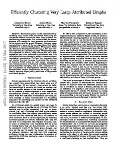
Metabolic pathway graph of valine, leucine and isoleucine degradation . . .
8
2.1
Pre-Post Labeling and Min-Post Labeling . . . . . . . . . . . . . . . . . . .
14
2.2
An example where SSPI size gets quadratic . . . . . . . . . . . . . . . . . .
16
2.3
GRIPP Index Table and Order Tree . . . . . . . . . . . . . . . . . . . . . .
18
2.4
Tree Cover Labeling . . . . . . . . . . . . . . . . . . . . . . . . . . . . . .
20
3.1
Min-Post Labeling . . . . . . . . . . . . . . . . . . . . . . . . . . . . . . .
37
3.2
Interval Labeling: Tree (a) and DAG: Single (b) & Multiple (c) . . . . . . .
39
3.3
Direct Exceptions: ci denote children and xi denote exceptions, for node u. .
46
4.1
Venn Diagram of Pairs wrt. Reachability . . . . . . . . . . . . . . . . . . .
52
5.1
Reachability Queries: (a) Positive (b) Deep Positive Distance . . . . . . . .
67
5.2
Effect of Increasing Number of Intervals on Small Graphs: (a) agrocyc, (b) amaze, (c) arxiv, (d) pubmed . . . . . . . . . . . . . . . . . . . . . . . . .
76
Effect of Increasing Number of Intervals on Large Graphs: (a) cit-patents, (b) citeseerx, (c) rand10m2x, (d) rand10m5x . . . . . . . . . . . . . . . . .
77
6.1
Sample input graph and its DAG . . . . . . . . . . . . . . . . . . . . . . .
80
6.2
DAGGER graph: i) Initial input graph Gi = (V i , E i ) is shown on the plane (solid black edges). The SCC components (V d ) are shown as double-circled nodes. Components consisting of single nodes are shown on the plane, whereas larger components are shown above the plane. DAG edges E d are not shown for clarity. Containment edges (E c ) are shown as black dashed arrows. ii) Insertion of the (dotted gray) edge (N, B) in Gi , merges five SCCs, namely {1, H, I, L, 3}, with 3 as the new representative. The thick gray dashed edges are the new containment edges. . . . . . . . . . . . . . .
82
6.3
Two valid initial labelings . . . . . . . . . . . . . . . . . . . . . . . . . . .
89
6.4
Merge Operation on the Index . . . . . . . . . . . . . . . . . . . . . . . . .
94
5.3
viii
Deletion of (gray dotted) edge (L, P ) from Gi . First, node L becomes a component by itself, and we remove the containment link (L, 3). Then H does the same. The call from B finds a path to the target node P via C, I, O, T, S therefore these nodes remain under 3 along with P . Note that we do not touch A and N since they will continue to remain under 3. Also the containment edges (B, 1) and (C, 1) are removed. Containment edges (B, 3) and (C, 3) are added when we lookup for their component, due to path compression within the union-find structure. However (A, 1) is remains unchanged. To reduce clutter, the DAG edges E d are not shown. . . . . . .
95
6.6
Split Operations on the Index . . . . . . . . . . . . . . . . . . . . . . . . .
99
6.7
Total time comparison on dynamic datasets . . . . . . . . . . . . . . . . . . 105
6.5
ix
ACKNOWLEDGMENT I am truly grateful to my advisor Professor Mohammed J. Zaki for his continuous support and guidance during my doctoral studies. This thesis would not have been possible without his direction and patience, not to mention his brilliant ideas on the research problems as well as his skill in expressing them in written form. His contributions have been unparalleled. I also would like to thank my M.S. advisor, Professor Mukkai Krishnamoorthy, for his support even after I completed my masters’s degree. I do not know how to express my profound gratitude to Vineet Chaoji, co-author of all the papers that made up this thesis. I have countless memories of our fruitful discussions that made this thesis possible, ranging from picking the thesis topic to interpreting the results of the latest experiments. He has always been there to listen and encourage me in any personal or academic issues, despite his super busy schedule and 12 hour time difference between India and United States. We could publish a book from our gmail chat records! The other two former members of our lab team - Mohammad Al Hasan and Saeed Salem- also deserve special thanks. I had the pleasure to share the lab with them in their final year; I only wish I could have joined that fun and industrious gang earlier. I would also like to thank the newer members: Medha Atre, Geng Li, and Pranay Anchuri. Having acknowledged the core research group, I now can thank to people who enabled me to enjoy my life in Troy. During the past six years, I have found many good friends in RPI, including—but not limited to— Ey¨uphan Bulut, Ali C¸ivril, C¸a˘gatay Bilgin, ¨ ¸ a˘glar, Bu˘gra Cas¸kurlu, Burak C¸avdaro˘glu and Aytekin Varg¨un. We have shared C¸agrı Ozc some unforgettable moments, such as winning the intramural soccer tournament. In the enlarged circle, I am indebted to many other people who supported me including Ali Can, ¨ Zafer Ak, Erol Akmercan, S¨uleyman Vural, Veysel Uc¸an, C¨uneyt G¨oz¨u and Asil Ozdo˘ gru. Last but most importantly, I want to express my deepest gratitude to my wife, Zeynep. She has always stood by me and given me unconditional support-despite my inability to balance my working hours between school and home. I greatly appreciate her patience. I am eternally grateful for her contribution to my life. I am also indebted and grateful to our family; for their continuous support and prayers.
x
ABSTRACT Answering reachability queries in graphs is an important problem. With the development of high-throughput data acquisition techniques and the advances in the areas of semantic web and social networks, we have abundance of enormous graph-structured data on which different queries are asked. One of the fundamental queries, a reachability query, asks whether there exists a path between any two given nodes. This can map to the question of whether one researcher has been influenced by another in a citation network; whether a protein inhibits or activates another one indirectly in a protein interaction network; whether a protein is broken down to a specific molecule in a metabolic pathway graphs; or whether a concept is subsumed by part of another in an ontology. Aside from these direct correspondences with real-life questions, they can constitute building blocks for complicated queries in various databases. Therefore, there is a crucial need for mechanisms that expedite querying in graph databases. Existing methods for reachability trade-off indexing time and space versus query time performance. However, the biggest limitation of existing methods is that they do not scale to very large real-world graphs. They are also vulnerable to increasing edge densities. Another limitation of the existing methods is that they barely, if at all, support dynamic updates. This is primarily due to the complex nature of the problem – a single edge addition or deletion can potentially affect the reachability of all pairs of nodes in the graph. Most of the previous work has focused on dynamically maintaining the transitive closure of a graph, which has the obvious O(n2 ) worst-case bound, where n is the number of nodes. Moreover, most of the static indexes cannot be directly generalized to the dynamic case. This is because these indexes trade-off the computationally intensive preprocessing/index construction stage to minimize the index size and querying time. For dynamic graphs, the efficiency of the update operations is another aspect which needs to be optimized. However, the costly index construction typically precludes fast updates. It is interesting to note that a simple approach consisting of depth-first search (DFS) can handle graph updates in O(1) time and queries in O(n + m) time, where m is the number of edges. For sparse graphs m = O(n) so that query time is O(n) for most large
xi
real-world graphs. Any dynamic index will be effective only if it can amortize the update costs over many reachability queries. In this thesis, we present two approaches for addressing the problems of scalable reachability indexing for both static and dynamic graphs. More specifically, we introduce two indexing schemes, namely GRAIL and DAGGER. GRAIL is a simple yet scalable reachability index that is based on the idea of randomized interval labeling, and that can effectively handle very large graphs. Based on an extensive set of experiments, we show that while more sophisticated methods work better on small graphs, GRAIL is the only index that can scale to millions of nodes and edges. GRAIL has linear indexing time and space, and the query time ranges from constant time to being linear in the graph order and size. Our second contribution is a scalable, light-weight reachability index for dynamic graphs called DAGGER which has linear (in the order of the graph) index size and index construction time, and reasonably fast update and query times. DAGGER is based on the idea of maintaining randomized interval labels for the nodes of the underlying acyclic graph (DAG) of the input graph. Therefore DAGGER yields an efficient algorithm for maintaining the strongly connected components of the evolving graph, which is of independent interest. We demonstrate the efficiency and effectiveness of DAGGER in large dynamic real-world networks such as Wikipedia graph and citation networks as well as synthetic dynamic graphs. In the future, we plan to improve the query time of DAGGER by maximizing the quality of the index while keeping the updates fast. We also plan to extend GRAIL and DAGGER for other variants of reachability problem such as constrained reachability and shortest path queries.
xii
1. INTRODUCTION Graph-based representation of data has become predominant with the emergence of largescale interlinked datasets, such as social networks, biological networks (e.g. protein interaction networks and metabolic pathways), call graphs, semantic RDF (resource description framework) graphs, and so on. For instance, Facebook has 750 million users with and average of 130 friends per user. This implies that the Facebook social graph has 750 million nodes, with approximately 49 billion edges. Similarly, RDF graphs with over a billion triples are quite common these days. Other examples include citation graphs, communication networks, and so on. The scale of these datasets has renewed interest in graph indexing and querying algorithms. Answering reachability queries in graphs is one such area. A reachability query asks if there exists a path from a source node to a target node in a directed graph. Answering graph reachability queries quickly has been the focus of research for over 20 years. Traditional applications for reachability include reasoning about inheritance in class hierarchies and testing concept subsumption in knowledge representation systems. However, interest in the reachability problem has revived in recent years with the advent of new applications which have very large graph-structured data that are queried for reachability excessively. The emerging area of Semantic Web is composed of RDF/OWL data which are indeed graphs with rich content, and there exist RDF data with millions of nodes and billions of edges. Reachability queries are often necessitated on these data to infer the relationships among the objects. In network biology, reachability play a role in querying protein-protein interaction networks, metabolic pathways and gene regulatory networks. In general, given the ubiquity of large graphs, there is a crucial need for highly scalable indexing schemes for reachability queries. For these graph databases where the underlying graph is static, a reachability index is constructed once and it is never updated. On the other hand, most of the real world networks undergo update operations. These updates include addition and deletion of edges or nodes. Citation networks get updated as new papers are added. An update corresponds to a node addition in the graph along with new outgoing edges to their references. In social network such as Twitter
1
2
and Facebook, it is not surprising to see a dynamically changing graph structure as new connections emerge or existing ones disappear. Communication networks also update the routing information based on congestion along certain paths or the addition of new lines. Web graph undergoes frequent updates with new links between pages. Wikipedia is a representative example wherein links are added as new content pages are generated, and deleted as corrections are made to the content pages. In such a dynamic setting, a reachability index has to adapt itself to the changes on the indexed graph. Given the scale of the above graphs, recomputing the entire index structure for every update is computationally prohibitive. Moreover, for online systems that receive a steady volume of queries, recomputing the index would result in system down-time during index updation. As a result, a reachability index that can accommodate dynamic updates is desired.
1.1 Problem Formulation and Notations A database graph is an unlabeled directed graph G = (V, E) where V is the set of vertices and E is the set of edges. Note that in an undirected graph the problem is trivial to solve, one just has to find the connected components to answer reachability queries. G has |V | = n nodes and |E| = m edges. Definition 1 (Reachability) Given two vertices u and v in directed graph G, where u, v ∈
V , if there exists a path p from the source node u to the target node v, then we say u can
reach v, notated as u
v. If u cannot reach v, we denote it as u 6
u and v, the reachability query asks if u
v and it is notated as u
v. Given two vertices ?
v.
It is worth noting at the outset that the problem of reachability on directed graphs can be reduced to reachability on directed acyclic graphs (DAGs). Given a directed graph G, we can obtain an equivalent DAG, G′ (called the condensation graph of G), in which each node represents a strongly connected component of the original graph, and each edge represents the fact whether one component can reach another. To answer whether node u can reach v in G, we simply look up their corresponding strongly connected components, Su and Sv , respectively, which are the nodes in G′ . If Su = Sv , then by definition u and reach v (and vice-versa). If Su 6= Sv , then we pose the question whether Su can reach Sv
in G′ . Thus all reachability queries on the original graph can be answered on the DAG.
3
Figure 1.1 shows an example directed graph and the corresponding DAG obtained by coalescing the strongly connected components that are marked in dashed circles. In that graph N
?
P is true since they are in the same component. The query of G
original graph is equivalent to the query of 2
?
?
P in the
8 in the corresponding DAG. Henceforth,
you can assume that all input graphs have been transformed into their corresponding DAGs unless otherwise stated. R
A
D
E 0
B
C
H
I
F
G 1
K
N
3
L
T
S
O
2
J
M
4
5
7
6
P 8
(a) A Directed Graph
9
(b) Corresponding DAG
Figure 1.1: Coalescing strongly connected components Definition 2 (Reachability Indexing Mechanism) A reachability indexing mechanism R = (L, Q) is composed of two functions. A reachability labeler L : G → L is a function
L(G) = L that assigns a labeling L for each graph G. A labeling L = {L1 , L2 , . . . , Ln }
is composed of the labels of each node which is an array of bits. A query resolver Q is
a function that provides a boolean value given a labeling and two query nodes. It is said to be comparator if Q requires just the labels of the two query nodes, (i.e. Q(Lu , Lv ) =
{true, f alse}). A query resolver is called searcher if it also requires the labels of the
non-query nodes or the graph structure, (i.e. Q(u, v, L, G) = {true, f alse}).
The quality of a reachability indexing mechanism R is measured based on the following objectives depending on the requirements of the application. Objective 1 Query Time: The time taken to answer a reachability query using Q.
4 Objective 2 Index Size: The total size of the labeling L produced by L. Objective 3 Construction Time: The time taken to produce a labeling L using L. Query time is the most important measure most of the time as the goal of indexing is to provide fast querying. Nevertheless an indexing should keep a balance of these objectives depending on the graph structure and application type. Most of the existing methods focus on optimizing query time and index size and ignore construction time as long as it has polynomial time complexity. The main reason is that labeling is a one time activity and a slightly longer time can be tolerated. However the construction time becomes important when the graph is very large or when it has to be updated periodically if the graph is evolving. A scalable indexing scheme is possible only when it has linear construction time. The first contribution of this thesis is such a scalable reachability index for static graphs called GRAIL. It also constitutes the skeleton for the second contribution of this thesis; DAGGER, a scalable reachability index for dynamic graphs. Objective 4 Update Time: The time taken to update the labeling L when the graph G undergoes an update operation. The update time is a little vague as it depends on the granularity of the supported update operations. An update can be an insertion of a new subgraph to the existing graph as well as a deletion of a single edge. Some existing studies define it as bulk update which involves many edges and nodes, while others consider only single edge/node insertions and deletions. In this thesis, we further divide update time into four types according to the type of the update operation as different operations can have quite different computational complexities. Objective 5 Simulation Time: The total time taken to answer all queries using L while updating L given a sequence of intermixed query and update operations. Dynamic indexes are difficult to evaluate and compare with each other since there are many objectives to consider. A dynamic index can be really fast at answering queries however it is not very useful if it has to modify the labels of many nodes in the case of very common update. However for some update operations that occurs very rare, an inferior
5
update time can be tolerated. To be able to make a comparison between the methods, we generate benchmark sequences of intermixed query and update operations inspired from real-world scenarios. Full Transitive Closure
O(nm) O(1)
Construction Time Query Time
2
O(n )
Index Size
DFS/BFS
O(1) O(n + m) O(1)
Figure 1.2: Tradeoff between Query Time and Index Size There are two basic approaches to answer the reachability queries which lie at the two extremes of the index design space, as illustrated in Figure 1.2. Given a DAG G, with n vertices and m edges, one extreme (shown on left) is to precompute and store the full transitive closure; this allows one to answer reachability queries in constant time by a single lookup, but it unfortunately requires a quadratic space index, making it practically unfeasible for large graphs. In formal terms, this is a comparator indexing in which the labeler assigns an array of bits of size n for each node and the query resolver just checks a specific bit of the label of the query node. On the other extreme (shown on right), one can use a depth-first (DFS) or breadth-first (BFS) traversal of the graph starting from node u, until either the target, v, is reached or it is determined that no such path exists. This approach requires no index, but requires O(n + m) time for each query, which is unacceptable for large graphs. In formal terms, this can be counted as a searcher indexing in which labeler does nothing and the query resolver needs to find a path in the graph to determine the reachability. Existing approaches to graph reachability indexing lie inbetween these two extremes. A thorough survey of the existing algorithms is given in chapter 2.
1.2 Motivating Applications There may be a need for reachability labelers in any application where the underlying data is a directed graph. Due to the expressive power of graphs, it is not very uncommon to come across such applications in the domains of bioinformatics, semantic
6
web, compilers, social networks, geographical information systems, ontologies etc. We give below some examples where an index structure for reachability queries is a necessity. • Semantic Query Engines: The vision of the semantic web is to allow machines to understand the meaning of the information on the world wide web [1]. The data stores and interchange formats used include RDF and XML. The main structure of XML documents are trees but with the use of ID/IDREF links it is possible to represent graphs. On the other hand everything is relationships in RDF documents and an RDF document naturally defines a graph. XQuery and SPARQL are the query languages for XML and RDF respectively. SPARQL lets the user define graph patterns in SQL-like syntax that are to be searched in an RDF store. With SPARQL 1.1 it will be possible to search patterns that includes paths of arbitrary lengths via property paths [2]. For example the following SPARQL query asks all the researchers named Joe Example who might be influenced by the paper titled Sample Paper in a citation database. SELECT ?name WHERE { ?x foaf:name ?name . ?y citation:title ?title . ?y citation:author ?x . ?x citation:cites+/citation:title ?pname . FILTER regex(?name, "Joe Example") FILTER regex(?pname, "Sample Paper") } Figure 1.3: A SPARQL query that uses property paths A query engine can list the result following two different strategies. One is traversing the whole subgraph which cites the paper Sample Paper directly or indirectly and checking if Joe Example is the author for each paper. The other strategy is going over the papers of Joe Example and checking whether they are reachable via citation links. Considering that a typical paper has tens of citations, the second strategy seems inevitable if an efficient reachability index exists. With SPARQL 1.1 the necessity for reachability indexes in RDF stores will become more apparent. • Concept Subsumption in Ontologies: In knowledge representation systems, on-
7
tologies define a set of concepts and their properties and relationships between each other within a domain. They are used to describe a domain or to reason about the entities within a domain. In semantic web, inference engines generate all the possible conclusions and store the resulting triples in the datastore as well. For instance, if a class A is a subclass of B which is a sublass of C, it infers that A is a sublass of C and stores that fact in the database. This method is also used in the Gene Ontology project which defines the concepts on genes. The ontology basically represents a directed acyclic graph of terms however the Gene Ontology [3] database also includes the inferred relationships to speed up querying [4]. This is equivalent to keeping the transitive closure of the graph all the time in the database and it is not scalable for very large graphs. An alternate strategy is to avoid inference computation at least for transitive rules such as rdfs:subPropertyOf and rdfs:subClassOf [5]. In this case the inference engine should infer these relations on-demand using a reachability labeling mechanism. One of the test cases of our experimental evaluation in chapter 5 is composed of the terms of the Gene Ontology and the gene products from Uniprot [6] annotations database. The overall data has more than 7 million nodes and 56 million connections. • Biological Networks: With the advance of high-throughput data acqusition technologies, biologists have amassed a large amount of heteregenous graph data such as metabolic pathway databases, gene regulatory networks, signal transduction networks, etc. In these datasets nodes represent entities such as proteins, genes, compounds and edges represent how they interact. A query of whether a gene A regulates gene B directly or indirectly in a gene regulatory network maps to a reachability query. For example in figure 1.4, a metabolic pathway graph of the amino acids valine, leucine and isoleucine degradation obtained from KEGG [7] pathway database is shown. Valine, leucine and isoleucine are essential amino acids for humans and they have to be obtained from the diet as they can not be produced by the body. The fact that leucine breaks down to acetyl-coa classifies leucine as ketogenic whereas valine is not ketogenic since it does not break down to acetyl-coa [8]. These are indeed just reachability queries from the given amino-acids to the molecule acetyl-coa.
8
Figure 1.4: Metabolic pathway graph of valine, leucine and isoleucine degradation
9
1.3 Outline As shown above, reachability queries in large directed graphs is an important task with wide ranging set of applications. This thesis presents efficient and scalable methods for reachability indexing and querying in massive graph databases. Chapter 2 provides comprehensive survey of the existing indexing mechanisms with specific emphasis on interval-labeling methods. Chapter 3 focuses on our first contribution, GRAIL [9, 10], a scalable randomized interval-labeling based reachability indexing mechanism. GRAIL forms the backbone of the thesis as our dynamic index DAGGER is also built on it. In chapter 4 we present optimizations for GRAIL which greatly improves the query performance in static graphs. Chapter 5 presents an comprehensive experimental analysis of GRAIL, evaluating the impact of all the optimizations and parameter selections. In chapter 6, we propose DAGGER, a scalable index for reachability queries in large dynamic graphs. Finally we conclude in chapter 7 with a brief summary of results and possible future research directions in reachability indexing.
2. RELATED WORK Existing approaches for graph reachability combine aspects of indexing and pure search, trading off index space for querying time. Major approaches include interval labeling, compressed transitive closure, and 2HOP indexing [11, 12, 13, 14, 15, 16, 17, 18, 19, 20, 21, 22, 23], which are discussed below, and summarized in Table 2.1.
Opt. Tree Cover [11] GRIPP [12] Dual Labeling [13] PathTree [14] 2HOP [18] HOPI [19]
Construction Time O(nm) O(m + n) O(n + m + t3 ) O(mk) or O(mn) O(n4 ) O(n3 )
Query Time O(n) O(m − n) O(1) 2 O(log √ k) O(√m) O( m)
Index Size O(n2 ) O(m + n) O(n + t2 ) O(nk) √ O(n√m) O(n m)
Table 2.1: Comparison of Approaches: n denotes number of vertices; m, number of edges; t = O(m − n), number of non-tree edges; k number of paths/chains; and d number of intervals. Optimal Tree Cover [11] is the first known variant of interval labeling for DAGs. The approach first creates interval labels for a spanning tree of the DAG. This is not enough to correctly answer reachability queries, as mentioned above. To guarantee correctness, the method processes nodes in reverse topological order for each non-tree edge (i.e., an edge that is not part of the spanning tree) between u and v, with u inheriting all the intervals associated with node v. Thus u is guaranteed to contain all of its children’s intervals. Testing reachability is equivalent to deciding whether the interval list of the source node subsumes the first interval of the target node. The construction complexity of this method is the same as a full transitive closure. GRIPP [12] is another variant of interval labeling. Instead of inflating the index size for the non-tree edges as in [11], reachability testing is done via multiple containment queries. Given nodes u and v, if Lv is not contained in Lu , the non-tree edges (x, y), such that x is a descendant of u, are fetched, and recursively a new query (y, v) is issued for every y, until either v is reachable from a y node or if all non-tree edges are exhausted. If one of the y nodes can reach v then u can reach v. Since there are m − n non-tree edges, the query time complexity is O(m − n).
10
11
Dual labeling [13] also uses interval labeling but it processes non-tree edges in a different way. Their main observation is that if there exists a single non-tree edge (x, y) in the path from u to v, it must be true that Lu contains x and Ly contains v. Based on this, a non-tree edge e = (x, y) is connected to another non-tree edge e′ = (x′ , y ′ ) if and only if Ly contains Lx′ . After labeling the selected tree, dual labeling computes the transitive closure of non-tree edges so that the entry for the edge pair (e = (x, y), e′ = (x′ , y ′ )) being 1 implies that all nodes u, whose interval contains x, can reach all nodes v whose interval is contained by Ly′ . Therefore for each query they scan relevant edge pairs to find out the reachability. With further optimizations, they reduce the query time to O(1), however their index size is O(n + t2 ), and construction time is O(n + m + t3 ) where t = O(m − n) denotes the number of non-tree edges. A chain decomposition approach was proposed in [15] to compress the transitive closure. The graph is split into node-disjoint chains. A node u can reach to node v if they exist in the same chain, and u precedes v. Each node also keeps the highest node that it can reach in every other chain. Thus the space requirement is O(kn) where k is the number of chains. Such a chain decomposition is computed in O(n3 ) time. This bound was improved in [16], where they proposed a decomposition which can be computed √ in O(n2 + kn k) time. Recently, [24] further improved this scheme by using general spanning trees in which each edge corresponds to a path in the original graph. [17] solves a variant of the reachability problem where the input is assumed to be a collection of non-disjoint paths instead of a graph. PathTree [14] is the generalization of the tree cover approach. It extracts the disjoint paths of a DAG, then creates a tree of paths on which a variant of interval labeling is applied. That labeling captures most of the transitive information and the rest of the closure is computed in an efficient way. PathTree has very fast querying and construction times, but its index size might get very large on dense graphs (k denotes the number of paths in the decomposition). In a recent paper by the same authors, they proposed 3HOP [25] which addresses the issue of large index size. Although 3HOP has a reduced index size, the construction and query times degraded significantly. The other major class of methods is based on 2HOP Indexing [18, 19, 20, 21, 22, 23], where each node determines a set of intermediate nodes it can reach, and a set of
12 intermediate nodes which can reach it. The query between u and v returns success if the intersection of the successor set of u and predecessor set of v is not empty. 2HOP was first proposed in [18], where they also showed that computing the minimum 2HOP cover is NP-Hard, and gave an O(log m)-approximation algorithm based on a greedy algorithm set-cover problem. Its quartic construction time was improved in [21] by using a geometric approach which produces slightly larger 2HOP cover than obtained in [18]. A divide-and-conquer strategy to 2HOP indexing was proposed in [19, 20]. HOPI [19] partitions the graph into k subgraphs, computes the 2HOP indexing within each subgraph and finally merges their 2HOP covers by processing the cross-edges between subgraphs. [20], by the same authors, improved the merge phase by changing the way in which cross-edges between subgraphs are processed. [22] partition the graph in a top-down hierarchical manner, instead of a flat partitioning into k subgraphs. The graph is partitioned into two subgraphs repeatedly, and then their 2HOP covers are merged more efficiently than in [20]. Their approach outperforms existing 2HOP approaches in large and dense datasets. The HLSS [23] method proposes a hybrid of 2HOP and Interval Labeling. They first label a spanning tree of the graph with interval labeling and extract a remainder graph whose transitive closure is yet to be computed. In the transitive closure of the remainder graph, densest sub-matrices are found and indexed with 2HOP indexing. The problem of finding densest sub-matrices is NP-hard and they proposed a 2-approximation algorithm for it. Despite the overwhelming interest in static transitive closure, not much attention has been paid to practical algorithms for the dynamic case, though several theoretical studies exist [26, 27, 28]. Practical works on dynamic transitive closure [29, 30] and dynamic 2HOP indexing [31, 32] have only recently been proposed.
2.1 Interval Labeling Approaches While there is not yet a single best indexing scheme for DAGs, the reachability problem on trees can be solved effectively by interval labeling [33], which takes linear time and space for constructing the index, and provides constant time querying. Given a tree/forest T = (V, E) that has |V | = n edges and |E| = m edges, interval labeling
13 assigns each node u a label Lu = [su , eu ] which represents an interval starting at su and ending at eu . A desired labeling has to satisfy the condition that Lu subsumes Lv if and only if u reaches v. Therefore a reachability query of u
?
v can be answered just by
comparing the corresponding intervals. Namely u reaches v if and only if su ≤ sv and
ev ≥ ev .
Pre-Post Labeling, first interval labeling scheme for trees, was proposed by Dietz et al. [33]. Many of the following studies exploited that scheme for directed acyclic graphs [33, 12, 34, 14]. Min-Post Labeling [11, 9] provides an equivalent labeling for trees but it differs in directed acyclic graphs. Pre-Post Labeling assigns Lu = [su , eu ] to each node u where su and eu are obtained via a depth-first traversal from the roots. A counter is incremented both when DFS enters a node and leaves a node. su and eu are the values of that counter at the entrance and the termination of the node u, respectively. Min-Post Labeling assigns Lu = [su , eu ] to each node u where eu = post(u) is the post-order value of the node u and su = min{sx |x ∈ children(u)} that is also equal to min{ex |x ∈ descendants(u)}. Therefore, su denotes the lowest rank for any node x in
the subtree rooted at u (i.e., including u)
In both of the methods, the containment between intervals is equivalent to reachability relationship. In Pre-Post Labeling, su is less than sx and eu is greater than ex for any descendant x of u since a depth-first traversal enters a node u before all of its descendants and leaves after having visited all of its descendants. In Min-Post Labeling, su is always smaller than or equal to its descendants by definition and eu inequality holds as similar to pre-post labeling. Figure 2.1(a)(b) shows these labelings on a tree, assuming that the children are ordered from left to right. It is easy to see that reachability can be answered by interval containment in both labelings even though the labels are quite different. For example in Pre-Post Labeling, 1 26
9, since L9 = [7, 8] ⊂ [2, 13] = L1 , but
7, since L7 = [4, 9] 6⊆ [14, 19] = L2 whereas in Min-Post Labeling 1
L9 = [2, 2] ⊂ [1, 6] = L1 , but 2 6
9, since
7, since L7 = [1, 3] 6⊆ [7, 9] = L2
In Figure 2.1(c)(d) pre-post and min-post labeling is applied to a directed acyclic graph which is obtained by the addition of the dashed edges to the tree. The labeling of pre-post labeling does not change at all because the dashed edges are never followed since
14
0 [1,20]
1 [2,13]
0 [1,10]
2 [14,19]
1 [1,6]
3 [3,10] 4 [11,12] 5 [15,18]
3 [1,4]
7 [4,9]
6 [16,17]
8 [5,6]
0 [1,10]
1 [1,6]
3 [3,10] 4 [11,12] 5 [15,18]
3 [1,4]
7 [4,9]
8 [5,6]
9 [2,2]
(b) Min-Post Labeling
2 [14,19]
6 [16,17]
5 [7,8]
7 [1,3]
8 [1,1]
0 [1,20]
1 [2,13]
4 [5,5]
6 [7,7]
9 [7,8]
(a) Pre-Post Labeling
2 [7,9]
9 [7,8]
(c) Pre-Post Labeling on DAG
2 [1,9]
4 [1,5]
5 [1,8]
7 [1,3]
6 [1,7]
8 [1,1]
9 [2,2]
(d) Min-Post Labeling on DAG
Figure 2.1: Pre-Post Labeling and Min-Post Labeling their end nodes are already visited. However, in this case labeling misses some of the reachable pairs. For example, 2
7 but L2 = [14, 19] 6⊆ [4, 9] = L7 . On the other hand,
min-post labeling captures all reachable pairs. For example L2 = [1, 9] ⊆ [1, 3] = L7 . However it falsely categorizes some pairs as reachable. e.g. L5 = [1, 8] ⊆ [1, 5] = L4 but
56
4. Namely, pre-post labeling has no false-positives whereas min-post labeling has
no false-negatives. The existing interval labeling approaches extend pre-post labeling or min-post labeling for directed graphs. We investigate these approaches in two categories. In the first group, a search strategy is used based on the labels of the nodes which may require many label comparisons. In the second group, the reachability between the target and source is
15
determined just by comparing the corresponding labels. 2.1.1
Online Search Methods In this section, we introduce the approaches that might need to compare the labels
of several nodes to answer a reachability query. Assigning intervals to the nodes beforehand based on one of the labelings from Figure 2.1 is the common first step of these approaches. A single label comparison between the target and source nodes is not sufficient to conclude a result so these methods perform a search on the graph. However the labelings speed up the search process either by providing hop points or by pruning some branches of the search tree. Their worst case query time is linear with respect to the graph size. 2.1.1.1
Tree + SSPI
Chen et al. propose an interval labeling approach in [34] which is supplemented by a predecessor index to ease the traversal in the graph. In the first stage of the algorithm a spanning tree T of the graph G is selected and encoded by pre-post interval labeling. The set of edges in T is called ET and the remaining set of edges is called ER . In our running example, the labeling is as in Figure 2.1(c) and the dashed edges constitute ER . In addition to the interval labeling, a predecessor list,P L(u), is kept for each node u. There are two types of predecessors in this list; surrogate predecessors and immediate surplus predecessors. Any path p in a DAG G, is a mix of tree edges and non-tree edges. If a path p is composed of only tree edges, the reachability relation is captured by interval labeling. For every path in the form of er (et )∗ that ends at node u, a predecessor is added to the list of u. Assume the edge er connects the node x to the node y. If y equals to u, then x is added to P L(u) as an immediate surplus predecessor. Otherwise y is added as a surrogate predecessor of the node u. In our example graph in Figure 2.1(c), nodes 2, 4, and 6 are the immediate surplus predecessors of the nodes 3, 8 and again 8 respectively because the edges (2, 4), (4, 8) and (6, 8) are the non-tree edges of the graph. Furthermore node 3 is a surrogate predecessor for the nodes 7, 8 and 9 as there can be found paths that start with the non-tree edge (2, 3) and followed by tree edges ending at the nodes 7, 8 and 9.
16
SSPI Construction: The SSPI is constructed in linear time proportion to the size of G via performing a tree traversal in a top-down fashion. For each node u, immediate surplus predeccesors are trivial. (the non-tree edges ending at node u.) The construction algorithm depicted in [34] is as follows: • At each node u in the spanning tree traversal – Collect immediate surplus predeccesors of u into P L(u) – Inherit P L(w) (i.e. the predecessor list of w) where w is the parent of u in the spanning tree The predeccesor lists constructed in this way are not conformant with the definition of SSPI. In our running example, node 3 gets 2 as immediate surplus predecessor and nodes 7, 8 and 9 inherits 2. Indeed, node 3 should be the surrogate predecessor of the nodes 7, 8 and 9. In the paper, it is also claimed that the total number of predeccesors stored in SSPI is bounded by O(m) which we disprove by a counter example in Figure 2.2. As seen in the figure, X,Y , Z and T are the immediate surplus predeccesors for C,D,E and F respectively. Furthermore, D inherits X from C. E inherits {X, Y } from D
and finally F inherits {X, Y, Z} from E. One can find such graphs where SSPI size is
quadratic even though the number of edges m = O(n).
A [1,20]
[18,19] X
[15,16] Y
[12,13] Z
[9,10] T
B [2,17]
C [3,14]
D [4,11]
E [5,8]
w C D E F
F [6,7]
(a) Interval Labeling
P L(w) X X, Y X, Y, Z X, Y, Z, T
Figure 2.2: An example where SSPI size gets quadratic Querying: If there is a tree-path between the source node u and the target node v, it can easily be checked from their interval labeling. If Lu contains Lv , that concludes u reaches v. Otherwise, the reachability between u and the nodes in the P L(v) has to be checked recursively. If any of the recursive calls return success, then we again conclude that u reaches v. If all of the recursive calls fails to find a path, the pair is not connected. For example, in our toy graph in Figure 2.1(c) the query 2
?
9 is performed. L2 does not
17
contain L9 , so the query will continue with 2
?
2 (because 2 ∈ P L(9)). Since that query
is true, we conclude that 2 can reach to 9. The running time of the algorithm is O(n) since there is no need to query a pair more than once. Figure 2.2 is an example to the class of graphs where a reachability query takes O(n) time (e.g., between X and F ). 2.1.1.2
GRIPP
In [12] Trißl et al. proposed GRIPP, another variant of pre-post labeling. In GRIPP, each node is assigned as many intervals as it has incoming edges. Basically, the depth-first traversal is modified so that when the traversal encounters with an already visited node (i.e. via a non-tree edge), it assigns another interval without traversing the children of that node. A node u with k incoming edges are visited k times. In the first visitation it gets the pre-order value and proceeds the traversal with its children and assigns the post-order value at the end. However for the remaining k − 1 visitations (via a non-tree edge, i.e., dashed edges in our graphs), u is assigned a unit interval and its children are not traversed.
These intervals are kept in a table called index table, IN D(G). For instance, in our running example in Figure 2.1(c) the dashed edges are again the non-tree edges. The index table of that graph is shown in Table 2.1.1.2. The first visited non-tree edge is (4, 8) and that edge adds the interval [12, 13] to node 8. Similarly, once the non-tree edge (2, 3) is processed, node 3 is assigned its second interval which is [17, 18]. Note that its children are not revisited after that point. The GRIPP index structure can also be viewed as a rooted tree where each edge of the original graph G (equivalently every instance in IN D(G)) corresponds to a node in that tree. That tree is called Order Tree, O(G). Every non-tree instance of IN D(G) is a leaf node in O(G) because their children are not traversed. Tree instances can be leaf nodes or inner nodes. An Order Tree can be plotted in pre-post order plane as shown in Figure 2.3. The non-tree instances are depicted as diamond nodes in the example order tree. Querying : Reachable Instance Set of a node u in graph G, RIS(u), is the set of instances that are reachable from u in O(G). RIS(u) can be retrieved by querying the instances v in IN D(G), which has the property s(u) ≤ s(v) ≤ e(u). For the query s
?
t, GRIPP first checks whether an instance of t exists in RIS(s). If not, all the
18 node 0 1 3 7 8 9 4 8 2 3 5 6 8
pre 1 2 3 4 5 7 11 12 16 17 19 20 21
post 26 15 10 9 6 8 14 13 25 18 24 23 22
type tree tree tree tree tree tree tree non-tree tree non-tree tree tree non-tree
Table 2.2: GRIPP Index Table
[1,26] 0 25
2 [16,25] 5 [19,24] 6 [20,23] 8
[21,22]
20 3 15
[17,18]
[2,15] 1 4 [11,14] 8
10
[12,13]
[3,10] 3 [4,9] 7
9 [7,8]
8 [5,6] 5 0
5
10
15
20
25
Figure 2.3: GRIPP Index Table and Order Tree non-tree instances in RIS(v) is captured and the querying proceeds recursively from the tree instances of the captured non-tree instances. For example, for the 2
?
9 query in
Figure 2.3, node 9 does not exist in RIS(2). Therefore the non-tree instances (diamond
19 nodes) of 3 and 8 is captured. The traversal terminates with a positive result since 9 ∈
RIS(3). To conclude with a negative result, the traversal has to exhaust all of the captured
non-tree instances. In IN D(G) there exists m − n non-tree instances, therefore a query
might require to capture m − n non-tree instances to conclude with unreachability in the worst case. The authors also study how to reduce the query time. There are m − n non-tree
instances but they correspond to at most n tree instances. Therefore just by keeping a list of used tree instances (aka hop nodes) most of the traversal is pruned. It is also possible to skip hop nodes that are subsumed by an already used hop node. Thus the processing order of the captured non-tree instances plays an important role on the querying performance. Trißl and Leser also observe that the ordering of the nodes used during the construction of the GRIPP index is important. To be able to reduce the number of hops that is required by a query, the nodes that have large reachable sets should be visited as early as possible. Consider the case where a node w with a very large reachable instance set is visited late in the index construction. In that scenario, w will have a narrow interval which is mostly composed of non-tree instances which in turn would cause many hops during querying. The authors conclude that finding optimal traversal is NP-Complete and impractical. They propose a few heuristics such as ordering nodes by their indegrees and starting the traversal from an estimated giant strongly connected component. 2.1.2
Label Comparison Methods In this section we present the methods that are based on interval labeling and that
can answer queries just by comparing the labels of the nodes in question. This does not directly imply constant query time as the label sizes per node can get very large. 2.1.2.1
Optimum Tree Cover
The first non-trivial solution to the reachability problem in the database community is proposed by Agrawal et al. [11] in 1989. The main idea of the proposed method, Tree Cover, is to cover the full transitive closure via intervals obtained by min-post labeling of a spanning tree of the graph. In the first step of the algorithm a spanning tree is extracted and labeled. Figure 2.4(a) shows that labeling on our example graph. As opposed to the
20
labeling in Figure 2.1(c), that labeling does not consider non-tree edges in its first step at all. Similar to other methods, Lv ⊆ Lu only when u
v only via tree edges.
To be able to cover the non-tree edges (u′ , v ′ ), the node u′ inherits the intervals of
the node v ′ . That way u′ gains reachability to all the nodes reachable from v ′ . Nodes inherit these additional intervals in reverse topological order so that by the time of u′ is inheriting the interval of v ′ , v ′ should have captured its full reachability. In Figure 2.4(b), firstly node 6 gets the interval [1, 1] due to the non-tree edge (6, 8). Afterwards node 4 inherits [1, 1] too. Node 5 also inherits [1, 1] since the label of 6 is updated. Finally node 2 gets [1, 4] due to the edge (2, 3). If there was another edge from 2 to 4, node 2 would inherit node 4’s intervals which are [5, 5] and [1, 1]. Therefore the new value of 2 would become [7, 9][1, 4][5, 5][1, 1]. However the intervals subsumed by others can be discarded and adjacent intervals can be merged to compress the indexing and to reduce the query time. In that case the label of 2 can be reduced to [7, 9][1, 5]. At the completion of the labeling each node u is assigned a set of intervals Lu = {Lu1 = [s(u1 ), e(u1 )] , . . . , Luk =
[s(uk ), e(uk )]} where Lu1 is the interval assigned by the initial labeling of the spanning tree. After the labeling is completed, a query u an interval in Lu which contains Lv1 . Thus u
?
?
v is true if and only if there exists
v can be answered in O(log k) if u has
k intervals by performing a binary search. In the worst case each node might get linear number of intervals which makes the query time O(log k). The worst case seem to occur when a large number of nodes have a large set of common children. (e.g., dense bipartite graphs) The storage requirement is quadratic in the worst case because of the same reason. Given a graph, one can use many different spanning trees in the first step of the labeling. However not all trees provide equally good labelings in terms of the label size and the query time. In [11] an algorithm for selecting the spanning tree which gives the minimum labeling size is given. That tree is called optimum tree and the labeling obtained by it is called Optimum Tree Cover. The optimum tree selection algorithm minimizes the total number of intervals. It relies on the fact that if a node u and node w are the immediate predeccesors of the node v, and the edge (u, v) is selected in the spanning tree, then all the predeccesors of w that are not predeccesors of u will have to inherit the intervals of v. The algorithm selects a parent for each node by comparing the predeccesor lists of
21
0 [1,10]
1 [1,6]
0 [1,10]
2 [7,9]
1 [1,6]
3 [1,4] 4 [5,5] 5 [7,8]
3 [1,4]
6 [7,7]
7 [1,3]
6
4
[5, 5] [1, 1]
[7, 7] [1, 1]
8 [1,1] 9 [2,2]
8 [1,1]
(a) Min-Post Labeling on the Spanning Tree
0 [1,100]
2
[7, 9] [1, 4]
1
[1, 60] [61, 70]
5
[7, 8] [1, 1]
3
[1, 40] [41, 50] [61, 80] 4 5 [1, 10] [1, 10] [61, 70]
7 [1,3]
6
[61, 70] [1, 10]
9 [2,2]
10 [61,65]
(b) Tree Cover Labeling
2
[71, 90] [1, 40]
7 [1,30]
8 [1,10]
9 [11,20]
(c) Dynamic Operations on Tree Cover
Figure 2.4: Tree Cover Labeling its immediate predeccesors. The proposed algorithm runs in O(nm) time. Therefore the Tree Cover Labeling construction time is O(nm). The authors also considered the update operations to handle dynamic graphs. In order to accept new nodes, the initial labeling assigns non-contigous numbers. For example Figure 2.4(c) shows the case when the postorder counter is incremented by 10. There are 4 cases to consider. • New Node Addition: The interval of the parent is divided into two and first part is assigned to the new node (e.g. the red node and edge in Figure 2.4(c)). • Non-Tree Edge Addition: The labels of the child are propagated to predeccesors unless they already subsume it. For example in Figure 2.4(c), the addition of the blue edge causes node 3 to inherit [61, 70] as it already subsumes [1, 10]. Then node 1 inherits [61, 70] from node 3. However node 2 does not inherit as it already covers that interval and propagation stops. • Non-Tree Edge Deletion: The spanning tree is not changed. The non-tree labels of all nodes are recomputed by a scan over the nodes in reverse topological order. The time complexity is O(m). • Tree Edge Deletion: If a tree edge (u, v) is removed, node v becomes a new root in the spanning tree (i.e forest in this case). All the tree intervals of the nodes at the
22 subtree of v is shifted so that they are larger than the current largest value. Their non-tree intervals do not change. And the nodes in the rest of graph updates their non-tree intervals referring to the shifted intervals. For example if the edge (3, 7) is to be removed, the intervals of nodes 7, 8 and 9 will become [101, 130], [101, 110] and [111, 120] respectively. In the rest of the graph all nodes 0 to 6 have to update their intervals referring to [1, 10] to [101, 110]. 2.1.2.2
Dual Labeling
Dual Labeling [13] is a variant of interval labeling which efficiently compresses the residual transitive closure after labeling of a spanning tree of the graph. Similar to TreeCover, the first step of labeling a spanning tree captures the nodes that are reachable just via tree edges. The authors use Pre-Max Labeling to encode the selected tree. It assigns the label Lu = [s(u), e(u)] to node u, where s(u) is the pre-order of that node and e(u) is the maximum of s(v) + 1 where v is a node in the subtree rooted at u. However this labeling is equivalent to Tree Cover’s min-post labeling in terms of reachability coverage. Dual Labeling differs from [11] in the way it handles non-tree edges. The query u
?
v can be answered positively if the predicate s(v) ∈ Lu is true. It
means that u can reach v via tree edges. If there is just one link
1
in the path between
u and v, then there must exist a link (u′ , v ′ ) such that s(u′ ) ∈ Lu and s(v) ∈ Lv′ . A link (u′ , v ′ ) is connected to (x′ , y ′ ) if s(x′ ) ∈ Lv′ . All pairs of links of that kind is put
into a table called link table. Therefore the reachability with two links between u and v
is positive if there exists two links l1 = (u′ , v ′ ) and l2 = (x′ , y ′ ) such that s(u′ ) ∈ Lu , s(v) ∈ Ly′ and l1 is connected to l2 in the link table. One can answer queries that contain
any number of intermediate links by using the same scheme, if the transitive closure of the link table (a.k.a transitive link table) is computed and used instead of the link table. Following the above discussion, the overall query process is as follows. First it is checked whether the query nodes are connected via tree edges in O(1) time. If not, the transitive link table is scanned for the existence of a connected link pair l1 and l2 such that u reaches l1 via tree edges and l2 reaches v via tree edges. Since the size of the transitive link table is O(t2 ), the overall process takes O(t2 ) time. 1
In [13], non-tree edges are called “links”. We use the same terminology in this section.
23
To avoid scanning the transitive link table, Wang et al. compute transitive link counts. The informal definition of N (x, y) is the number of links l′ = (u′ , v ′ ) such that x is smaller than the preorder of u′ (i.e. s(u′ )) that can reach to the node whose preorder value is y. (i.e. y ∈ L′v ) Once these values are computed for each pair, one can find out
if there is any path between u and v having at least one link by checking the predicate N (s(u), s(v)) − N (e(u), s(v))) > 0. It basically checks the existence of a link that starts in the range [s(u), e(u)] that reaches to node v. Thus, the query time is reduced to O(1)
with the cost of increasing the index size to O(n2 ) to be able to keep transitive link counts. However there is no need to keep these counts for every pair as N (., .) values change after certain points. In [13], they show how to improve the index size to O(t2 ) by snapping and gridding techniques. To summarize, Dual Labeling provides a labeling scheme that has O(n + m + t3 ) construction time and O(1) query time with O(n + t2 ) index size. 2.1.2.3
Chain Cover
A chain cover CG is the partitioning of a graph G into pairwise disjoint chains C1 , C2 , . . . , Ck . Using chain covers for answering reachability queries is first proposed by Jagadish in [15]. A chain Ci is an ordered list of nodes (ui1 , ui2 . . . uiti ) where ui1 ui2
···
uiti .
Similar to interval labeling approaches, each node u is assigned a pair of values cu , pu as its label. cu is the chain u exists and pu is the position of u in that chain. With the help of these labels, the query u
?
v is answered in constant time if they are in the same
chain and u preceeds v. In other words u reaches v via chains if cu = cv and pu ≤ pv .
To answer queries that are in different chains, each node u keeps a list of (ci , pi ) for each chain ci that it can reach. pi is the smallest reachable position in ci . This list is called compressed successor list. Therefore if the query nodes u and v are in different chains, we just need to check whether node u has a pair (cv , x) such that x ≤ pv . (note that node v is in chain cv at position pv ) Depending on the data structure that is used to keep the
(ci , pi ) pair lists for each node, the querying time varies. If a n × c array used, queries are answered in constant time. Compressing the index size is possible by keeping just the reachable chains in a sorted list which makes the query time O(log c).
24 Given a chain cover CG , its indexing can be computed by processing the nodes in reverse topological order. Consider node u has immediate successors of v1 , . . . , vt and there are k chains in the cover. Then the compressed successor list of u contains (ci , x) where x is the smallest of positions over the successor lists of vj,1≤j≤t of chain ci . Therefore computing the compressed successor list for each node is O(tk) which makes the overall complexity O(mk). Selecting a good chain cover is an important problem for the effectiveness of the chain cover indexing. In [15], Jagadish gives the definition of optimal chain cover of a DAG G. He also proposes a min-flow approach which solves the optimal chain cover problem in time O(n3 ). Since cubic construction time is not acceptable in practice, Jagadish proposes two heuristics to build suboptimal chain covers. Later Chen and Chen [16] propose a bipartite matching approach that computes the optimal chain cover in time √ O(n2 + kn k). 2.1.2.4
PathTree
Chain cover, optimum tree cover and other interval labeling methods capture some part of the reachability of the graph very compactly and then the residual transitive closure is handled in a way. The effectiveness of the method mostly depends on how much the initial structure covers. In the case of chain cover, nodes have at most one parent and one child as the structure is composed of chains. On the other hand, in tree cover nodes have at most one parent but might have multiple children. Jin et al. propose the structure of path-trees in [14]. Path-tree is a tree of paths of the graph. Given a path decompositon P1 , P2 , . . . , Pk where Pi = vi1 → vi1 → · · · → vik′ is a path in the graph G, path-tree is
a spanning tree where each node corresponds to a path Pi . If node pi is connected to pj
in path-tree, a subset2 of the original edges from the nodes of Pi to the nodes of Pj are included in this structure. That way it allows a node to have two parents (i.e. one from the node preceeding in the path, one from the parent path in the tree) and multiple children. For instance, a k × k grid of nodes can be covered very compactly with path-tree cover whereas optimum tree cover requires storage space as much as the full transitive closure. In a nutshell, the path-tree of a graph is constructed in four steps. In the first step 2
The selection of these edges is explained under the heading ”Minimal Equivalent Edge Set”.
25
a path decompositon of the graph is obtained. Secondly a minimal equivalent edge set is computed between the selected paths in the first step. Afterwards a path-graph is constructed in which each node corresponds to a path selected in step 1. The edges are assigned weights according to the relation of these paths. In the last step, a maximal spanning tree of that path-graph is extracted which is called the tree-cover. Once a pathtree is extracted, a labeling scheme labels each node with a 3-tuple which covers most of the reachability. Finally the residual transitive closure is computed for each node similar to the way it is performed in chain cover. • Path Decomposition: In the first step, the graph is decomposed into pairwise disjoint paths such that no node left behind. There are many possible decompositons. One simple decompositon algorithm is as follows. First of all, the nodes are sorted in topological order. Afterwards a path is extracted at a time until the graph is empty. Path extraction starts by selecting the node that has the smallest order number and goes on recursively by adding its immediate successor that has smallest topological order number. This does not give best possible decompositon which minimizes the overall index size but Jin et al. argue that this problem is open and unknown whether it is P or NP. Instead they investigate the problem of optimal path decomposition whose optimal path-tree captures the most transitive closure. They show that this can be modelled as a minimum-cost flow problem. This transformation also requires the computation of all predeccesor lists. Therefore using a greedy approach such as described above is much more practical. • Minimal Equivalent Edge Set: Given two paths Pi and Pj we want to find the
superfluous edges between these paths in terms of reachability. Say pia is the node at position a of the path Pi . As in the chain cover, just one edge between pia and Pj
is enough for covering the relation between pia and Pj . pia just keeps its immediate successors which has the lowest position in Pj (say pjb ). Because nodes pjy where y > b are captured due the node pjb . Furthermore, the edges between the nodes pix and pjy where x < a and b < y are also redundant since they are already captured as pix reaches pia with in-path edges and pia reaches pjb as explained above. The algorithm that computes minimal equivalent set from Pi to Pj just goes over the nodes of Pi in reverse order and keeps the such immediate successors. To compute
26
the overall minimal edge set, that process should be applied to all path pairs in both directions. • Path-Graph and its Path-Tree: Before extracting the path-tree of the graph, the
graph is transformed into a path-graph whose node i corresponds to path Pi . There
is an edge between i and j in the path-graph if and only if there is an edge in the minimal edge set between Pi and Pj . Later a directed spanning tree T of this graph is extracted and T constitutes the backbone for the path-tree. Path-tree G[T ] is a subgraph of G that contains i) all the paths of G, and ii) the minimal edge sets from Pi to Pj for every edge (i, j) ∈ T . In the next section it is shown that for every G[T ] there is a compact labeling that covers all the edges in G[T ]. Therefore the problem is selecting T such that the residual transitive closure not covered by G[T ] is minimal. The optimal path-tree cover can be solved if it is known how much cost, cij , would it incur in the residual transitive closure if an edge (i, j) is not included in T . These costs are assigned as weights to the edges of the path-graph. Finally computing the maximum directed spanning tree of the path-graph gives the desired T . However computing the costs cij requires computing the predeccesor sets for each node which makes it infeasible. Instead Jin et al. define two other easy compute cost schemes which help reducing the index size a lot. • Labeling Path-Tree: Given T , the path-tree cover labeling assigns each node a 3-tuple (su , eu , ou ) where (su , eu ) is the pair obtained when an interval labeling
scheme is applied to T . su is the starting value of the interval that is assigned to the node in T that corresponds to the path u resides in. su ≤ sv and ev ≤ eu is a necessary condition for u to reach v in G[T ]. Third index ou is the post-order
number assigned via a depth-first traversal over the path-tree, G[T ]. The only difference of this traversal from a traversal over the original graph is that it follows a certain precedence on the nodes. It starts from the first node of the first path in the topological order and first visits the successor in the same path and then visits the other nodes in other paths by their paths topological order. At the completion of the traversal ou will have a smaller value than all of its successors in G[T ] therefore
27 ou ≤ ov is also a necessary condition for u to reach v in the subgraph induced by T . Jin et al. show that these two conditions together are necessary and sufficient thus the reachability induced by T can be answered in constant time. • Compressing Residual Transitive Closure: Edges not covered in the subgraph in-
duced by T should be considered somehow to answer the reachability queries over
the original graph. This step is very similar to the chain cover’s residual tc computation. For each node u, Rc (u) is the list of nodes which u can not reach via the edges in G[T ] but reaches via other edges. As in the chain cover, keeping just one node per path (i.e. the node that has the smallest index) is enough for compressing the transitive closure. Thus the size of Rc (u) is at most k which is the number of paths in the path-tree. The compressed residual closure can be computed in time O(mk). Querying : Given a query u is true means that u
?
v, the predicate (su ≤ sv ) ∧ (ev ≤ eu ) ∧ (ou ≤ ov )
v. However if that predicate is false, Rc (u) should be checked to
find out whether u reaches v via non-path-tree edges. If v resides in Pv , it is checked that whether Rc (u) contains a node in Pv . If it does and that node preceeds v in path Pv then u
v. Otherwise the result of the query is negative. Thus if Rc (u) is kept in a list sorted
by path ids, the queries can be answered in O(log k) time.
2.2 2HOP Cover Approaches In 2003, Cohen et al. [18] proposed a new data structure, 2HOP Cover, for representing distances and reachability between nodes in a graph. As similar to the most of the interval labeling methods, 2HOP Cover is distributed in the sense that the queries may be answered using only the labels of the vertices in question. On the other hand the labels in this data structure are not intervals. Each node is assigned a set of nodes via a quite different process than the interval labeling methods. The initial algorithm proposed by Cohen et al. was not so practical in the sense that it requires quartic construction time, however the method attracted much attention due its theoretical components and applicability to distance queries. 2HOP Cover labels each node u with Lu = (Lin (u), Lout (u)) where Lin (u) and
28 Lout (u) are subset of the nodes of the graph G. Lin (u) is a set of hop-nodes via one of which all ancestors of u jump to u. Symmetrically, Lout (u) is a set of hop-nodes via one of which u jumps to all of its descendants. Therefore the query u
?
v may be answered
by checking the instersection of the sets of Lin (v) and Lout (u). If the intersection is not empty it means that there is at least one path between u and v. 2.2.1
Cohen Beside defining the data structure, the main contributions of Cohen et al. in [18]
are showing that finding the minimum size 2HOP labeling is a NP-Hard problem and proposing an approximation algorithm which computes a 2HOP labeling that might get a logarithmic factor larger than the optimal labeling in the worst case. They also prove a lower bound on the size of any general labeling scheme for reachability problem. Cohen et al. propose an approximation algorithm by casting the 2HOP cover problem as minimum set cover problem. The transformation to a set cover instance is as follows: The reachable set of pairs in the graph G is the ground set T to be covered by the algorithm. The sets to be used to cover T are the subsets of T and represented by a center node w. S(Cin , w, Cout ) = {(u, v) ∈ T |u ∈ Cin , v ∈ Cout }. This set corresponds to a
labeling where every node u ∈ Cin has w in its Lout (u) and every node v ∈ Cout has w in
its Lout (v) which ties every such (u, v) pair in its 2HOP labeling. Therefore the weight of the set S is |Cin | + |Cout | since w added so many times into the label lists. Finally
computing the set cover with minimum weight is equivalent to finding the 2HOP cover with minumum label size. The greedy algorithm that solves the minimum set cover problem proceeds by selecting the set S that maximizes the ratio
|S∩T ′ | w(S)
in each iteration until T ′ becomes empty.
T ′ is set of uncovered elements which is set to T initially. Chavatal [35] showed that this greedy approach gives a logarithmic approximation to the minimum set cover problem. The problem in this transformation is that the number of possible sets centered at a node is exponential. Consequently even computing the ratio of each possible set is not possible in polynomial time. However Cohen et al. avoid generating every possible set by transforming the problem of finding the best set centered at a specific node w into the problem of finding densest subgraph problem. The densest subgraph problem can be
29
solved in polynomial time and there also exists a linear time 2-approximation algorithm. In line 4 of algorithm 1, an auxillary undirected bipartite graph Gw is constructed. The densest subgraph of Gw can be separated into two sets Cin (i.e. ancestors of w) and Cout (i.e. descendants of w). These sets give the maximum ratio
|S(Cin ,w,Cout )∩T ′ | |Cin |+|Cout |
among all
possible ancestor and descendant sets of the node w. Algorithm 1: 2HOP Cover Greedy Algorithm 2HOPCoverLabeling(G): ′ 1 T ← T ← EdgeTransitiveClosure(G) ′ 2 while T ! = ∅ do 3 foreach w ← 1 to n do 4 (Cin , Cout ) ← Call DensestSubgraph(w) ′ out )∩T | ratiow ← |S(Cin ,w,C 5 w(S) 6 if ratiow > max then 7 Record (Cin , w, Cout ) 8 9
Add w to labels of all nodes in Cin and Cout T ′ ← T ′ − Cin × Cout
The algorithm computes the full transitive closure which is a big obstacle for handling large graphs in terms of space requirement. Additionally, it has to call the densest subgraph algorithm for each node at each iteration and the exact solution to the densest subgraph problem takes O(mn log(n2 /m)) time. Therefore the algorithm is also very unpractical due its construction time. However it has the ability to answer distance queries if each label is supported with corresponding distance. 2.2.2
HOPI Schenkel et al. addressed the practicality issues of the elegant theoretical work of
Cohen et al. by proposing a divide-and-conquer approach with heuristic ranking of sets in [20, 19]. The most time consuming part of the original algorithm is repeatedly computing the densest subgraph for each node at each iteration. In [20], Schenkel et al. avoid this computation by a simple trick based on the fact that the densest subgraphs do not change very frequently as T ′ at each iteration. Initially ratiow for all nodes w is computed and put into a priority queue as a pair (w, ratiow ). After that at each iteration maximum ratio is extracted from the priority queue and the ratio of w is recomputed as ratiow′ . (i.e. it
30 might have been changed as T ′ changes) If ratiow = ratiow′ S(Cin , w, Cout ) is used, otherwise the value is updated and put back into the queue. This process is repeated until finding a node w where ratiow = ratiow′ . Schenkel et al. demonstrate that at each iteration 2-3 ratio values are recomputed on average in practice. Even though the worst case complexity do not change, in practice it works at least an order of magnitude faster. [20] also proposes a divide-and-conquer strategy to avoid keeping the full transitive closure in memory. It uses a greedy partitioning approach to divide the graph in parts. At first a seed node is selected randomly and that subgraph is expanded until the weight of the subgraph exceeds a threshold value. It produces a balanced partitioning. At each partition HOPI labeling is performed and finally the cross-edges between the partitions are processed. Let (u, v) be a cross-partition edge between Pi and Pj . The 2HOP cover has to cover the connections from all ancestors of u to all descendants from v which are not covered in the partitioned lableing. Schenkel et al. use the naive approach and add u to Lout (u′ ) for all ancestor u′ of u. Similarly they add u to Lin (v ′ ) for all descendant v ′ of v. However the compression rate of the overall labeling decreases significantly. Schenkel et al. give a more effective and efficient approach for the merging step of their partitioning algorithm in [19]. Similar to [20], labeling in each partition is computed with HOPI. Before merging the partitions, a skeleton graph is constructed by using the cross-edges (u, v) where u ∈ Pi and v ∈ Pj . The skeleton graph also fetches from
in-partition edges. Assume there are two cross partition edges (u, v) and (u′ , v ′ ) where v, u′ ∈ Pi . If there is a path between v to u′ in Pi , and edge between these nodes is added in the skeleton graph. Once the skeleton graph is constructed, a 2HOP cover is computed on it. In the last step, merging of these two 2HOP covers can be performed in an efficient way and the overall labeling compresses the transitive closure more effectively than [20]. 2.2.3
Cheng et al. In [21], Cheng et al. propose a 2HOP cover method that avoids the precomputation
of full transitive closure. It also provides a faster way to compute the maximum ratio (line 3-7 in algorithm 1) using an R-tree. As a first step, a reverse graph G′ of the original graph is constructed by reversing every edge in G. Both G and G′ are labeled via optimum tree cover algorithm. Second,
31 the tree labeling are mapped into a 2-dimensional reachability map. A node u is mapped to the position (po(u, G), po(u, G′ )), where po(u, G) is the post-order value of u in G. If u
v is true, then the position (po(v, G), po(u, G′ )) is 1. With the help of this mapping,
Cheng et al. find the maximum S(Cin , w, Cout ) as to find the maximum coverage of rectangles which can be done using an R-Tree. The difference from Cohen’s original algorithm is that Cheng et al.’s method try to maximize the value |S(Cin , w, Cout ) ∩ T ′ | instead of
|S(Cin ,w,Cout )∩T ′ | . |Cin |+|Cout |
The flat partitioning approach proposed by Schenkel et al. is prone to produce unbalanced partitionings which in turn decreases the compression rate. In [22], Cheng et al. propose a hierarchical partitioning approach which divides the graph in top-down manner in a 2HOP sensitive way. The main idea is to select a set of nodes to cut the graph into two subgraphs. That set of nodes Vw = {w1 , w2 , . . . } is used as a cut. That cut is selected so that all the reachability information between the first partition and the second partition is covered by adding the cut nodes to the labels of other nodes. The selected cut should provide the maximum compression rate. Since all inter-partition reachability is processed in this step, there is no merging step after the partitioning. The partitioning proceeds recursively assuming that the partition does not contain any node from Vw .
2.3 Hybrid Approaches Interval labeling and 2HOP cover approaches have their strengths and weaknesses and are most effective on specific graph types. Interval labeling approaches give best results when most of the graph can be covered by a tree. Thus it enjoys sparse graphs. On the other hand, 2HOP cover works best when there are many hop nodes that connect many other nodes. Therefore researchers proposed methods that combine the two main approaches. In [23], He et al. propose HLSS (Hierarchical Labeling of Substructures) which combine different techniques to label substructures. As in the other interval labeling methods, HLSS starts with collapsing the strongly connected components into representative nodes. Subsequently the tree structures in the graph is extracted and labeled. Containment of interval labels implies reachability through tree paths. A remainder graph Gr is constructed for encoding the reachability due non-tree paths. Each node u in G is
32
assigned a pair of portal nodes, lpin (u) and lpout (u), from Gr . The query u v via tree edges or lpout (u)
and only if u
?
v is true if
lpout (v) in Gr . The portal graph is assigned
labels by several techniques including an enhanced version of the 2HOP approach as well as techniques inspired by data mining, linear algebra and graph algorithms. For details see [23]. The overall time complexity for constructing HLSS is O(m3 ) but it produces more compressed labelings. Recently, Jin et al. proposed a method called 3HOP which combines the chain cover method with 2HOP cover in [25]. They show that 3HOP has a very high compression rate. The 3HOP reachability indexing is analogous to the highway systems of the transportation network. Instead of using a sole node as an intermediate hop to describe the reachability between the source and the target, 3HOP uses chains as intermediate hops. As similar to 2HOP, each node keeps two lists Lin (u) and Lout (u). However these lists correspond to the exit nodes of chains to u and entry nodes of chains from u respectively. As a result, the query u
?
v is true if and only if there exists a chain Ci such that there is a node
u′ ∈ Lout (u) and there is a node v ′ ∈ Lin (v) and u′
v ′ ∈ Ci . The authors show that the
querying takes O(log n + k) where k is the number of chains. The major problem studied in [25] is that given a chain decomposition, how to maximally compress the transitive
closure and answer reachability queries efficiently. Thus the high construction time of the proposed algorithm constitutes an obstacle for labeling large graphs. In [36], Cai and Poon propose Path-Hop which improves the compression rate of 3HOP. The main difference between 3HOP and Path-Hop is that Path-Hop uses a spanning tree instead of a chain decomposition. In a 2HOP cover, u reaches v iff Lout (u) and Lin (v) have a common vertex c. In 3HOP, the witness is a subchain in the chain cover. (i.e. ∃x, y ∈ chaini such that x ∈ Lout (u), y ∈ Lin (v) and x
y ∈ chaini ) In
Path-Hop, the witness is a path within the spanning tree H. (i.e. ∃x, y ∈ H such that x ∈ Lout (u), y ∈ Lin (v) and x
y ∈ H)) The check for reachability within H can be
performed by comparing the corresponding intervals. However to answer a query, that reachability might be tested for each pair (x, y) where x ∈ Lout (u) and y ∈ Lin (v). In the experimental evaluation, Path-Hop produces more compact indexing and better query performance compared to 3HOP.
33
2.4 Dynamic Indexing While the above techniques focus on reachability in static graphs, not much attention has been paid to practical algorithms for the dynamic case. Most early works focus on the theoretical aspects of reachability in the presence of updates to the graph [26, 37, 38, 39, 40, 41, 42, 27, 29, 28, 43, 44]. Algorithms that support edge addition were termed incremental, while algorithms supporting edge deletions were called decremental. Techniques that supported both were referred to as fully dynamic. Most early algorithms (pre1990) focused either on incremental or decremental techniques. Moreover, they maintain the complete transitive closure of the graph, which is very costly (O(n2 )), especially for large dynamic graphs. The first fully dynamic transitive closure algorithm was proposed in [37]. The randomized Monte Carlo (MC) algorithm achieves an amortized update time of O(nm ˆ 0.58 log2 n) and an amortized query time of O(n/ log n), with an error probability of O(1/nc ) when the reachability response is “no”. The space required to maintain the updates is O(n2 ) in the worst case. The algorithm includes user defined parameters in the randomized procedure, whose effect on the performance is not clearly understood. The bounds of this algorithm were improved in [42], with queries in O(1) and updates in O(n2.26 ). The update bounds were further improved in [28] to amortized O(n2 ). For the decremental case [28] proposes a O(n) amortized update algorithm. Demetrescu and Italiano [28] proposed a O(n1.575 ) time update algorithm when one can trade-off query time (O(n0.575 )) for it. The authors reduce the dynamic reachability problem to that of reevaluating polynomials over Boolean matrices. In more recent work [27], the authors propose an efficient algorithm that performs updates on directed acyclic graphs in worst case O(n2 ) time, while answering the reachability query in O(1) time. The algorithm is based on maintaining P aths(u, v) between pairs of nodes u and v. The space requirement is thus O(n2 ). The update operation in the above algorithms supports extended insertions with multiple edge additions/deletions from the same node. The Roditty and Zwick approach [26] proposes a fully dynamic algorithm with amortized update time of O(m + n log n) and worst case query time of O(n). The algorithm proposed relies on a method for maintaining the strongly connected components of
34 a directed graph. The space required by the algorithm is O(m + n). In another recent work [32], the authors propose a technique for the incremental maintenance of the 2-hop labeling in the presence of graph updates. The heuristics proposed in this paper do not aim to minimize the index size, contrary to the 2-hop cover [18] on static graphs. As a result, the index size is larger compared to other methods.
2.5 Variants of the Reachability Labeling Problem Distance-Aware Reachability Queries:
The very first extension to the simple
reachability query is the distance query. Distance query asks the distance between two nodes if they are connected. Similar to transitive closure, there are solutions of Dijkstra’s shortest path algorithm and Bellman-Ford’s All Pairs Shortest Paths algorithm which are not suitable for large graphs because of long query time and high space requirement respectively. Interval labeling approaches are very hard to extend for supporting distance queries, however Cohen et al. defined a version of 2HOP cover in [18] that can support distance queries if the hop labels also maintain the shortest distances. Later Schenkel et al. also addressed the problem in [20, 19]. Cheng and Yu propose a comprehensive 2HOP labeling variant for shortest distance queries in [45]. Finally Wei presents a tree decomposition method called TEDI in [46] which offers orders of magnitude performance improvement over the other methods on the construction time, the index size and the query time. Constrained Reachability Queries:
All the methods listed above assume that
the edges are not labeled. However in many real world graphs such as semantic web graphs and biological networks, the edges are labeled. In these scenarios, one can ask whether there exists a path between two nodes whose edge labels are constrained by a set of labels. Surprisingly there is not much work on this problem based on labeling strategies. Recently Jin et al. defined the constrained reachability problem and presented the modified BFS/DFS and full transitive closure algorithms which support constrained reachability queries in [47]. They also proposed a tree based index framework which reduces the memory cost of the modified transitive closure as well as answers queries more efficiently.
35
2.6 Conclusion In this chapter, we presented different approaches that assign labels to nodes so that the reachability queries are answered in an efficient manner. The methods are discussed under two main categories of interval labeling approaches and 2HOP approaches. Generally interval labeling approaches are easier to construct and provide decent query times. However 2HOP approaches are built on an elegant theoretical background and provide very compact labellings with the cost of high construction times. Despite the various approaches presented, scalability still remains as an issue to be addressed. To handle very large graphs we need labellings that should i) be constructed very fast and ii) consume less space. For practical reasons more heuristics approaches should be exploited. We also discussed the variants of the problem. Both the distance-aware labeling and constrained labeling are important real world problems that haven’t been adequately addressed yet.
3. GRAIL: Scalable Reachability Index for Large Graphs In this chapter we present our novel and scalable GRAIL approach [9, 10] for indexing very large static graphs. We briefly recap the preliminary concepts for GRAIL in the next section to provide the complete picture. Interested readers may refer to chapter 2 for a detailed survey of the existing studies. We then summarize the contributions of GRAIL approach before presenting it in full detail.
3.1 Preliminaries While there is no single best indexing scheme for DAGs, the reachability problem on trees can be solved effectively by interval labeling [33], which takes linear time and space for constructing the index, and provides constant time querying. Given a tree/forest T = (V, E) that has |V | = n edges and |E| = m edges, interval labeling assigns each
node u a label Lu = [su , eu ] which represents an interval starting at su and ending at eu . A
desired labeling has to satisfy the condition that Lu subsumes Lv if and only if u reaches v. A reachability query u intervals, i.e., u
?
v can then be answered by just comparing the corresponding
v if and only if Lv ⊆ Lu (su ≤ sv and eu ≥ ev ).
Consider the min-post labeling method for trees, which assigns Lu = [su , eu ] to each node u where eu = post(u) is the post-order value of the node u, defined as the rank of the node u in a post order traversal of the tree. The starting value of the interval is defined as su = min{sx |x ∈ children(u)} if u is not a leaf, and su = eu if u is a leaf. It is easy to see that su is equivalent to min{ex |x ∈ descendants(u)}, that is, su is the
lowest post-order rank for any node x in the subtree rooted at u (i.e., including u). Figure 3.1(a) shows the min-post labeling for an example tree. It is easy to see that reachability queries in trees can be answered by interval containment. For example, 1 L9 = [2, 2] ⊂ [1, 6] = L1 , but 2 6
9, since
7, since L7 = [1, 3] 6⊆ [7, 9] = L2 .
Interval labeling can be generalized to DAGs. Existing methods [33, 12, 34, 14, 11] Portions of this chapter previously appeared as: Hilmi Yildirim, Vineet Chaoji, and Mohammed J.Zaki 2010. GRAIL: Scalable Reachability Index for Large Graphs. Proc. of VLDB Endowment 3:276–284. Portions of this chapter to appear in: Hilmi Yildirim, Vineet Chaoji, and Mohammed J.Zaki. GRAIL: A Scalable Index for Reachability Queries in Very Large Graphs. VLDB Journal, to appear.
36
37
0 [1,10]
1 [1,6]
0 [1,10]
2 [7,9]
1 [1,6]
3 [1,4] 4 [5,5] 5 [7,8]
6 [7,7]
2 [7,9]
3 [1,4] 4 [5,5] 5 [7,8]
7 [1,3]
6 [7,7]
8 [1,1] 9 [2,2]
(a) Min-Post Labeling
0 [1,10]
7 [1,3]
8 [1,1] 9 [2,2]
1 [1,6]
2 [1,9]
3 [1,4] 4 [1,5] 5 [1,8]
6 [1,7]
7 [1,3]
8 [1,1] 9 [2,2]
(b) Min-Post Labeling on DAG subtree (c) Min-Post Labeling on DAG
Figure 3.1: Min-Post Labeling use either min-post labeling or pre-post labeling (see chapter 2) on a subtree of the DAG, as shown in Figure 3.1(b) (the dashed edges are the non-tree edges). The labeling obtained is the same as in Figure 3.1(a), because the same tree is used in both approaches, and dashed edges are never followed. However, we can easily see that for DAGs, the labeling is not sufficient to answer reachability queries, since the labeling fails to cover some of the reachable pairs. For example, 2
7 but L7 = [1, 3] 6⊆ [7, 9] = L2 . Existing methods thus
have to supplement the index by auxiliary indexes or some other approaches to correctly answer the queries.
3.2 Contributions In this chapter we present a novel and scalable graph indexing approach for very large graphs called GRAIL, which stands for Graph Reachability Indexing via RAndomized Interval Labeling. GRAIL applies min-post labeling directly on the DAG, as opposed to a subtree of the DAG, as in other interval labeling variants. Figure 3.1(c) shows the GRAIL labeling on the example DAG. This labeling captures all reachable pairs at the cost of falsely categorizing some pairs as reachable. For instance, compared to Figure 3.1(b), the label of node 6 is enlarged to [1, 7] since node 8 is a descendant of node 6 and its label is [1, 1]. With this new labeling, 2
7 can be answered using label containment (i.e.,
L7 = [1, 3] ⊆ [1, 9] = L2 ), whereas it cannot be answered using the labeling only on the
38
DAG subtree as in Figure 3.1(b). However, the new labeling introduces false-positives, also called as exceptions. For example, L4 = [1, 4] ⊆ [1, 8] = L5 but 5 6
4. GRAIL uses
different strategies to handle such exceptions, as detailed in Section 3.3. We make the following original contributions: • To our knowledge GRAIL is the first direct DAG interval labeling approach. The key idea is to do very fast elimination for those pairs of query nodes for which nonreachability can be determined via the intervals. In other words, if Lv 6⊆ Lu , we immediately return u 6
v.
• Instead of using a single interval per node, the basic approach GRAIL uses multiple intervals obtained via randomized DAG traversals, a technique we call randomized multiple interval labeling. This approach drastically reduces the number of exceptions. We also empirically compare alternative multiple interval labeling methods designed to minimize the number of exceptions. • To guarantee correctness, GRAIL uses “smart” graph search methods with recursive label-based pruning. We study the impact of DFS/BFS search, and also explore the use of bi-directional BFS. Independently, these search methods also form optimized baseline methods for comparison against GRAIL. In addition, we propose an alternative method to directly maintain exception lists per node, which can eliminate false-positives completely. This can offer benefit for indexing smaller graphs, with pruning based search as the scalable alternative for massive graphs. GRAIL is a highly effective and light-weight index to answer reachability queries in massive graphs with millions of nodes and edges. It maintains d interval labels per node, and thus its index size is O(dn). The index construction time for GRAIL is O(d(n + m)), since d random graph traversals are made to obtain those labels. For reachability queries, it takes only O(d) time if the queries node pairs are not reachable. In other cases, GRAIL resorts to pruning-based recursive graph search, which can take O(n + m) in the worst case. GRAIL thus retains the best properties on both ends of indexing extremes shown in Figure 1.2. Since d is typically a small constant (usually capped at d = 5 even for the largest graphs), GRAIL requires index construction time and space linear in the graph
39
size and order. It is worth noting that since most large real-world graphs are very sparse, most (random) query node pairs are non-reachable, and these queries can be answered by GRAIL in constant time.
3.3 GRAIL Approach As opposed to other interval labeling variants, GRAIL uses min-post labeling directly on the directed acyclic graph. Furthermore, instead of using a single interval, GRAIL employs multiple min-post intervals that are obtained via random graph traversals (or other strategies). We use the symbol d to denote the number of intervals per node, which also corresponds to the number of graph traversals used to obtain the node label. For example, Figure 3.2(c) shows a DAG labeling using d = 2 intervals (the first interval assumes a left-to-right ordering of the children, whereas the second interval assumes a right-to-left ordering). 0 [1,10]
1 [1,6]
0 [1,10]
2 [7,9]
3 [1,4] 4 [5,5] 5 [7,8]
6 [7,7]
7 [1,3]
8 [1,1] 9 [2,2]
(a) Tree
1 [1,6]
0 [1,10],[1,10]
2 [1,9]
3 [1,4] 4 [1,5] 5 [1,8]
6 [1,7]
7 [1,3]
8 [1,1] 9 [2,2]
(b) DAG: Single Interval
1 [1,6],[1,9]
2 [1,9],[1,7]
3 [1,4],[1,6] 4 [1,5],[1,8] 5 [1,8],[1,3]
6 [1,7],[1,2]
7 [1,3],[1,5]
8 [1,1],[1,1] 9 [2,2],[4,4]
(c) DAG: Multiple Intervals
Figure 3.2: Interval Labeling: Tree (a) and DAG: Single (b) & Multiple (c) Our approach to reachability indexing is motivated by the observation that existing interval labeling variants identify a subgraph of the DAG (i.e., trees in [11, 13, 12] and path-tree in [14]) in the first stage, and incorporate the remaining (uncovered) portion of the DAG, in the second phase of indexing or during the query time. However, most of the reachability information is captured in the first stage. The motivating idea in GRAIL is to use interval labeling multiple times to reduce the workload of the second phase of
40
indexing or the querying. The multiple intervals yield a hyper-rectangle instead of single interval per node, and the containment check is over these hyper-rectangles. node 2 4 5 6
exceptions (E) {1, 4} {3, 7, 9} {1, 3, 4, 7, 9} {1, 3, 4, 7, 9}
direct (E d ) ∅ {3, 7, 9} ∅ {1, 3, 4, 7, 9}
indirect (E i ) {1, 4} ∅ {1, 3, 4, 7, 9} ∅
Table 3.1: Exceptions for DAG in Figure 3.2(b) In GRAIL, for a given node u, the new label is given as Lu = L1u , L2u , . . . , Ldu , where Liu is the interval label obtained from the i-th (random) traversal of the DAG, and 1 ≤ i ≤ d, where d is the dimension or number of intervals. We say that Lv is contained
in Lu , denoted as Lv ⊆ Lu , if and only if Liv ⊆ Liu for all i ∈ [1, d]. If Lv 6⊆ Lu , then we can conclude that u 6
v, as per the lemma below.
Lemma 1 If Lv 6⊆ Lu , then u 6
v.
P ROOF : Given that Lv 6⊆ Lu , there must exist a “dimension” i, such that Liv 6⊆ Liu . As-
sume that u
v, and let x and y be the lowest ranked nodes under u and v, respectively,
in the post-order traversal. In this case Liv = [ry , rv ] and Liu = [rx , ru ], where rn denotes the rank of node n. But u
v implies that ru > rv in post-order, and further that rx ≤ ry ,
which in turn implies that Liv = [ry , rv ] ⊆ [rx , ru ] = Liu . But this is a contradiction to our
assumption that u
v. We conclude that u 6
v.
On the other hand, if Lv ⊆ Lu , it is possible that this is a false positive, i.e., it can
still happen that u 6
v. We call such a false positive containment an exception. For
example, in Figure 3.2(b), there are 15 exceptions in total, as listed in Table 3.1. For instance, for node 2, node 1 is an exception, since L1 = [1, 6] ⊆ [1, 9] = L2 , but in fact
26
1. The basic intuition in GRAIL is that using multiple random labels makes it more
likely that such false containments, i.e., exceptions, are minimized. For example, when one considers the 2-dimensional intervals given in Figure 3.2(c), for the very same graph, 12 out of the 15 exceptions get eliminated! For instance, we see that 1 is no longer an exception for 2, since L1 = [1, 6], [1, 9] 6⊆ [1, 9], [1, 7] = L2 , since for the second interval we have [1, 9] 6⊆ [1, 7]. We can thus conclude that 2 6
1. However, note that 3 is still
an exception for 4 since L3 = [1, 4], [1, 6] ⊆ [1, 5][1, 8] = L4 . For 4, nodes 7 and 9 also
41
remain as exceptions. In general using multiple intervals drastically cuts down on the exception list, but is not guaranteed to completely eliminate exceptions. There are two main issues in GRAIL: i) how to compute the d random interval labels while indexing, and ii) how to deal with exceptions, while querying. We will discuss these in detail below. 3.3.1
Index Construction The index construction step in GRAIL is very straightforward; we generate the de-
sired number of post-order interval labels by simply changing the visitation order of the children randomly during each depth-first traversal. Algorithm 2 shows an implementation of this strategy; an interval Liu is denoted as Liu = [ siu , eiu ] The number of possible labelings is exponential, but most graphs can be indexed very compactly with a small number of dimensions depending on the edge density of the graph. Furthermore, since it is not guaranteed that all exceptions will be eliminated, the best strategy is to cease labeling after a small number of dimensions (such as 5), with reduced exceptions, rather than trying to totally eliminate all exceptions, which might require a very large number of dimensions. In terms of the traversal strategies, we aim to generate labelings that are as different from each other as possible. We experimented with the following traversal strategies. Randomized: This is the strategy shown in Algorithm 2, with a random traversal order for each dimension. Randomized Pairs: In this approach, we first randomize the order of the roots and children, and fix it. We then generate pairs of labeling, using left-to-right (L-R) and right-toleft (R-L) traversals over each node’s children. The intuition is to make the intervals as different as possible; a node that is visited first in L-R order is visited last in R-L order. An example of such a pair is shown in Figure 3.2(c). Heuristic (Guided) Traversals: It is also possible to use deterministic approaches with the hope of eliminating exceptions as much as possible. Intuitively, during the i-th traversal, the idea would be to choose the node with the most number of exceptions in the first
42
Algorithm 2: GRAIL Indexing: Randomized Intervals RandomizedLabeling(G, d): 1 foreach i ← 1 to d do 2 r ← 1 // global variable: rank of node 3 Roots ← {n : n ∈ roots(G)} 4 foreach x ∈ Roots, in random order do 5 Call RandomizedVisit(x, i, G)
6 7 8 9 10 11
RandomizedVisit(x, i, G) : if x visited before then return foreach y ∈ Children(x), in random order do Call RandomizedVisit(y, i, G) rc∗ ← min{sic : c ∈ Children(x)} Lix ← [min(r, rc∗ ), r] r ←r+1
i − 1 dimensions. However computing the number of exceptions after each traversal is expensive; instead, we experiment with the following heuristic approaches. For each of the approaches, during the i-th traversal, from any node in the graph, we choose the child that maximizes the given objective: • Maximum Volume: The volume of a node is defined as the volume of its hyperrectangle in the first i − 1 traversals, given as vol(u) =
i−1 Y j=1
(eju − sju )
Choosing u’s child in decreasing order of volume is based on the intuition that a larger volume may contain more exceptions than a smaller volume. • Maximum of Minimum Interval: The volume of node u can be large even if in
one of the first i − 1 traversals it has a tight interval. Therefore, another approach is to sort the children of u in decreasing order of their minimum interval ranges in
the first i − 1 traversals. The objective is given as: i−1 � mi(u) = min (eju − sju ) j=1
43 • Maximum Adjusted Volume: The nodes which have bigger reachable sets (the number of nodes they can reach) are expected to have larger intervals and thus larger volumes. Therefore a larger volume does not directly imply larger number of exceptions. In the ideal case, each node should have intervals whose lengths are equal to the size of its reachable set. Thus we adjust our computations to eliminate the effect of reachable set sizes by substracting them from the actual values. The adjusted volume of a node is given as
adj vol(u) =
i−1 Y j=1
(eju − sju − tcs(u))
where tcs(u) is the size of the reachable set of u. Since computing the exact tcs values is not practical we use a linear-time estimation approach [48, 49] to approximate the tcs values. • Maximum of Adjusted Minimum Interval: This is similar to the minimum interval, but using the maximum of the adjusted intervals. That is, we sort the children of each node u in decreasing order of i−1 � adj mi(u) = min (eju − sju − tcs(u)) j=1
With randomized or randomized pair traversal, the index construction time for GRAIL is O(d(n + m)), corresponding to the d traversals for the graph G. For the other traversal strategies, since we have to sort the children of each node the construction complexity is O(d(n + m) + dn(o log o)) where o is the maximum out degree in the graph. Computing adjusted interval (in terms of tcs), does not increase the complexity as we used linear time reachability set estimation [48]. The space complexity of the GRAIL index is exactly 2dn = O(dn), since d intervals are kept per node. 3.3.2
Reachability Queries To answer reachability queries between two nodes, u and v, GRAIL adopts a two-
pronged approach. GRAIL first checks whether Lv 6⊆ Lu . If so, we can immediately conclude that u 6
v, by Lemma 1. On the other hand, if Lv ⊆ Lu , nothing can be
44
concluded immediately since we know that the index can have false positives, i.e., exceptions. There are basically two ways of tackling exceptions. One approach is to explicitly maintain an exception list per node. Given node x, we denote by Ex , the list of exceptions involving node x, given as: Ex = {y : (x, y) is an exception, i.e.,Ly ⊆ Lx and x 6
y}
For example, for the DAG in Figure 3.2(b), we noted that there were 15 exceptions in total, as shown in Table 3.1. From the table, we can see that E2 = {1, 4}, E4 = {3, 7, 9},
and so on. If every node has an explicit exception list, then once we know that Lv ⊆ Lu ,
all we have to do is check if v ∈ Eu . If yes, then the pair (u, v) is an exception, and we
return u 6
v. If no, then the containment is not an exception, and we answer u
v. We
describe how to construct exceptions lists in section 3.4. Unfortunately, keeping explicit exception lists per node adds significant overhead in terms of time and space, and further does not scale to very large graphs. Thus the default approach in GRAIL is to not maintain exceptions at all. Rather, GRAIL uses a “smart” DFS with recursive containment check based pruning to answer queries. This strategy does not require the computation of exception lists so its construction time and index size is linear in the graph. Algorithm 3: GRAIL Query: Reachability Testing Reachable(u, v, G): 1 if Lv 6⊆ Lu then 2 return False // u 6 v 3 4 5 6
7 8 9 10
else if use exception lists then if v ∈ Eu then return False // u 6 else return True // u v
v
else // DFS with pruning foreach c ∈ Children(u) such that Lv ⊆ Lc do if Reachable(c, v, G) then return True // u v return False
// u 6
v
45
Algorithm 3 shows the pseudo-code for reachability testing in GRAIL. Line 1 tests whether Lv 6⊆ Lu , and if so, returns false. Line 3 is applied only if exceptions lists are
explicitly maintained, either complete or memoized (see Section 3.4): if v ∈ Eu , then GRAIL returns false, otherwise it returns true. Lines 7-10 implement the default strategy of recursive DFS with pruning. If there exists a child c of u, that satisfies the condition that Lv ⊆ Lc , and we check and find that c
v, we can conclude that u
v, and
GRAIL returns true (Line 9). Otherwise, if none of the children can reach v, then we conclude that u 6
v, and we return false in Line 10. As an example, let us consider the
single interval index in Figure 3.2(b). Let u = 2, and let v = 4, and assume that we are not using exception lists. Since L4 = [1, 5] ⊆ [1, 9] = L2 , we have to do a DFS to
determine reachability. Both 3 and 5 are children of 2, but only 5 satisfies the condition
that L4 = [1, 5] ⊆ [1, 8] = L5 , we therefore check if 5 can reach 4. Applying the DFS
recursion, we will check 6 and then, finally conclude that 5 cannot reach 4. Thus the condition in Line 8 fails, and we return false as the answer (Line 10), i.e., 2 6
4.
Computational Complexity: It is easy to see that querying takes O(d) time if Lv 6⊆ Lu . If exception lists are to be used, and they are maintained in a hash table, then the check in Line 3 takes O(1) time; otherwise, if the exceptions list is kept sorted, then the times is O(log(|Eu |)). The default option is to perform DFS, but note that it is possible we may terminate early due to the containment based pruning. Thus the worst case complexity is O(n + m) for the DFS, but in practice it can be much faster, depending on the topological level of u and depending on the effectiveness of pruning. Thus the query time ranges from O(d) to O(n + m).
3.4 Exception Lists A naive approach for computing the exception lists is to precompute the transitive closure of each node, and then to check if each pair of nodes is an exception or not. Its overall complexity is O(nm + n2 d). O(nm) is for computing transitive closure and O(n2 d) is the time spent for checking each pair. It also requires quadratic space. This is clearly not acceptable for large graphs. Instead we suggest another approach (see Algorithm 4) that has a better computational complexity and is faster in practice.
46 We categorize exceptions into two classes: i) If Lu contains v , but none of the children of u contain v, then we call the exception between u and v a direct exception. ii) If at least one child of u contains v as an exception, then we call the exception between u and v an indirect exception. For example, in Figure 3.2(b) 3 is a direct exception for 4, but 1 is an indirect exception for 2, since 5 is a child of 2, and 1 is also an exception for 5. Table 3.1 shows the list of direct (denoted E d ) and indirect (denoted E i ) exceptions for the DAG in Figure 3.2(b). The algorithm first computes the direct exceptions considering only the first dimension (or traversal). Then indirect exceptions from the first traversal are inferred via the method ExtractIndirectExceptions. After each node u has two lists, Eud and Eui , namely, the direct and indirect exception lists, these lists are updated after each additional traversal, via the method ShrinkExceptionLists.
c2 qr1
c1
1
2
3
4
5
x1 x4
6
7
c4 qr2
c3 u 8
9
10
11
x2
12
qr3
13
14
15
x3
Figure 3.3: Direct Exceptions: ci denote children and xi denote exceptions, for node u.
Direct Exceptions: Let us assume that d = 1, that is, each node has only one interval. GRAIL uses an interval tree [50] which keeps a list of intervals. Querying the interval tree for intervals intersecting a given range or interval of interest can be done in O(log n + K) time where n is the number of intervals and K is the number of results returned. Given the interval labeling, GRAIL constructs the exception lists for all nodes in the graph as In this section, the phrases “u contains v”, “Lu contains v”, and “u contains Lv ” are used interchangeably. All are equivalent to saying that Lu contains Lv .
47
Algorithm 4: GRAIL : Exception List Extraction ExceptionListExtraction(G, L, d): 1 T ← Reverse Topological Order(G) d 2 Call FindDirectExceptions(G, L, E ) 1 d i 3 Call ExtractIndirectExceptions(G, L , E , E , C) 4 foreach i ← 2 to d do 5 ShrinkExceptionLists(G, L, E d , E i , C, dim)
6 7 8 9 10 11 12 13 14
15 16 17 18 19
20 21 22 23 24 25 26 27
FindDirectExceptions(G, L, E d ) : Initiate an empty IntervalTree IT T ← Sort by Increasing Interval Size foreach node u ∈ T do c ← Sort children of u - with keys (s1cj (↑), e1cj (↓)) qr ← Find query regions by scanning c foreach region ri ∈ qr do Query IT for the range ri Add resulting nodes to Eud Add the interval [s1Ti , e1Ti ] to IT ExtractIndirectExceptions(G, L, E d , E i ): foreach node u in bottom up order do S foreach x ∈ ( kj=1 Ecj ) where cj is a child of u do if x is not a proper descendant of any child c then Add x to Eui Cux ← Number of children u that contain x ShrinkExceptionLists(G, L, E d , E i , C, dim): foreach node u do foreach exception x ∈ Eud do if Ldim 6⊇ Ldim then u x Remove x from Eud foreach parent p of u where x ∈ Epi do Cpx ← Cpx − 1 if Cpx = 0 then Move x from Epi to Epd
48
described below. We illustrate how the algorithm works on the example in Figure 3.3, where we want to determine the exceptions for node u. ci denote the children’s intervals, whereas xi denote the exceptions to be found. The nodes are processed in increasing interval size order so that when a node u is being processed all the intervals that are contained in Lu are in the interval tree (line 7). To find the direct exceptions of u we look for the intervals that are not covered by any of the children of u using the interval tree. We first sort the children by increasing s1c values and if there is a tie on these values they are ordered by decreasing e1c values (line 9). It is clear that if an exception is contained completely within any one of the children intervals, it cannot be a direct exception. There are two cases where a direct exception can occur: i) The regions not covered by the union of the child intervals. We can see that these regions are qr1 = [6, 8] and qr3 = [13, 15] in our example. These regions are queried in the interval tree, and we find the nodes x1 and x3 as the direct exceptions of u. ii) Some exceptions might fall into the region of the union of two consecutive children as in the case of c3 and c4 in our example. x2 is not covered by both of them but it is an exception for u so it should be a direct exception. To find such nodes, we query a very tiny interval at the end of the first child. In our case, we query the region [11, 11 + δ] where δ is a constant less than 1. Note that we can skip the end regions of the children that are contained by other children such as in the case of c1 and c2 . For example if we had queried the region [5, 5 + δ] it would return x4 which is indeed covered by c1 so it is not a direct exception. Thus scanning the intervals in that particular order is sufficient to find out such query regions (line 10). Next, we query each region in the interval tree and add the resulting intervals to the direct exception list of the node being processed (line 11-13). Finally that node is added to the interval tree so that it can be found if it is an exception for other nodes. The complexity of this method is O(no(log n + p)) where o is the maximum out degree and p is maximum number of exceptions returned by a query. This is because at each node we can query at most o times, each of which runs in O(log n + p). Indirect Exceptions: Given that we have the list of direct exceptions Eud for each node, the construction of the indirect exceptions (Eui ) proceeds in a bottom up manner from the leaves to the roots. Let Ecj = Ecdj ∪ Ecij denote the list of direct or indirect exceptions for
49 a child node cj of u. To compute Eui , for each exception x ∈ Ecj we check if there exists
another child c that can reach x (line 17). This reachability check is easy since by that time
we know the exception list of c (i.e. Ec ) A child ck reaches to x if L1x ⊆ L1c and x 6∈ Ec . On the other hand, if there is no such children, then x must be an indirect exception for
u, and we add it to Eu (line 24). We also keep a counter for each exception x of the node u, Cux , which records the number of children of u that have x as exception. These counters are utilized while incorporating the other traversals. For example, consider node 2 in Figure 3.2(b). Assume we have already computed the exception lists for each of its children, E3 = E3d ∪ E3i = ∅, and E5 = E5d ∪ E5i = {1, 3, 4, 7, 8}. We find that for each
x ∈ E5 , nodes 1, and 4 fail the test with respect to E3 , since L1 6⊆ L3 , and L4 6⊆ L3 ,
therefore E2i = {1, 4}, as illustrated in Table 3.1. The complexity of this step is O(neo2 )
where o is the maximum out degree and e is maximum number of exceptions a child node has. This is because every exception of a child node ci of a node u has to be checked in the exception list of every other child cj . Multiple Intervals: To find the exceptions when d > 1, GRAIL first computes the direct and indirect exceptions from the first traversal, as described above. We maintain the counters Cux to keep track of the number of children of u which has x in their exception list. It is worth noting that an exception can be removed only when Cux becomes zero. For computing the remaining exceptions after the i-th traversal, GRAIL processes the nodes in a bottom up order. For every direct exception x ∈ Eud , remove x from the direct exception list if x is not an exception for u for the i-th dimension (line 24), and further,
decrement the counter for x in the indirect exceptions list Epi for each parent p of u (line 25). Also, if after decrementing, the counter for any indirect exception x becomes zero, then move x to the direct exception list Epd of the parent p, provided Lx ⊆ Lp (line 26-
27). In this way all exceptions can be found out for the i-th dimension or traversal. The complexity of this step is O(nφe) as every direct exception is checked in constant time and the counters for the parent nodes are decremented if needed in O(φ) time, where φ is the maximum in-degree. Therefore the overall complexity of exception list maintenance is O(neo(log n+e+ o)) with the reasonable assumption of maximum in-degree is in the order of maximum
50 out-degree. It is expected to be better than O(nm) as long as e is not close to n. In practice the bottleneck of this algorithm is the second step as there are many exceptions just after the first traversals. However the number of exceptions reduces drastically with the addition of second traversal, therefore the shrinking exception lists step runs very fast although it is called multiple times. It is possible to speed up the algorithm if direct exceptions can be found by considering the first two traversals; we plan to explore this idea in the future.
4. Optimizing GRAIL Although GRAIL is very effective on very large real data, there are possible improvements that deserve further investigation. The biggest disadvantage of GRAIL is its longer query times especially on positive queries. However it can be supported with lightweight filters which speeds up the query times. In this chapter we propose several enhancements to the basic GRAIL approach, which can dramatically improve the querying time. The topological level filter is a simple yet effective strategy to prune non-reachable pairs of nodes. The positive cut filter uses the subtree labelings induced by each one of GRAIL’s multiple DAG labelings to guarantee reachability for a subset of all the reachable pairs. For these guaranteed reachable pairs u and v, if Lv ⊆ Lv , then GRAIL immediately returns u
v.
4.1 Topological Level Filter Once the graph is transformed into a directed acyclic graph, the nodes can be divided into levels so that the leaf nodes are placed into the first level and the interior nodes are placed in a higher level than all of their children. Therefore the level of u is
lu =
1
1+
if u is leaf max
v∈children(u)
{lv }
otherwise
There is no possibility for a node u at level lu to reach another node v at level lv if lv ≤ lu . Thus the topological level filter can be utilized during GRAIL’s recursive DFS to prune unreachable node pairs. Even though this filter is very simple, our experimental results show that it is very effective in improving query times.
4.2 Positive Cut Filter Recall that GRAIL uses direct DAG interval labeling to guarantee that if u
v
then Lv ⊆ Lu . However, it can have false positives, i.e., for a pair of nodes with Lv ⊆ Lu Portions of this chapter to appear in: Hilmi Yildirim, Vineet Chaoji, and Mohammed J.Zaki. GRAIL: A Scalable Index for Reachability Queries in Very Large Graphs. VLDB Journal, to appear.
51
52
0 [1,10]
1 [1,6]
3 [1,4]
4 [1,5]
6 [1,7]
8 [1,1]
0 [1,10]
2 [1,9]
1 [1,6]
5 [1,8]
3 [1,4]
7 [1,3]
6 [7,7]
9 [2,2]
2 [7,9]
4 [5,5]
7 [1,3]
8 [1,1]
(a) Exterior Labels
5 [7,8]
9 [2,2]
(b) Interior Labels
All Pairs Reachable Pairs GRAIL Search Region
1st Traversal Exterior 1st Traversal Interior 2nd Traversal Exterior 2nd Traversal Interior
(c) Venn Diagram
Figure 4.1: Venn Diagram of Pairs wrt. Reachability
53 it may be that case that u 6
v. Recall also that other interval labeling methods try to
label only a subtree (or a set of paths), and for paths restricted to the tree edges (which typically constitute only a small fraction of the DAG) reachability can be guaranteed. It is possible for GRAIL to also make use of the subtree edges, via a new pruning method we call positive cut filter. Notice that from each of the d traversals in GRAIL we can easily keep track of additional interval labels restricted to only a (spanning) subtree of the input DAG. For example, in Figure 4.1(a) a min-post labeling which is produced by a traversal of GRAIL is shown. We call these set of labels the exterior labels, denoted as ELu for node u. Figure 4.1(b) is the min-post labeling of the corresponding spanning tree, which is composed of the solid edges (the dashed edges are the non-tree edges). We call this set of labels the interior labels, denoted ILu for node u. The figure shows only one label, but for d traversals, there are a set of d exterior and interior labels. Given a query u are guaranteed that u
?
v, we can first check whether ILv ⊆ ILu . If yes, then we
v, and we can immediately return a positive answer. On the
other hand, if the interior check fails then we default to the basic GRAIL strategy of first checking the exterior set and then recursive search. That is, we next check if ELv 6⊆ ELu .
If yes, then we immediately return a negative answer u 6
v. If no, then we do a recursive
DFS (or BBFS, etc.). This positive cut filter strategy allows GRAIL to substantially speed up the positive queries. In effect, GRAIL captures the core benefits of interval labels in both directions, allowing it to cut-off the search for guaranteed positive pairs (over the tree edges, the interior labels), and also allowing it to prune the non-reachable pairs (using the exterior labels). Figure 4.1(c) illustrates this positive cut filter via a Venn diagram over d = 2 traversals. The solid black line (rounded outer rectangle) demarcates the universal set of all possible ordered pairs of nodes (all possible queries) in the graph. The solid red line (inner rounded rectangle) denotes the transitive closure, i.e., the set of all reachable pairs of nodes. Each GRAIL traversal is associated with two label sets. The exterior set defined by the min-post labeling of the graph is a superset of the reachable set (denoted by the outer blue and green hatched regions). The interior set defined by the min-post labeling of the tree is a subset of the reachable set (inner solid blue and green regions). The intersection of the exterior sets (the cross hatched region) defines the ordered pairs
54
for whom GRAIL is not sure whether they are reachable or not. The union of the interior sets defines the set of ordered pairs which GRAIL guarantees to be reachable. If the two checks over the interior or exterior labels fail, then GRAIL must perform a recursive search to determine reachability; this corresponds to the visible cross hatched region, which excludes the interior regions. The recursive search continues as long as it is in the crosshatched region. GRAIL prunes a branch whenever it exits the region and it halts with a positive result whenever it reaches a pair inside the union of interior sets. Experimental results in chapter 5 show that in many cases using positive cut filter substantially improves the GRAIL query performance. It is especially very effective on positive queries. Note that it does not deteriorate the construction time as the exterior and interior labelings can be created simultaneously. Furthermore, instead of doubling the index size, the increase is only a factor of 1.5. This is because, the two intervals (interior and exterior) per node can be stored by three integers. The interval label for node u for the ith dimension/traversal is given as Liu = [siu , miu , eiu ], where ELiu = [siu , eiu ] and ILiu = [miu , eiu ] are the exterior and interior intervals respectively. For example, in Figure 4.1, the exterior label EL5 = [1, 8] and interior label IL5 = [1, 7] for node 5 are stored as a single label L5 = [1, 7, 8]. Algorithm 5 shows the GRAIL querying method using the positive cut filter. For clarity, the method is shown using separate ELu and ILu labels, but in reality only Lu is maintained. Algorithm 5: GRAIL+ Query: Reachability Testing Reachable(u, v, G): 1 if ILv ⊆ ILu then 2 return True // u v 3 4 5
6 7 8 9
else if ELv 6⊆ ELu then return False // u 6 v
else // DFS with pruning foreach c ∈ Children(u) such that ELv ⊆ ELc do if Reachable(c, v, G) then return True // u v return False // u 6
v
55
4.3 Different Search Strategies We perform a depth-first search from the source node to the target node in algorithm 2 for reachability testing. However it is not always the best strategy. Breadth-first search (BFS) guarantees to find the shortest path with the cost of using more memory, though this is not a limitation in our case because the memory usage is limited by the graph size. In average, BFS is expected to be faster considering the cases where the target node is close to the source node that has a large reachability set. However this difference might not be apparent in sparse graphs where DFS is also very fast. In negative queries they both have to exhaust the whole reachable set to conclude non-reachability so they are expected to have similar performance. Besides the standard graph search strategies of DFS and BFS, we also consider bidirectional breadth-first search (BBFS) which has a few advantages over BFS. In bidirectional search two BFS are started simultaneously utilizing separate queues for the query u
?
v. The first adds all the children ci ∈ children(u) to a BFS queue QC of children,
whereas the second adds all the parents pi inparents(v) to another BFS queue QP of parents. Then BBFS alternatingly extracts one node from QC pushing its children back to QC and extracts one node from QP pushing its parents back to QP . BBFS stops positively if any newly added node ci is already in QP or any newly added node pj is already in QC , and BBFS returns u 6
v the moment either of the queues becomes empty. Furthermore
BBFS prunes the branch of ci by not adding into QC if Lv 6⊆ Lci . Symmetrically pj
is not added to QP if Lpj 6⊆ Lu . The first advantage of bidirectional search is that it can answer positive queries faster when the average degree of the graph is high. In negative queries, the worst case scenario is that bidirectional search takes twice as much time as a BFS would take; however there are substantial amount of cases where bidirectional search is much faster than BFS. For instance, consider the case in which the source node has a large reachable set and the target has a small number of ancestors. In this scenario bidirectional search terminates after visiting the ancestors of the target node which is significantly smaller than the search space of a standard BFS which has to exhaust the large reachable set of the source node. Our experiments show that BBFS can be a very effective strategy, especially in combination with the level filter. In fact, we use the three different search strategies DFS,
56
BFS, and BBFS (with and without the level filter) as the baseline methods to compare against GRAIL as well as other indexing methods.
4.4 Conclusion Positive cut filter improves the query performance substantially without causing significant overheads to the index size and construction time. It can be computed on the fly while basic GRAIL index is being constructed and it uses half as space as the basic index does. It provides early termination for majority of the positive queries complementing the basic GRAIL approach which provides early termination for negative queries. On the other hand, topological level filter is also very lightweight and easy to compute. Thus, we include these filters in the final GRAIL approach in our experiments that we present in the next chapter.
5. Experimental Evaluation of GRAIL We conducted extensive experiments to compare GRAIL with the best existing methods. All experiments are performed in a machine with x86 64 Dual Core AMD Opteron Processor 870, which has 8 processors and 32G ram. We compared our algorithm with several baseline search methods like DFS (depth-first), BFS (breadth-first) and BBFS (bidirectional BFS), as well as state-of-the-art reachability indexes, such as those based on interval labeling: Interval (INT) [11], GRIPP [12], and Dual Labeling (Dual) [13], based on path decomposition: PathTree (PT) [14], and variants of 2HOP indexing: HLSS [23] and 3HOP [25]. The code for these methods was obtained from the authors, though in some cases, the original code had been reimplemented by later researchers. We implemented GRIPP in-house. We evaluate all methods in terms of the query time, index size, and index construction time. All query times reported below are aggregate times for 100K queries. We generate 100K random query pairs, and issue the same set of queries to all methods. In the tables below, we use the notation –(t), and –(m), to note that the given method exceeds the allocated time (10M milliseconds (ms) for small sparse, and 20M ms – about 5.5hrs – for all other graphs; M ≡ million) or memory limits (32GB RAM; i.e., the method aborts with a bad-alloc error). All times reported are averages over three runs.
5.1 Datasets We used a variety of real graph datasets, both small and large, as well as large synthetic ones, as described below. We present these graphs in 4 tables each of which lists the following properties: node size, edge size, average degree, average clustering coefficient (CC) and effective diameter (ED). As we are dealing with directed graphs, the average degree of a graph is equal to the ratio of the number of edges to the number of nodes. We used SNAP [51] software to compute the values of clustering coefficient and Portions of this chapter previously appeared as: Hilmi Yildirim, Vineet Chaoji, and Mohammed J.Zaki 2010. GRAIL: Scalable Reachability Index for Large Graphs. Proc. of VLDB Endowment 3:276–284. Portions of this chapter to appear in: Hilmi Yildirim, Vineet Chaoji, and Mohammed J.Zaki. GRAIL: A Scalable Index for Reachability Queries in Very Large Graphs. VLDB Journal, to appear.
57
58
effective diameter. Small-Sparse: These are small, real graphs, with average degree less than 1.2, taken from [14], and listed in Table 5.1. xmark and nasa are XML documents, and amaze and kegg are metabolic networks, first used in [12]. Others were collected from BioCyc (biocyc.org), a collection of pathway and genome databases. amaze and kegg have a different structure, in that they have a central node which has a very large in-degree and out-degree. Therefore these two graphs have smaller effective diameter although the number of reachable pairs is very high compared to other graphs. Dataset Nodes agrocyc 12684 amaze 3710 anthra 12499 ecoo 12620 human 38811 kegg 3617 mtbrv 9602 nasa 5605 vchocyc 9491 xmark 6080
Edges Avg Deg 13657 1.06 3947 1.06 13327 1.07 13575 1.08 39816 1.03 4395 1.22 10438 1.09 6538 1.17 10345 1.09 7051 1.16
CC 0.33 0.31 0.32 0.32 0.39 0.26 0.30 0.07 0.07 0.00
ED 11.98 3.79 11.89 12.23 11.74 4.08 11.90 14.22 11.91 11.34
Table 5.1: Small & Sparse Real Graphs
Small-Dense: These are small, dense real-world graphs taken from [25] (see Table 5.2). arxiv, citeceer, and pubmed are all citation graph datasets. GO is a subset of the Gene Ontology [3] graph, and yago is a subset of the semantic knowledge database YAGO [52]. Among these graphs, go is significantly different from others with its low average degree and clustering coefficient and high diameter. Since it is a graph representing a taxonomy, triangles in it implies the existence of redundant edges (e.g. if node a has b and c as neighbors and b has c, the edge between a and c is redundant in a taxonomy due transitivity). Therefore it is natural to have low clustering coefficient. Large-Real:
To evaluate the scalability of GRAIL on real datasets, we collected 7
new datasets which have previously not been used by existing methods (see Table 5.3). citeseer, citeseerx and cit-patents are citations networks in which non-leaf
59 Dataset arxiv citeseer go pubmed yago
Nodes 6000 10720 6793 9000 6642
Edges Avg Deg 66707 11.12 44258 4.13 13361 1.97 40028 4.45 42392 6.38
CC ED 0.35 5.48 0.28 8.36 0.07 10.92 0.10 6.32 0.24 6.57
Table 5.2: Small & Dense Real Graphs nodes have 10 to 30 outgoing edges on average. However citeseer is very sparse because of data incompleteness. citeseerx [53] is the complete citation graph as of March 2010. cit-patents [54] includes all citations within patents granted in the US between 1975 and 1999. go-uniprot is the joint graph of Gene Ontology terms [3] and the annotations file from the UniProt database [6], the universal protein resource. Gene ontology is a directed acyclic graph of size around 30K, where each node is a term. UniProt annotations consist of connections between the gene products in the UniProt database and the terms in the ontology. UniProt annotations file has around 7 million gene products annotated by 56 million annotations. The remaining uniprot datasets are obtained from the RDF graph of UniProt. uniprot22m is the subset of the complete RDF graph which has 22 million triples, and similarly uniprot100m and uniprot150m are obtained from 100 million and 150 million triples, respectively. These are some of the largest directed acyclic graphs ever considered for reachability testing. The reasons why these graphs have zero clustering coefficient vary. uniprot graphs have distinctive topology of having many roots that are connected to a single sink node via short paths. It is kind of a tree whose edges are reversed. Therefore there exists no triangles. For go-uniprot the reason is its being a taxonomy and for ⁀citeseer it is data incompleteness. Large-Synthetic: To test the scalability with different density setting, we generated random DAGs, with 10M and 100M nodes, and with average degrees of 2, 5, and 10 (see Table 5.4). We first randomly select an ordering of the nodes which corresponds to the topological order of the final dag. Then for the specified number of edges, we randomly pick two nodes and connect them with an edge from the lower to higher ranked node. Since we randomly select the neighbors of the nodes, it is very unlikely to choose
60 Dataset citeseer uniprot22m uniprot100m uniprot150m citeseerx cit-patents go-uniprot
Nodes 340945 1595444 16087295 25037600 6540399 3774768 6967956
Edges 312282 1595442 16087293 25037598 15011259 16518947 34770235
AD CC ED 0.92 0 5.7 1.00 0 3.3 1.00 0 4.1 1.00 0 4.4 2.30 0.06 8.4 4.38 0.09 10.5 4.99 0 4.8
Table 5.3: Large Real Graphs: Sparse and Dense two nodes which are already connected among millions of nodes. Therefore clustering coefficient is zero in these graphs. SPAN was not able to scale to 50 million nodes for computing effective diameter so we show them with question mark. Dataset rand10m2x rand10m5x rand10m10x rand100m2x rand100m5x
Nodes Edges Avg Deg 10M 20M 2 10M 50M 5 10M 100M 10 100M 200M 2 100M 500M 5
CC ED 0 13.61 0 8.75 0 6.86 0 ? 0 ?
Table 5.4: Large Synthetic Graphs Dataset agrocyc amaze anthra ecoo human kegg mtbrv nasa vchocyc xmark
GRAIL 18.33 5.67 17.04 20.26 52.33 5.83 14.46 9.29 15.04 11.31
HLSS 12832.40 684259.17 11935.63 12958.68 129599.17 1112604.10 3630.32 1748.71 4840.56 68687.95
INT 5188.56 3074.14 4916.71 5058.26 45352.85 3466.63 2517.65 805.65 2543.42 1512.11
Dual 12092.73 4621.47 11375.35 11892.17 128064.60 5381.69 3130.82 1037.23 4350.59 1788.98
PT 3HOP 269.71 108761.47 839.31 3387549.83 259.08 95874.58 269.01 110114.53 831.37 -(m) 968.50 4044018.00 204.91 65721.12 124.67 50839.88 201.27 66401.13 260.53 197554.38
GRIPP 4.72 2.73 4.64 4.76 16.02 2.56 3.53 2.60 3.47 2.60
Table 5.5: Small Sparse Graphs: Construction Time (ms)
5.2 Performance Comparison with Graph Indexes Before studying the sensitivity of GRAIL to various parameters, and before evaluating the effectiveness of the various search strategies and optimizations, we compare
61
Datasets agrocyc amaze anthra ecoo human kegg mtbrv nasa vchocyc xmark
GRAIL 88788 25970 87493 88340 271677 25319 67214 39235 66437 42560
HLSS 40097 17110 33532 34285 109962 17427 30491 20976 30182 23814
INT 27100 10356 26310 26986 79272 10242 20576 18324 20366 16474
Dual 58552 433345 37378 58290 54678 504K 41689 5307 26330 16434
PT 39027 12701 38250 38863 117396 12554 29627 21894 29310 20596
3HOP 38631 10221 38112 38449 -(m) 10141 29324 18913 28988 21161
GRIPP 27314 7894 26654 27150 79632 8790 20876 13076 20690 14102
Table 5.6: Small Sparse Graphs: Index Size (Num. Entries) Dataset agrocyc amaze anthra ecoo human kegg mtbrv nasa vchocyc xmark
GRAIL 20.83 16.46 20.61 20.74 22.69 17.95 18.11 19.93 17.86 30.20
HLSS 71.10 99.20 70.66 74.35 80.36 106.88 78.23 90.78 68.43 91.00
INT 162.82 103.05 160.67 161.41 237.73 104.06 145.61 129.52 145.03 122.24
Dual 70.93 62.91 65.50 68.22 76.57 64.11 69.46 63.20 62.64 76.02
PT 8.42 7.08 8.26 8.07 16.93 7.25 7.42 7.85 7.22 7.50
3HOP GRIPP 122.63 70.95 50.51 73.21 117.15 65.77 120.40 74.94 -(m) 57.82 52.13 72.27 106.21 80.14 76.74 165.40 105.60 77.03 100.40 89.79
DFS-L BBFS-L 34.26 142.31 693.76 196.66 31.06 143.91 35.03 143.47 32.31 165.34 1086.81 265.52 34.56 128.61 92.37 135.26 34.27 127.60 321.22 164.66
#Pos.Q 133 17259 97 129 12 20133 175 562 169 1482
Table 5.7: Small Sparse Graphs: Query Time (ms) Dataset arXiv citeseer go pubmed yago
GRAIL 29.71 46.82 20.05 35.05 24.60
HLSS INT -(t) 20097.87 117865.33 6712.07 68030.83 1122.11 142844.19 5043.40 28259.51 2593.61
Dual PT 386701.59 9770.60 30213.80 710.29 7491.06 219.43 25832.03 768.78 5329.56 506.53
3HOP 8854231.00 110783.48 29578.30 293161.20 30602.29
GRIPP 22.57 115.28 4.88 181.80 44.95
Table 5.8: Small Dense Graphs: Construction Time (ms) Datasets arxiv citeseer go pubmed yago
GRAIL 60000 107200 67930 90000 66420
HLSS –(t) 114088 60287 102946 57003
INT 145668 142632 40644 181260 57390
Dual 14057239 30615323 11000662 15040251 4371065
PT 86855 91820 37729 107915 39181
3HOP 47472 51035 27764 54531 27038
Table 5.9: Small Dense Graphs: Index Size (Num. Entries)
GRIPP 133414 88516 26722 80056 84784
62 Dataset arXiv citeseer go pubmed yago
GRAIL 380.94 64.04 30.79 70.07 19.64
HLSS -(t) 327.45 274.64 307.48 256.72
INT 269.64 222.12 148.14 244.04 174.86
Dual 80.42 80.58 77.01 76.79 64.91
PT 24.73 24.61 11.67 21.85 14.18
3HOP 355.36 184.21 105.23 179.81 117.08
GRIPP DFS-L BBFS-L 4041302.42 6599.51 665.56 9064.53 203.80 256.54 2015.98 106.07 164.00 7551.03 202.00 190.14 1122.39 29.86 161.17
#Pos.Q 15459 388 241 690 171
Table 5.10: Small Dense Graphs: Query Time (ms) Dataset cit-patents citeseer citeseerx go-uniprot uniprot22m uniprot100m uniprot150m
Construction Time (ms) GRAIL GRIPP 64676.35 41453.16 5791.04 234166.72 58746.74 1174080 89821.39 41851.86 2767.63 2642.50 31919.36 33863.25 49355.86 59986.65
Index Size GRAIL GRIPP 60396288 33037894 11103152 624564 104646416 30022520 111487296 69540470 11168108 3190884 112611065 32174586 175263200 50075196
Table 5.11: Large Real Graphs: Construction Time (ms) and Index Size GRAIL’s performance with existing state-of-the-art graph reachability indexes, as well as the baseline search methods. Based on our experiments (outlined later) the default strategy for GRAIL is to use randomized pairs traversal to construct the labeling (with d = 2 for small-sparse graphs, d = 3 for small-dense graphs and d = 5 for large graphs). Furthermore, GRAIL uses the topological level and positive cut filters, and does not maintain exception lists. It uses DFS with recursive pruning as the default search strategy. We denote by GRAIL* the basic approach, i.e., randomized traversals, with no level or positive cut filters, and without exceptions lists (using DFS for recursive search). Dataset cit-patents citeseer citeseerx go-uniprot uniprot22m uniprot100m uniprot150m
GRAIL 1369.02 27.04 113.43 31.06 22.65 59.35 52.66
GRIPP 31177982 362.91 27932.54 4864.87 279.94 496.59 530.61
DFS-L BFS-L 25774.05 3407.33 25.749 86.10 119260.48 4372.09 37.78 157.56 24.52 120.32 63.47 155.44 71.55 145.55
BBFS-L #Pos.Q 5064.83 39 157.49 0 4162.48 239 271.21 0 174.13 0 220.87 0 238.51 0
Table 5.12: Large Real Graphs: Query Times (ms)
63
Size rand10m rand100m
Deg. 2 5 10 2 5
Construction Time (ms) GRAIL GRAIL* GRIPP 52782.9 53368.0 585639.3 259631.1 244291.0 48338.5 433898.4 412623.3 80471.1 336722.2 313333.4 9920415.0 1661943.6 1458824.1 292427.0
Index Size GRAIL GRAIL* GRIPP 70M 40M 40M 160M 100M 100M 160M 100M 200M 350M 200M 200M 800M 500M 500M
Table 5.13: Large Synthetic Graphs: Construction Time (ms) and Index Size Size rand10m rand100m
Deg. 2 5 10 2 5
GRAIL 174.8 6102.9 1523248.0 229.0 9281.9
GRAIL* 259.8 5764.5 1417776.5 326.7 7241.1
GRIPP DFS-L BFS-L 1955.9 326.3 266.9 54212516.0 75732.8 13011.2 -(t) 35372076.0 2815736.7 2646.6 532.0 343.0 -(t) 130050.5 16229.6
BBFS-L #Pos.Q 476.4 0 17449.6 17 1734676.1 5522 603.4 0 23115.3 6
Table 5.14: Large Synthetic Graphs: Query Times (ms) 5.2.1
Small Real Datasets: Sparse and Dense Tables 5.5, 5.7, and 5.6 show the index construction time, query time, and index
size for the small, sparse, real datasets. Tables 5.8, 5.10, and 5.9 give the corresponding values for the small, dense, real datasets. The last column in Tables 5.7 and 5.10 shows the number of reachable query node-pairs, called positive queries, out of the 100K test queries; the query node-pairs are sampled randomly from the graphs and the small counts are reflective of the sparsity of the graphs. The best results are shown in bold. Small Sparse Graphs: On the sparse datasets (see Table 5.5), GRIPP has the smallest construction time among all indexing methods, though GRAIL (with d = 2 traversals) is a close second. PathTree is typically an order of magnitude slower than GRAIL, and the other methods are even more expensive (several orders of magnitude slower). 3HOP could not run on human, since it exhausted the memory (denoted –(m)). INT and GRIPP have the smallest index size (see Table 5.6). The other methods have comparable index sizes, though GRAIL has the largest number of entries (about 3 times larger than INT). In terms of query times on the small sparse graphs (see Table 5.7), PathTree is the best, with GRAIL in the second place, typically being 2-4 times slower. On these small sparse datasets, it is worth noting that, with few exceptions, DFS-L (DFS with level filter) is faster than all indexing methods other than PathTree and GRAIL. The exceptions are
64
amaze, kegg, and xmark, where DFS-L is not as effective; on these graphs BBFS-L is able to improve the query times by a factor of 2-4. The reason why DFS-L suffers in these graphs is the graph topology. These graphs have a central node which has a very high in degree and out degree, therefore in most of the cases a DFS has to scan the children of that central node to arrive the target. Whereas BBFS can terminate the search without scanning the children of the central node. Given the fact that the baseline graph search methods have no construction time or indexing size overhead, they are quite attractive for these small datasets. A more detailed comparison among DFS, BFS, and BBFS (with and without the level filter), appears in Tables 5.16, 5.17, and 5.18. Small Dense Graphs: On the small dense datasets, GRAIL (with d = 3) has the smallest index construction times (see Table 5.8), being up to 6 times faster than the closest rival GRIPP. Other methods are orders of magnitude slower, and HLSS could not run on arxiv. The index size (see Table 5.9) is comparable for all methods except DUAL. 3HOP has the smallest index. On these small dense graphs PathTree is still the fastest indexing method, with GRAIL in the second place, being typically 2-3 times slower than PathTree (see Table 5.10). Once again, DFS-L is comparable to the other indexing methods. On arXiv BBFS-L is able to remedy the shortcomings of DFS-L. It is also worth noting that GRIPP’s query performance acutely deteriorates as the average degree increases. One can conclude that for the small dense graphs, while pure search based methods are quite acceptable, indexing does deliver significant benefits in terms of query time performance. 5.2.2
Large Datasets: Real and Synthetic
Large Real Graphs: Table 5.11 shows the construction time, and index size on the large real graphs. On these graphs, with the exception of GRAIL and GRIPP, none of the other indexing methods were able to run. PathTree aborted with a memory limit error (–(m)) on cit-patents and citeseerx, and it exceeded the 20M ms time limit (–(t)) for the other datasets. It was able to run only on citeseer data (130406 ms for construction, and the index size was 2360732 entries). While GRIPP’s index size is smaller than GRAIL’s, its construction time can be up to 40 times slower than GRAIL. The main index construction of GRIPP is linear on the number of edges, however by
65
default it also extracts a list of spe- cial nodes (i.e. stop nodes) to speed up the querying. Therefore in some cases such as in citeseer its construction time does not reflect its linear computational complexity. From the query times (see Table 5.12), we can observe that GRAIL can easily scale to large datasets (the only limitation being that it does not yet process disk-resident graphs). We can see that GRAIL outperforms GRIPP by orders of magnitude, and it is faster than BFS-L (the best among the search-based methods) by 3-40 times on the denser graphs: go-uniprot, cit-patents, and citeseerx. On the other datasets, that are very sparse, GRAIL is still the winner while pure DFS is the close second. On these graphs we use d = 2 traversals for GRAIL. It is worth noting that PathTree took 47.4 ms for querying on the sparser citeseer data, which is still 2 times slower than GRAIL. It is also interesting that GRIPP is still 10 times slower than GRAIL however it uses one third of index size. If memory is an issue, one should definitely choose with DFS with a simple topological filter on such sparse graphs. Large Synthetic Graphs: We also tested the scalability of GRAIL on the large synthetic graphs, which have 10M and 50M nodes, with different average degrees: 2, 5, and 10. We used 2 traversals for GRAIL when the average degree is 2, and 5 traversals otherwise. Table 5.13 shows the construction time and index sizes. Once again, none of the indexing methods other than GRAIL and GRIPP could handle these large graphs. PathTree too aborted on all datasets, except for rand10m2x with avg. degree 2; it took 526004.7ms for construction, and its index size was 69378979 entries). The table also includes the performance of GRAIL*, the basic ap- proach without any optimizations. We see that GRIPP construction time and index size is smaller for dense graphs. Because its construction time is linear on the number of edges and GRIPP’s index size is equal to twice the number of edges. However GRIPP’s construction is again an order of magnitude slower for sparser graphs. (the reason is discussed above) Looking at the query times (Table 5.14), GRAIL is orders of magnitude faster than GRIPP. In fact, when querying on rand10m10x, GRIPP exceeded the 20M ms time limit. Note that DFS also exceeded the time limit in that dataset. We can see that for these datasets GRAIL can be orders of magnitude faster than search-based methods. However for very dense graphs such
66
as rand10m10x BBFS gets closer to GRAIL. PathTree ran only on rand10m2x, with query time 211.7 ms, where GRAIL took 174.8 ms. It is interesting to note that for these large, and sparse synthetic graphs, the positive cut and level filters can slightly slow down the query times for GRAIL, since the basic GRAIL* approach can be about 5-7% faster. Once again, we conclude that GRAIL is the most scalable reachability index for large graphs, especially with increasing density. The fastest index PathTree does not scale to large graphs and the scalable index GRIPP cannot provide fast querying with increasing density. Indeed even pure search methods with level filters are preferable to them. Synthetic Scale-Free Graphs: Additionally, we generated some random scale-free graphs using Albert-Barabasi preferential attachment network growth model [55] to examine the behavior of the leading methods on graphs that have power-law degree distribution. We generated 3 graphs of 10,000 nodes with average degrees of 2, 5 and 15, and 2 graphs of 100,000 nodes with average degrees of 2 and 5. This particular set of experiments were performed on a system that has four 2.5 Ghz processors with 4 GB memory. Table 5.15 shows the comparison between GRAIL, GRIPP and PathTree. GRIPP is still fast at indexing, but even for average degree 2, it provides the worst query time. It gets drastically worse as the density increases. PathTree provides the fastest querying once it manages to construct the index, however, it is not scalable since it suffers memory problems as the density increases (e.g., for 100,000 node graph with average degree 5). GRAIL is still fast at indexing and querying in all cases. These results generally conform to the results in the previous experiments. Nodes 10000 10000 10000 100000 100000
Dataset Construction Time (ms) Deg PosQ GRAIL GRIPP PathTree GRAIL 2 353 11.39 6.49 281.11 23.11 5 4287 16.22 12.13 3537.25 117.24 15 21222 48.41 34.14 38716.01 658.91 2 94 169.86 81.45 11581.34 46.86 5 1842 206.82 156.96 -(m) 511.88
Query Time (ms) GRIPP PathTree DFS 4026.49 9.14 209.35 561482.62 34.16 2561.99 -(t) 67.91 16251.73 16529.73 39.48 521.98 -(t) -(m) 12422.07
Table 5.15: Synthetic Scale-Free Graphs
67
105 10
103 102 101 100
0
3
6 9 12 Number of Hops to Target
agrocyc human arxiv cit-Patents citeseerx rand10m2x rand10m5
4
Number of Queries
4
Number of Queries
105
agrocyc human arxiv cit-Patents citeseerx rand10m2x rand10m5x
15
18
10
103 102 101 100
3
(a)
6
9 12 15 Number of Hops to Target
18
(b)
Figure 5.1: Reachability Queries: (a) Positive (b) Deep Positive Distance
Dataset agrocyc amaze anthra ecoo human kegg mtbrv nasa vchocyc xmark arxiv go pubmed yago cit-Patents citeseer citeseerx go-uniprot rand10m2x rand10m5x
DFS DFS-L BFS 43.68 33.06 105.23 1737.61 692.88 1844.58 38.79 29.83 100.68 50.29 33.83 110.59 34.09 32.43 93.27 2150.63 1085.38 2049.80 54.70 33.32 117.74 131.12 93.12 190.31 55.43 33.80 104.10 388.60 324.93 370.84 13237.37 6816.73 10635.92 121.75 106.21 161.35 323.84 207.70 443.40 116.43 29.52 133.26 38616.12 30317.47 40983.66 46.20 25.97 101.31 224954.60 153682.93 259932.93 37.87 156.11 268.58 553.33 391.02 625.60 91262.17 74963.43 96374.10
BFS-L BBFS BBFS-L 76.35 141.32 138.65 406.93 283.17 191.74 71.65 139.55 139.62 78.01 142.37 141.85 80.39 156.31 164.86 606.48 388.31 267.29 77.56 126.74 125.47 85.47 142.67 132.49 64.50 126.68 124.34 214.58 204.89 158.41 1513.44 3491.59 664.77 121.39 179.10 164.64 94.84 202.40 188.04 90.70 152.03 162.44 3403.68 7997.03 5045.11 87.58 139.00 153.54 4428.25 6098.53 4218.07 372.05 320.92 235.17 266.27 537.53 477.06 12598.14 29365.89 17110.69
Table 5.16: Query Time Comparison of the Baseline Methods: Random Queries
21
68 Dataset agrocyc human arxiv citeseerx cit-Patents go-uniprot rand10m2x rand10m5x
DFS DFS-L BFS 392.27 456.49 226.55 924.84 933.10 323.98 1390.69 1399.79 858.13 79843.72 80639.62 2133.04 6851.40 6859.36 2852.23 151.69 168.31 221.77 430.95 461.72 299.84 49874.03 50063.26 3570.48
BFS-L BBFS 296.55 150.49 528.19 182.20 1006.30 240.03 3160.10 147.55 3623.24 605.37 243.11 86679.75 369.90 292.26 4738.75 1106.92
BBFS-L 176.07 255.21 296.98 183.47 944.77 2058323.75 384.79 1627.96
Table 5.17: Query Time Comparison of the Baseline Methods - Positive Queries Dataset agrocyc human arxiv citeseerx cit-Patents go-uniprot rand10m2x rand10m5x
DFS 699.56 1359.66 1084.50 1510195.37 50584.21 173.61 1069.12 174483.20
DFS-L BFS 710.95 1306.06 1263.17 2105.32 1010.98 2188.39 1481738.00 375087.90 49820.53 96294.84 188.34 256.48 1120.13 1413.06 174269.43 213657.48
BFS-L 1785.99 3164.45 2348.89 471321.15 128953.70 290.80 1801.97 268942.18
BBFS 299.60 357.66 380.77 9488.83 11692.85 184129.15 1124.22 62386.87
BBFS-L 387.30 309.99 503.91 17209.19 18848.20 3214053.00 1512.55 81867.81
Table 5.18: Query Time Comparison of the Baseline Methods - Deep Positive Queries
5.3 Graph Search Strategies: Baseline Methods We saw above that pure graph search methods like DFS, BFS, and bidirectional BFS can be very effective in answering reachability queries, especially for the smaller graphs. In this section, we conduct a detailed evaluation of these strategies – the baseline methods – with and without the level filter. We show results on three sets of queries. As one set we use the same 100K random query pairs used in all of the results above. However, since the graphs are very sparse, the vast majority of these pairs are not reachable. As an alternative, we generated 100K reachable pairs by simulating a random walk (start from a randomly selected source node, choose a random child with 99% probability and proceed, or stop and report the node as target with 1% probability). Finally, we generated an additional set of 100K deep positive queries, where by deep we mean longer path lengths between the source and destination nodes in the query. The frequency distribution for the number of hops between source and target nodes for the positive queries and deep positive queries is plotted in Figure 5.1.
69
We can see the random positive queries have hop lengths from 1-18, but the deep positive pairs start and end at longer hop lengths. For example, for cit-patents, the hop length ranges from 1 to 12, but for the deep positive queries the hop length ranges from 10 to 15. We compare the query time performance of depth-first, breadth-first and bidirectional breadth-first approaches both with and without the topological level filter in Tables 5.16, 5.17 and 5.18. We use DFS, BFS, and BBFS for the three search strategies without the level filter, and DFS-L, BFS-L, and BBFS-L, with the level filter. Comparing the query times on the random query pairs (Table 5.16), we can observe that the simple topological level filter is extremely effective in pruning. It improves the performance of all the search methods. On the small graphs, the improvement is typically 2-4 times, whereas on the large graphs the improvement can be up to a factor of 10. One can also observe that DFS-L is invariably the preferred method for the sparse graphs. However, there are a few exceptions, such as amaze, kegg, xmark and arxiv, where BBFS-L can be an order of magnitude faster. The distinction of these graphs are their smaller effective diameter. On the large graphs, BFS-L seems to be the preferred method, since it is either the fastest method (by a factor of 2 or higher) or is not very far from the best method. BBFS-L is a close second. On the positive and deep positive queries (Tables 5.17 and 5.18) the effectiveness of the level filter is not very much. This is because of the fact that these are all reachable pairs of nodes, and cannot be filtered out. Thus the overhead of applying the level check consistently slows down the query times for all the three search methods, with some exceptions. On these (deep) positive queries, BBFS is the best overall method, being 2100 times faster than alternative methods. The only exception is go-uniprot, where DFS/BFS does much better. This graph has around seven million roots which are connected to the remaining 30K nodes. Bidirectional search is slow in this graph because the reverse search that starts from the target node has to explore many irrelevant roots before finding a solution. We can conclude that for small graphs DFS-L is the best overall method, whereas for the large graphs BFS-L is the best. However, BBFS is the clear winner if one expects more positive queries. It is for this reason that BBFS-L is the fastest on datasets like
70
kegg, amaze, and xmark on the 100K random queries, since there are a relatively larger number of positive pairs in those query sets. Dataset agrocyc amaze anthra ecoo human kegg mtbrv nasa vchocyc xmark arxiv go pubmed yago cit-Patents citeseer citeseerx go-uniprot rand10m2x rand10m5x
d 2 2 2 2 2 2 2 2 2 2 4 3 3 3 5 2 5 2 3 5
GRAIL* 66.76 818.53 62.50 68.52 86.15 1105.01 61.40 37.75 60.00 97.61 457.89 54.55 89.56 50.29 1425.87 99.99 8173.68 163.10 222.25 6479.56
GRAIL*+LF 66.08 834.61 62.23 64.44 84.44 1079.61 58.80 35.68 57.74 88.75 436.09 50.27 85.77 45.62 1363.89 93.29 8259.32 131.59 210.52 6322.14
GRAIL*+BI 151.75 340.41 148.21 175.18 160.19 503.31 151.47 176.42 156.44 180.60 1149.78 159.23 216.76 216.07 1995.60 224.15 2583.46 465.90 338.70 7914.99
GRAIL*+BILF 151.62 318.06 146.85 158.57 161.84 496.06 151.52 146.64 155.75 176.62 1126.67 142.51 215.18 213.03 1982.56 225.36 2381.76 507.32 347.04 6969.14
GRAIL-LF GRAIL 51.38 21.99 25.17 15.81 49.17 22.37 54.63 22.95 64.03 23.45 25.60 17.57 47.42 20.40 35.70 21.98 46.43 19.85 42.46 28.04 369.36 331.72 52.65 34.11 94.07 66.23 53.95 19.10 1537.45 1412.75 105.15 26.30 193.41 115.42 171.82 29.63 234.54 155.93 6196.16 5990.32
GRAIL+BI 151.39 135.78 153.76 156.08 161.95 150.93 148.28 147.30 138.99 148.17 732.75 141.77 219.38 221.40 2021.37 248.23 1044.88 489.76 350.90 7446.50
GRAIL+BILF 150.05 136.08 154.35 154.04 177.25 159.23 165.92 146.45 137.54 165.71 718.59 144.07 219.36 233.04 1999.32 245.85 1044.86 469.97 344.73 7376.99
Table 5.19: Query Time Comparison of the GRAIL methods Dataset agrocyc human arxiv cit-Patents citeseerx go-uniprot rand10m2x rand10m5x
d 2 2 4 5 5 2 3 5
GRAIL* GRAIL*+LF 479.69 561.59 1377.98 1163.86 321.82 330.89 3109.31 3303.92 27400.50 26402.77 262.75 275.12 550.03 549.80 17997.88 17555.28
GRAIL*+BI 325.44 745.24 1070.86 3037.28 327.15 -(t) 775.11 3417.46
GRAIL*+BILF 330.82 748.22 1222.06 2694.92 317.41 -(t) 842.06 3840.27
GRAIL-LF GRAIL 36.47 38.55 35.84 37.39 253.14 253.09 3195.76 3089.42 123.55 117.37 319.57 327.29 546.64 522.34 19593.36 19371.47
GRAIL+BI 150.99 146.89 816.84 2452.24 232.21 -(t) 685.14 3152.93
GRAIL+BILF 159.66 148.35 826.17 2475.95 234.51 -(t) 698.08 3175.09
Table 5.20: Query Time Comparison of the GRAIL methods with Positive queries
5.4 GRAIL: Effect of Parameters and Optimizations In this section, we study the behavior of GRAIL under optimizations like the level and positive cut filter, as well as the choice of the graph search strategy (DFS/BFS/BBFS). We also evaluate the effectiveness of maintaining exceptions lists, and of the various traversal strategies to construct the interval labels. 5.4.1
Effect of Optimizations We first consider the effect of the filters in combination with the recursive graph
search strategy on the random, positive and deep positive query pairs. We compared eight
71 Dataset agrocyc human arxiv cit-Patents citeseerx go-uniprot rand10m2x rand10m5x
d 2 2 4 5 5 2 3 5
GRAIL* GRAIL*+LF 492.98 512.95 670.90 709.45 371.42 376.47 30969.72 30174.54 1131971.50 1090715.25 290.22 301.95 1294.02 1323.16 64076.53 63784.27
GRAIL*+BI 1001.90 547.53 2484.63 46411.89 63204.19 -(t) 2363.52 90399.75
GRAIL*+BILF 840.36 508.68 2513.01 45814.12 62324.88 -(t) 2343.72 80405.13
GRAIL-LF GRAIL 66.32 69.89 49.64 50.91 282.28 292.93 33551.28 33093.57 3711.59 3529.66 349.56 361.48 1195.18 1177.69 68951.63 70447.32
GRAIL+BI GRAIL+BILF 459.63 467.71 242.98 247.03 1512.91 1488.77 43740.33 44198.10 15287.94 15432.34 -(t) -(t) 1914.48 1951.57 74483.97 75279.82
Table 5.21: Query Time Comparison of the GRAIL methods with Deep Positive queries variations of GRAIL, which are shown in tables 5.19, 5.20 and 5.21. Here GRAIL is the version which uses positive cut filter, whereas GRAIL* is the version without this filter. The suffix of LF is used when level filter is used, and BI is used when a bidirectional search is performed instead of DFS. Thus GRAIL is the approach that uses positive cut and the level filter, whereas GRAIL-LF is with level filter removed, GRAIL+BI uses bidirectional BFS instead of DFS, and GRAIL+BILF uses both BBFS and level filter. Similar extensions for GRAIL* show the variants of the basic approach, which uses no optimizations, and GRAIL*+LF uses the level filter. The column d represents how many traversals are used to index that graph. It is clear that the positive cut filter is extremely effective, since GRAIL variants are invariably superior to the GRAIL* counterparts, by up to 100 times in some cases. The positive cut filter is very helpful for positive queries since if at any point of the search a node contains the guaranteed interval, it is sufficient to terminate the query with positive answer. However, it is also helpful in sparse graphs because most of the reachable pairs can be covered with the interior label set. In some exceptional cases GRAIL* is better than GRAIL, when the distance from the source to target nodes is high as for cit-patents and rand10m5x in table 5.21. Due to the density of these datasets positive cut filter only works after some level until which the search compares interior intervals in vain. For instance, for rand10m5x the deep positive query lengths range from 10 to 16, whereas the search utilizes the positive cuts only after depth 5 on average, and thus up to depth 5 the search makes twice the number of comparisons. Even in these cases it is worth noting that the performance difference between GRAIL and GRAIL*+LF is not high. We also observe that bidirectional search is not effective when used with GRAIL
72
variants because the overhead of maintaining two queues and comparing twice the number of intervals at every step adds extra cost, which is not offset by additional pruning. We conclude that GRAIL (with positive cut and level filters, and DFS search) is the preferred method. Dataset agrocyc amaze anthra ecoo human kegg mtbrv nasa vchocyc xmark arXiv citeseer go pubmed yago
Construction Time (ms) GRAIL GRAIL* GRAIL*+E 18.37 18.33 7615.42 5.72 5.72 2221.14 17.15 17.17 14521.61 20.27 20.36 7865.13 52.75 52.71 15756.67 5.89 5.87 2409.59 14.53 14.60 4764.51 9.31 9.38 2952.96 15.12 15.29 4790.82 9.87 9.83 7134.75 29.71 29.68 57595.03 46.82 47.19 169422.86 20.05 20.09 14653.48 35.05 34.95 94894.25 24.60 24.53 56401.45
GRAIL 88788 25970 87493 88340 271677 25319 67214 39235 66437 42560 60000 107200 67930 90000 66420
Index Size GRAIL* GRAIL*+E 50736 79378 14840 45720 49996 65320 50480 79576 155244 176663 14468 56717 38408 57085 22420 191771 37964 54234 24320 1368326 36000 4203463 64320 8399563 40758 656031 54000 5980867 39852 2179247
#Exceptions 28642 30880 15324 29096 21419 42249 18677 169351 16270 1344006 4167463 8335243 615273 5926867 2139395
Table 5.22: GRAIL: Effect of Exceptions - Construction Time & Index Size
5.4.2
Exception Lists Tables 5.22 and 5.23 show the effect of using exception lists. Here GRAIL is the
default GRAIL strategy with reversed pairs traversals, level and positive cut filters, and without exception lists, GRAIL* is the basic approach without any optimizations, and GRAIL*+E is the basic approach with exception lists. Results are shown only for small, real, sparse and dense graphs, since computing the exception lists on the large graphs is too expensive. We used d = 2 for sparse and d = 3 for dense graphs. On both the sparse and dense graphs the construction time for exception lists blows up; GRAIL*+E is 2-3 orders of magnitude slower than GRAIL/GRAIL*. It is interesting to note that for the spare graphs, the number of exceptions is not very large. In fact, the total index size for GRAIL*+E (which is equal to the index size of GRAIL* plus the number of exceptions) can be smaller than the index size for GRAIL (which has to keep additional information for the positive cut and level filters). However, computing the
73 Dataset agrocyc amaze anthra ecoo human kegg mtbrv nasa vchocyc xmark arXiv citeseer go pubmed yago
Query Time (ms) GRAIL GRAIL* GRAIL*+E 20.81 72.10 53.10 16.91 867.85 25.36 20.62 61.22 52.87 20.89 64.38 53.86 22.90 81.84 69.88 18.84 1137.29 25.81 18.39 64.99 46.90 20.16 35.73 30.95 17.91 56.55 46.80 930.30 99.72 37.71 380.94 485.79 57.56 64.04 88.66 58.89 30.79 47.69 39.39 70.07 92.96 54.92 19.64 49.51 46.08
Table 5.23: GRAIL: Effect of Exceptions - Query Time exception lists is very expensive. On the dense graphs, the number of exceptions blows up by over a factor of 100, and thus the construction time for GRAIL*+E increases even more rapidly. In terms of query time, for the sparse graphs, it is interesting to note that GRAIL is faster than GRAIL*+E by a factor of 2. However, GRAIL*+E is faster than the basic GRAIL* method (sometimes by a factor of 40). This means that using the positive cut and level filters is much more effective than using exception lists, though exception lists can deliver better performance than DFS search. On the other hand, on the dense graphs, the exception lists lead to faster query times, even when compared to positive cut and level filters. For example, on arXiv GRAIL*+E is faster than GRAIL by a factor of 6. However, this comes at the cost of 3 orders of magnitude slowdown in construction times. We can conclude that whereas using exceptions does help in some cases, the substantially higher overhead of construction time, and the large size overhead of storing exception lists, do not justify the relative small gains in query times. Furthermore, exceptions could not be constructed on the large real graphs.
74 Dataset agrocyc anthra amaze mtbrv arxiv arviv pubmed pubmed yago yago go go citeseerx citeseerx cit-Patents cit-Patents go-uniprot go-uniprot
d 2 2 2 2 3 4 3 4 3 4 3 4 4 5 4 5 4 5
Random 78.39 66.44 838.09 73.07 535.05 477.71 98.15 89.33 56.25 53.01 60.93 48.19 8905.04 8404.13 1694.08 1458.75 158.72 149.08
ReversePairs MaxVol 72.33 65.45 60.98 65.55 872.46 726.80 64.57 62.24 490.00 595.52 417.76 495.20 92.20 86.52 86.32 79.68 49.33 46.66 48.32 45.80 46.99 45.25 45.25 43.50 7797.91 7848.54 8148.96 7374.71 1626.33 1748.10 1350.29 1387.13 137.59 136.71 141.82 135.72
MaxInt 65.53 65.53 713.04 62.19 568.92 452.59 88.90 82.36 47.15 46.35 45.62 43.26 7850.85 7455.17 1926.49 1620.15 136.52 135.62
MaxAdjVol 64.92 65.07 726.26 62.16 673.33 598.03 86.07 80.64 46.98 45.86 48.86 46.61 8142.71 7942.13 1890.82 1593.68 136.65 135.89
MaxAdjInt 64.93 65.67 717.27 62.13 589.49 497.92 86.91 82.48 46.82 46.38 49.20 46.45 8093.69 7680.86 1915.62 1617.17 135.37 135.50
Table 5.24: Comparison of different traversal strategies in GRAIL: Query Times (ms) 5.4.3
Label Traversal Strategies We implemented different traversal strategies for interval labeling, as explained in
Section 3.3.1. Random is the default randomized strategy, whereas ReversePairs denotes the randomized pairs strategy. MaxVol, MaxInt, MaxAdjVol and MaxAdjInt denote the deterministic methods that prioritize the nodes that have larger volume, minimum interval, adjusted volume, and minimum adjusted interval, respectively. For the adjusted methods, we implemented the transitive closure size estimation algorithm in [48] to get the approximate size of the reachable set for each node. In these experiments we used GRAIL*. As seen in Table 5.24, random labeling has the worst performance. Though the differences among the methods are not substantial, they are more pronounced for the large graphs. On the small sparse datasets deterministic methods provide up to %20 improvement over the randomized labeling. MaxVol gives best results most of the time, closely followed by ReversePairs. We use ReversePairs as the default strategy for GRAIL, since it is usually better for large graphs, and does not need the estimation of the transitive
75 Dataset agrocyc amaze anthra ecoo human kegg mtbrv nasa vchocyc xmark arxiv citeseer go pubmed yago
d 2 2 2 2 2 2 2 2 2 2 3 3 3 3 3
Random 1514319 685366 78560 2701160 2003874 651196 1612124 674175 961784 2298605 4944155 12645509 1279303 8255165 4729341
ReversePairs 28642 30880 15324 29096 21419 42249 18677 169351 16270 1344006 4167463 8335243 615273 5926867 2139395
MaxVol 29943 108472 14874 28475 23756 100449 20240 225161 16131 1376535 3387488 6560907 640928 4643569 1054214
MaxInt 29943 108472 14874 28475 23746 100449 20240 225161 16131 1376535 3452679 6777400 608102 4768787 1198431
MaxAdjVol 29672 41280 14436 27576 21720 36604 19734 208253 15759 1233041 3251799 6547945 663908 4621694 1055417
MaxAdjInt 29672 41280 14436 27576 21720 36604 19734 208253 15759 1233041 3174875 6801282 662851 4714258 1198552
Table 5.25: Comparison of different traversal strategies in GRAIL: Number of Exceptions Remained closure. In Table 5.25, we take a closer look at the impact of traversal strategy by comparing the number of exceptions remaining after performing the traversals. It is interesting to note that Random labeling produces significantly more exceptions compared to other labellings whereas the difference is not that apparent in query time comparison. It also suggests that the query time does not necessarily have to be directly correlated with the number of exceptions remained. For instance, in Table 5.25 ReversePairs have about 20% more exceptions than MaxAdjInt for arxiv graph, however its query time is still 20% faster than MaxAdjInt’s as seen in Table 5.24. 5.4.4
Number of Traversals/Intervals (d) In Figures 5.2 and 5.3 we plot the effect of increasing the dimensionality of the in-
dex, i.e., increasing the number of traversals d, on two small sparse (agrocyc, amaze), two small dense (arxiv, pubmed), two large real (cit-patents, citeseerx), and two large synthetic (rand10m2x, rand10m5x) graphs. In each plot we show the query times of GRAIL and GRAIL*. Since GRAIL is usually much faster than GRAIL*, we had to use two different y-axis for some of the results. The y-axis on the left hand side shows the query time of GRAIL while the one on the right side displays the query time
76
amaze
80 23 22 21 2
3
4 5 6 7 8 Number of Traversals
9
920 890 860
27 24 21 18
10
1
2
3
9
10
pubmed 90
550
85
500 450 400
260 230 200
GRAIL Query Time (ms)
GRAIL GRAIL*
600 GRAIL* Query Time (sec)
GRAIL Query Time (ms)
arxiv
4 5 6 7 8 Number of Traversals
GRAIL GRAIL*
GRAIL* Query Time (sec)
1
GRAIL Query Time (ms)
84
950
GRAIL GRAIL*
88
GRAIL* Query Time (sec)
GRAIL GRAIL*
GRAIL* Query Time (sec)
GRAIL Query Time (ms)
agrocyc
80 75 70 65 60 55 50
5
10 15 20 25 30 Number of Traversals
35
40
4
8
12 16 20 24 28 Number of Traversals
32
36
40
Figure 5.2: Effect of Increasing Number of Intervals on Small Graphs: (a) agrocyc, (b) amaze, (c) arxiv, (d) pubmed for GRAIL*. Note that the plots for GRAIL and GRAIL* appear similar in most of the graphs even though their query times are in different scales. For instance, in amaze GRAIL rises to 26 ms from 19 ms whereas GRAIL* rises to 940 ms from 840 ms in a very similar manner. It is clear that increasing the number of intervals increases the construction time and index size, while decreasing the query time. However increasing d does not progressively decrease query times, since at some point the overhead of checking a larger number of intervals negates the potential reduction in exceptions. In small sparse graphs the minimum query time is obtained at some point between 2 and 4. However we decided to use d = 2 traversals for these graphs since adding each dimension increases the index size significantly while the gain in query time is comparatively very small. As the graphs get denser, the optimum number of traversals increases. For example, for arxiv we get the minimum query times between 12 to 16, and adding more traversals degrades query performance. Considering this graph has an average degree of 11.12, using 10 traversals seems acceptable. That makes the index size close to the order of the graph size and the query time close to the minimum. However we used much smaller d in our experiments to be able to compete with other algorithms in terms of index size as well. Therefore one can
77
850
700
550
GRAIL GRAIL* 9000
160
8500
140
8000
120
100 4
8 12 Number of Traversals
16
20
4
8 12 16 Number of Traversals
rand10m2x
20
rand10m5x 5000
200
150
100
GRAIL GRAIL*
4500
GRAIL* Query Time (sec)
GRAIL* Query Time (sec)
GRAIL GRAIL*
GRAIL Query Time (ms)
250 GRAIL Query Time (ms)
GRAIL* Query Time (sec)
GRAIL* Query Time (sec)
GRAIL GRAIL*
1000 GRAIL Query Time (ms)
citeseerx
GRAIL Query Time (ms)
cit-Patents
4000 3500 3000 2500 2000
4
8 12 Number of Traversals
16
20
4
8 12 Number of Traversals
16
20
Figure 5.3: Effect of Increasing Number of Intervals on Large Graphs: (a) citpatents, (b) citeseerx, (c) rand10m2x, (d) rand10m5x choose the value d according to the needs by balancing the index size and query time. On very large sparse graphs such as citeseerx and rand10m2x the query times approach to the minimum level after 4 traversals. However for the denser large graphs we see that the query times continue to decrease up to 25 traversals. It is also in- teresting to see that for these graphs positive cut filter does not improve query performance and GRAIL has almost the same timing with GRAIL*. For cit-Patents we obtained 1369 ms with 5 traversals and this plot suggests that it can be improved to 650 ms by increasing its index size by 4 times. Therefore even in these cases it may not worth to keep adding traversals unless the memory is not a constraint or the query performance is critical. Consequently, estimating the number of traversals that minimize the query time, or that optimize the index size/query time trade-off, is not straightforward. However, for any practical benefit it is imperative to keep the index size smaller than the graph size. This loose constraint restricts d to be less than the average degree. In our experiments, we found out that the best query time is obtained when d = 5 or smaller (when the average
78
degree is smaller).
5.5 Conclusion We proposed GRAIL, a relatively simple indexing scheme, for fast and scalable reachability testing in very large graphs, based on randomized multiple interval labeling. GRAIL has linear construction time and index size, and its query time ranges from constant to linear time per query. Based on an extensive set of experiments, we conclude that for the class of smaller graphs (both dense and sparse), while more sophisticated methods give a better query time performance, a DFS/BFS search is often good enough, with the added advantage of having no construction time or index size overhead. On the other hand, GRAIL outperforms all existing methods, as well as pure search-based methods on large real graphs; in fact, for these large graphs existing indexing methods are simply not able to scale. Although GRIPP is scalable in indexing, it is not able to compete even with pure search methods in denser graphs.
6. DAGGER: A Scalable Index for Reachability Queries in Large Dynamic Graphs The new emerging applications such as social network analysis, semantic networks, and so on, call for reachability queries on dynamic graphs. For example, social networking sites such as LinkedIn and Facebook rely extensively on updates in order to recommend new connections (e.g., via a feature known as ’People You May Know’) to existing users. Within the dynamic RDF graphs reachability queries help determine the relationships among pairs of entities. Similarly, in network biology, reachability plays a role in querying protein-protein interaction networks, metabolic pathways and gene regulatory networks, where new findings/updates are being cataloged constantly. Identifying routes between nodes in a dynamic communication network is another area where reachability queries can be commonly applied. Both the scale and the dynamic nature of these graphs call for highly scalable indexing schemes that can accommodate graph update operations like node/edge insertion and deletion. Given the scale of the above graphs, recomputing the entire index structure for every update is obviously computationally prohibitive. Moreover, for online systems that receive a steady volume of queries, recomputing the index would result in system down-time during index updation. As a result, a reachability index that can accommodate dynamic updates to the underlying graph structure is desired. Despite this need, the dynamic reachability problem has received little attention in the database community. This is primarily due to the complex nature of the problem – a single edge addition or deletion can potentially affect the reachability of all pairs of nodes in the graph. Most of the previous work has focused on dynamically maintaining the transitive closure of a graph, which has the obvious O(n2 ) worst-case bound, where n is the number of nodes. Moreover, most of the static indexes cannot be directly generalized to the dynamic case. This is because these indexes trade-off the computationally intensive preprocessing/index construction stage to minimize the index size and querying time. For dynamic graphs, the efficiency of the update operations is another aspect which needs to be optimized. However, the costly index construction typically precludes fast updates. It is interesting 79
80
to note that a simple approach consisting of depth-first search (DFS) can handle graph updates in O(1) time and queries in O(n + m) time, where m is the number of edges. For sparse graphs m = O(n) so that query time is O(n) for most large real-world graphs. Any dynamic index will be effective only if it can amortize the update costs over very many reachability queries. R R A
B
C
H
I
D
E
F
G
1
2
J H
K
I
L K T
N
J
S
O
L
M
P 3
(a) A Directed Graph
M
(b) Corresponding DAG
Figure 6.1: Sample input graph and its DAG Let us consider the example graph in Fig. 6.1(a). It is worth noting at the outset that the nodes A, B and C have the same reachability because they form a strongly connected component (SCC). Coalescing such components (shown within dashed ovals) into a single node yields a directed acyclic graph (DAG) called the condensation graph, as depicted in Fig. 6.1(b). The figure uses letters for the initial graph labels and numbers for the SCC nodes. For instance, the SCC {A, B, C} is represented as node 1, {D, E, F, G} as 2,
and {N, O, P, S, T } as 3. In the static setting, all reachability queries can be answered over the DAG. However for dynamic graphs, maintaining the DAG structure imposes additional overhead. First consider inter-component edges. For example, the deletion of the edge (H, L), affects the reachability of nodes R, 1, 2, and H. Adding the edge (C, J)
81 only impacts the reachability of node 1, which now can reach nodes J, and K. On the other hand, adding the edge (N, B) creates a new SCC composed of 1, H, I, L and 3. Therefore the corresponding DAG has to be updated by merging these nodes into a new SCC labeled 4 (not shown). Now consider, an intra-component edge; deleting (D, G) splits SCC 2 into two components (D, E, F ) and G. Furthermore, this update causes the nodes D, E and F to lose their reachability to J and K. These examples clearly show that local changes to the graph can have widespread impact in terms of the reachability. In this chapter, we propose a scalable, light-weight reachability index for dynamic graphs called DAGGER (an anagram of the bold letters in Dynamic Graph REAchability, with an extra ‘G’), which has linear (in the order of the graph) index size and index construction time, and reasonably fast query and update time. While some updates can be handled in constant time, update of the index can take linear time in the size of the input graph in some rare worst cases. In particular, we make the following contributions: • DAGGER uses dynamic interval labels based on multiple random traversals of the SCC DAG. • DAGGER supports the common update operations, namely node and edge insertions and deletions. Updates made to the input graph are mapped onto updates on the corresponding DAG over the SCC nodes. Additions (deletions) that do not merge (split) SCCs are accommodated in constant time. For updates that merge or split SCCs, the DAG is appropriately updated. • Our approach yields an efficient algorithm for maintaining the DAG structure for dynamic graphs, which is of independent interest. • Whereas many of the previous approaches have been tested on relatively small graphs (with up to 400000 nodes), we perform a comprehensive set of experiments over graphs with millions of nodes and edges. We explicitly study the tradeoff between indexing and search in the presence of dynamic updates.
82
3
1
2
B
H
K
N
Gi
T A
O R D
C F
I
S J
L
P
E
G
M Figure 6.2: DAGGER graph: i) Initial input graph Gi = (V i , E i ) is shown on the plane (solid black edges). The SCC components (V d ) are shown as double-circled nodes. Components consisting of single nodes are shown on the plane, whereas larger components are shown above the plane. DAG edges E d are not shown for clarity. Containment edges (E c ) are shown as black dashed arrows. ii) Insertion of the (dotted gray) edge (N, B) in Gi , merges five SCCs, namely {1, H, I, L, 3}, with 3 as the new representative. The thick gray dashed edges are the new containment edges.
6.1 DAGGER Approach Static graphs are easier to index due to the fact that index construction is performed only once, and therefore there is tolerance for super-linear construction complexity. In a dynamic setting, where queries and graph updates are intermixed, a small change in the graph structure might end up altering the labels of many nodes. For example, removal of a bridge edge or and articulation node (an edge or node, whose deletion increases the number of connected components, respv.) may alter the reachability status of O(n2 ) pairs. Given that upper bound, each operation in a dynamic index should be performed in sublinear time with respect to the graph order/size, otherwise one can naively reconstruct a linear-time index (e.g., GRAIL) after each operation instead of using the dynamic index. DAGGER is an interval labeling based reachability index for dynamic graphs. Like other interval labeling methods it works on the DAG structure of the input graph, and thus in the dynamic case, it has to handle update operations on the strongly connected compo-
83
nents of the graph. DAGGER is thus also a method to actively maintain the corresponding DAG. As in our static GRAIL indexing [9], DAGGER assigns multiple (randomized) interval labels to every DAG node. It supports the four basic update operations on the input graph, which are insertion and deletion of an edge, and insertion and deletion of a node along with its incident (incoming/outgoing) edges. 6.1.1
DAGGER Graph DAGGER maintains a consolidated, layered graph structure to represent the input
graph, as well as the DAG structure, and the containment relationships between nodes and components. Formally, the DAGGER graph is given as G = (V, E), where V = V i ∪ V d ∪ V e , and E = E i ∪ E d ∪ E c , where these node/edge sets are defined as follows: • Input Graph (Gi ): The input graph is denoted as Gi = (V i , E i ), with the node set V i and edge set E i . Any update operation is first applied to Gi which later impacts the other constituents of G. • DAG (Gd ): Due to the split/merge operations on the SCCs due to graph updates, SCCs are of two types: current or expired. An expired SCC is one that has been subsumed (merged) into another SCC at some point. The condensation graph of the input graph is a DAG Gd = (V d , E d ), where each node in V d represents a current SCC of the updated input graph, and E d consists of edges between SCCs implied by the updated input graph. That is, E d = {(s, t) | s, t ∈ V d , and there exists an edge − (u, v) ∈ E i such that s = S(u) and t = S(v)}, where S(u) denotes the current
SCC corresponding to the input node u ∈ V i . Note that DAGGER also keeps track of the number of such edges between SCCs, i.e., there might be different pairs of input edges (ui , vi ), with S(ui ) = s and S(vi ) = t. DAGGER stores this multiplicity information on the edge itself. Also size(s) denotes the number of nodes comprising the SCC s. Note that the set V e refers to the expired SCCs, whereas V d constitutes the current DAG nodes after any update operation. We refer to the current set of nodes/edges in Gd as the DAG nodes/edges.
• Containment edges (E c ): These refer to the subsumption relationships between input nodes and SCCs, or between SCCs. Thus for a node u ∈ V i , the containment
84 edge (u, t) implies that node u belongs to the SCC t, whereas for a node s ∈ V e ,
the containment edge (s, t) implies that all nodes in the expired SCC s are contained in SCC t (which may be expired or current). Containment edges constitute a union-find data structure where the leaf nodes (with no children/subsuming nodes) represent the set of current SCCs, i.e., the DAG nodes V d . Thus, the current SCC S(u) for any node u ∈ V i can thus be found by tracing a path from u to a leaf component node, via containment edges. Fig. 6.2 shows the DAGGER graph corresponding to the example graph in Fig. 6.1. The input graph Gi is shown on the bottom plane, whereas the SCC nodes are placed higher. The input edges E i are shown as solid lines, whereas the input nodes V i are single- or double-circled, and labeled with letters. The initial set of containment edges are shown as black dashed arrows (ignore the gray thick dashed arrows for now). The initial set of DAG nodes, the current SCCs, are shown double circled. A SCC node containing a single input node, e.g., R, is shown double-circled on the bottom plane, whereas a SCC node with size > 1 is labeled with a number, and shown above the plane, e.g., SCC 2 represents nodes D, E, F and G, which is also shown via the containment edges from those nodes to 2. The current set of DAG nodes is thus V d = {1, 2, 3, R, H, I, J, K, L, M }. It is important to note that this is precisely how DAGGER avoids duplicating the DAG structure, i.e., whereas we have used V i and V d to denote the input and DAG nodes, for clarity. In our implementation, the fact whether a node is an input node, or a SCC node is conveniently represented using appropriate node labels. This is important, since real world graph are large and sparse, and DAGGER can thus avoid duplicating large parts of the graph which are DAG-like (e.g., in the extreme case, if the input graph is a DAG, then Gi and Gd would be identical, and thus DAGGER can cut down the space by half). Note that the figure does not show the DAG edges E d to avoid clutter. These edges would be precisely those shown in Fig. 6.1(b). Finally, the figure also shows what happens due to an update operation, namely the addition of the (dotted gray) edge (N, B). This causes SCC 1 to be merged into SCC 3 (as described later), along with nodes H, I, L. These changes are reflected via the dashed, thick gray containment edges. After this update, the set of current SCCs is V d = {2, 3, R, J, K, M }, and the set of expired ones is V e = {1} (note that we do not include the single node SCCs in V e as another space saving optimization).
85 Throughout the paper, we will use the letters u and v to refer to nodes in V i , and s and t to refer to nodes in V d . 6.1.2
Interval Labeling DAGGER maintains the DAG structure corresponding to the input graph updates.
It thus maintains labels only for the SCC nodes. Labeler L : V d → {Li = [bi , ei ]}di=1 , with bi , ei ∈ N, is a function that assigns a d-dimensional interval to every SCC node. We
refer to the label of node s as Ls , while Lis is the ith dimension of the label. We refer to the beginning of the interval Lis as bis and the ending as eis . DAGGER is a light-weight reachability index that uses relaxed interval labeling, which makes it suitable for indexing dynamic graphs. The only invariant it maintains is that if a node s reaches t, Ls has to subsume Lt . Equivalently, if Lis does not subsume Lit for any i, s definitely does not reach t. After each update on the input graph, DAGGER updates labels based on the changes to G. Property 1 No False Negative: If s s6
t.
t then Lt ⊂ Ls . Equivalently, if Lt 6⊂ Ls then
DAGGER uses relaxed interval labeling as follows: Assume we know the labels of each child t of node s. The tightest interval, Lis , that we can assign to s would be to start from the minimum of bit , and to end at the maximum of eit + 1, over all children t. However, we do not use the tightest possible intervals. This is because we want flexibility in assigning labels due to split/merge operation on the SCCs. For instance, when a SCC s is split into multiple components due to an edge deletion, the interval of s has to be shared between the new components which might not be possible if we use very tight intervals. Instead, our scheme maintains a gap of at least size(s) in Ls . Querying in DAGGER exploits the property 1. Given query u
v, we lookup their
components s = S(u) and t = S(v). If Ls does not subsume Lt , we conclude that s 6
t.
Otherwise, the search continues from the children of s recursively until we find a path to
t, or the search can be pruned earlier.
86
6.1.3
Supported Operations DAGGER supports the following update operations that constitute a fully dynamic
setting for directed graphs.
• InsertEdge(u,v): Adding an edge between two nodes that are in the same SCC does not
change the reachability of any pairs of nodes. Similarly if s = S(u) and t = S(v), and
there exist a DAG edge (s, t), it will have no effect on the reachability. On the other hand, if (s, t) does not exist, then all the descendants of t will become reachable from the all the ancestors of s. In DAGGER’s interval labeling, this can be accommodated by enlarging the intervals of the ancestors of s so that they contain the interval of t. The worst case occurs when t also reaches s, in which case at least two components have to be merged, which alters the DAG structure and the corresponding labeling. • DeleteEdge(u,v) If u and v are in different components s and t, respectively, and there are at least two edges between s and t, the removal of (u, v) has no effect on the
DAG structure and labeling. If (u, v) is the only edge between s and t, the DAG edge (s, t) has to be removed, and the index has to be updated. Lastly, if the nodes are in the same component, the edge removal might split the components into many smaller components which can cause a heavy update operation on the labels. This is especially true for large real world graphs that usually contain giant strongly connected components. • InsertNode(u,Eu ): We support node addition, along with its set of outgoing and incoming edges. DAGGER first adds the node, and then handles the edges via a series of edge insertions. • DeleteNode(u): When we delete a node we also have to delete all incoming and outgoing edges, which are handled as a series of edge deletions. However, in this case, it is much more likely that a component splits and some components become disconnected. The biggest challenge for an efficient reachability index on a dynamic graph is maintaining the strongly connected components efficiently, especially given the fact that almost all of the existing methods are designed to work on DAGs. In the next section, we
87
describe the details of DAGGER’s interval labeling, and in the following section we show how these interval labels are maintained over the DAG in response to the above graph update operations.
6.2 DAGGER Construction 6.2.1
Initial Graph Construction Given an input graph Gi , DAGGER uses Tarjan’s algorithm [56] to find the strongly
connected components. For each SCC that has more than one node, we create a SCC node s in V d , and we connect the constituent input nodes to s via containment edges in E c . If a node u in Gi is itself a component, we do not create a SCC node for it. The black colored (solid/dashed) nodes/edges in Fig. 6.2 show the initial DAGGER graph for our example graph in Fig. 6.1 In this graph, the SCCs 1, 2 and 3 are created during the construction. We also compute the DAG edges E d = {(1, H), (1, I), (2, H), (2, J)}, which are not show in the figure for readability purposes. As an space-saving optimization, we do not add DAG edges between SCC nodes comprising single input nodes. As noted previously, single node SCCs are not added to V d , which helps reduce the space by at most a factor of two, with the limit achieved when Gi is already a dag. 6.2.2
Initial Label Assignment We use a modified min-post labeling scheme to label the initial SCC nodes. DAG-
GER performs multiple (d of them) randomized traversals on the DAG Gd , to assign multiple intervals to the nodes. For each traversal, labeling starts from the root nodes of the DAG, and a label of a node is assigned after all of its children are labeled, i.e., we use post-order traversals. During the traversal DAGGER keeps a counter, which is incremented by the size of the SCC node s when exiting the node s. Algorithm 6 shows the recursive labeling method, with the initial call being V isit(r, 0, 1), where r is a root node, 0 is the initial value of the counter ctr, and i is the traversal number. Figure 6.3 shows an example interval labeling of the DAG Gd , using d = 2. Each node has the first label on its left, and second label on its right. In the first traversal, the nodes are visited in left to right order whereas the order is reversed in the second traversal
88
Algorithm 6: Initial Labeling Visit(s, ctr, i): i 1 bs ← ctr d 2 foreach (s, t) ∈ E in random order do 3 if t is unvisited then 4 V isit(t, ctr, i) 5 6 7 8
bis ← min(bis , bit )
ctr ← ctr + size(s) eis ← ctr Lis ← [bis , eis ]
(ordering is non-randomized just for illustration). The first traversal (i = 1) arrives as node 3 for the first time via the path (R, 1, H, L, 3) and thus assigns the interval [0, 5] to L13 since the SCC size of 3, size(3), is 5. Then it backtracks to L and visits its next child M , assigning it the interval [5, 6]. Note that b1M = 5, since that is the value of ctr when M is visited, snd e1M = 5 + 1 = 6, since size(M ) = 1. After labeling the nodes L and H, the traversal visits node I, whose child 3 has already visited. In this case, I gets an interval that starts from the minimum bit of all its children t, thus the interval is L1I = [0, 9], since ctr = 8 upon entry and size(I) = 1. The second traversal visits and labels the nodes in the order (R, 2, J, K, 3, H, L, M, 1, I). DAGGER makes d such random traversals to form d intervals for each node, encapsulated as Ls = L1s , L2s , · · · , Lds for each DAG node s. Note that having multiple traversals helps avoid false positives. For instance, looking at only the first interval L12 = [0, 18]
subsumes L11 = [0, 12] although SCC node 2 does not reach 1. However, looking at the second interval, L21 = [0, 18] subsumes L22 = [0, 14]. Thus, with both intervals considered simultaneously, neither the hyper-rectangle L1 nor L2 subsume each other. It is worth noting that DAGGER’s labeling leaves enough gap in the label of each node so that when a component node is split, its interval can be shared among the new nodes. Details of how labels are updated will be given later. 6.2.3
Component Lookup Containment edges (E c ) and current/expired SCC nodes (V d ∪ V e ) comprise a
union-find [57] data structure within DAGGER. Such a union-find structure is more effi-
89
[0, 19] R [0,19]
[0, 12] 1 [0,18]
[0, 8] H [0,10]
[0, 18] 2 [0,14]
[0, 9] I [0,15]
[0, 13] K [0,6]
[0, 14] J [0,7]
[0, 7] L [0,9]
[0, 5] 3 [0,5]
[5, 6] M [7,8]
Figure 6.3: Two valid initial labelings cient that directly maintaining a lookup table for a node x and its SCC S(x), especially for merging components. For instance, if we are merge k SCCs, each of which represents b nodes (on average), via union-find we can merge them in O(k) time, whereas it would take O(bk) time via a lookup table. Finding the SCC node S(u) that represents input node u is straightforward. The process starts from u and follows the containment edges as long as it can. The node that does not have a containment edge is the corresponding SCC node. We apply two optimizations to provide faster lookup performance. First, when we are merging several components we always attach other components to the largest component. Secondly, whenever we lookup a node u, we update all the containment edges of the component nodes on the path from u to S(u). This is known as path compression [57]. These two optimizations provide O(α(n)) amortized lookup time where α(n) is the inverse Ackermann function. Ackermann function is such a quickly-growing function that its inverse is smaller than 5 for any practical value of n. Therefore component lookup is essentially constant time.
90
6.3 DAGGER Maintenance For each of the update operations on the input graph, we first show how we update the DAGGER graph G. Once the graph is updated, we explain how to update the labels for the DAG nodes. 6.3.1
Edge Insertion
6.3.1.1
SCC Maintenance
For a given edge e = (u, v) to be inserted in Gi , we first locate their corresponding components s = S(u) and t = S(v), and check whether they are equal. If u and v are in the same component, no further action has to be taken. Otherwise, we check whether the insertion of e merges some of the existing components. Remark 1 An edge insertion merges at least two SCC nodes if and only if s is already reachable from t, i.e., if t
s.
Proof: If there is already a path from t to s, insertion of e = (s, t) completes the cycle creating a new component which contains all the nodes enroute from t to s. We can thus check if we need to merge some components by asking t
?
s. For
example, consider the inserton of the dotted gray edge (N, B) to Gi in Fig. 6.2. The corresponding SCC nodes are S(N ) = 3 and S(B) = 1. We query 1
?
3, which returns
a positive answer. Thus, all the nodes involved in paths that start from 1 and end at 3 will be the members of the new component. In algorithm 7, we give the high level description of the edge insertion routine. In general, there are two cases to consider. The first case is that t 6
s, and (s, t) 6∈ E d . In
this case, the only change in the DAGGER graph G is the addition of (s, t) into E d . If
(s, t) ∈ E d no change is required at all. The second case is when t
s, creating at least one cycle. To find all the nodes
enroute from t to s, DAGGER performs a recursive search starting from t. The algorithm adds a node w to the result list if any of its children lead to a path to s. In other words if w 6
s, w should not be in the list. Here too, we take advantage of DAGGER labels,
here since if Lt 6⊂ Ls , then w 6
s. In that case we do not recurse into w. While finding
the nodes en route from 1 to 3 in Fig. 6.3, the search starts from 1 and proceeds with
91 H and L but it does not go into M since L3 6⊂ LM . Even if there was a big subgraph
under M , that pruning would prevent us to visit those nodes unnecessarily. On the other
hand since L has also edge to 3, L is included in the result list. This also implies that H reaches 3 but we continue search by visiting the next child I to find other possible paths to 3. Finally the algorithm returns the list (3, L, H, I, 1). This recursive function, MergeComponents is given in algorithm 7. While we are finding the list of the nodes to be merged, we also keep track of the largest SCC, since the SCC with the largest size is chosen as the new representative. In our case, SSC 3, with size(3) = 5 is the largest, so all the other nodes are added under SCC 3. This is shown with thick/gray dashed edges in Fig. 6.2. Also note that after this operation, the nodes (L, H, I, 1) are no longer current, and will be added to the expired SCC nodes V e (although, as an optimization only the non-single-node component, namely SCC 1, is added to V e , and L, H, I revert to being simple input nodes). Further note that we create a new component node only when all the merged components are input nodes. For the final step, DAGGER scans the nodes of the list and updates the DAG edges E d . The complexity of this operation is O(m′ ) where m′ is the total number of edges among the nodes to be merged. 6.3.1.2
Label Maintenance
The bold subroutines in algorithm 7, DagEdgeAdded and ComponentsMerged, update the index in the two possible outcomes of the edge insertion on the DAG. We explain them in the following two subsections and in algorithm 8. Insertion of a Dag Edge: If the interval of s, Ls , already subsumes the interval of t, Lt , no labels should be updated. In fact, this edge insertion eliminates some false positives which in turn improves the quality of the index. Otherwise, Ls = [bs , es ] should be enlarged to cover Lt with bs = min(bs , bt ) and es = max(es , et + 1). The enlargement should be propagated up recursively in the DAG to provide that each parent continues to contain the intervals of their children. Algorithm 8 gives the propagation subroutines. Merge of Components: After updating the DAGGER graph, we need to assign a label to the representative node for the merged component. Remark 2 If the MergeComponents routine in algorithm 7 returns the list l upon the insertion of (s, t), the the first node of l is s whereas the last node is t. Every node in l is
92
Algorithm 7: Edge Insertion InsertEdge(u, v): 1 s ← S(u), t ← S(v) 2 if reaches(t, s) then 3 MergeComponents(s, t, list) 4 rep ← id of the representative node 5 UpdateDAGEdges(rep, list) 6 ComponentsMerged(rep, list) 7 8
9 10 11 12 13 14 15 16 17 18
else if s 6= t then DagEdgeAdded(s,t) MergeComponents(s, t, list): mark s as visited if s == t then list.insert(s); mark s as reaching foreach (s, r) ∈ Ep where Lr ⊂ Lt do if r is unvisited then MergeComponents(r, t, l) if r is reaching then mark s as reaching if s is reaching then list.insert(s);
reachable from t by definition, therefore Lt already subsumes the intervals of all the other nodes of l. We assign the label of the last node of l to the new representative node due to remark 2. For example after the insertion of (N, B), the algorithm 7 returns 3 as the representative node and (3, L, H, I, 1) as the list of nodes. In Fig. 6.4(b), we show the labels after the merge operation. Node 3 copies the interval of 1 which is [0, 18] (line 3 in algorithm 8). After the merge operation, some parents of the representative node c might become unable to subsume Lic . In our example, K can reach 3, but LK does not contain the new value of L3 , thus its label LK is enlarged to [0, 19]. Thereafter, LJ is enlarged to [0, 20] to cover LK , followed by enlarging L2 to [0, 21] and LR to [0, 22]. The propagation of the intervals is shown in algorithm 8. We first recursively update the ancestors whose start value is larger than bic via P ropagateU pStart. Next, we update the end values of
93 ancestors via P ropagateU pEnd. The latter method is different because end values have to be set to a larger value than its children. Thus, if there exists more than two paths to a node p, eip and the end values of the ancestors of p might need to be updated more than once. For instance, if we had enlarged L2 to [0, 19] before enlarging LK , we would have to enlarge it and its ancestors labels once more because enlarging LK also requires the enlargement of L2 . To avoid this before we update eip , we should have updated the end values of all the children of p. We provide this by using a priority queue which is based on the former values of the end values of the nodes. Since a node has a larger end value than its descendants, it is guaranteed that before we update p we will have had updated the children. Algorithm 8: Update Labels after Merge ComponentsMerged(c, l): 1 head ← last node of l 2 foreach 1 ≤ i ≤ d do 3 Lic ← Lihead 4 P ropagateU pStart(c, i) 5 P ropagateU pEnd(c, i)
6 7 8 9
10 11 12 13 14 15 16 17
PropagateUpStart(t, i) : foreach incoming edge (w, t) do if biw > bit then biw ← bit P ropagateU pStart(w, i) PropagateUpEnd(s, i) : Initialize Min-Priority Queue mq Push < w, eiw > to mq while mq not empty do t ← mq.pop() foreach incoming edge (w, t) do if eiw ≤ eit then Push < w, sie > to mq eiw ← eit + 1
Computational Complexity: In the worst case, edge insertion is composed of a reachability query and update of the labels of the ancestors of the source node. Therefore
94 the computational complexity is O(dm′ ) where m′ is the number of edges in the existing DAG, |E d |. However the propagation stops expectedly after updating a small number of ancestors. If the source already contains the target node and the new edge does not merge SCC nodes, the update time is constant. [0,19]
[0,22]
R
R
[0,18]
[0,14]
1
2
[0,18]
3
[0,21]
2
[0,10]
[0,15]
[0,7]
[0,20]
H
I
J
J
[0,6]
[0,9]
[0,19]
K
L
K
[0,5]
[7,8]
[7,8]
3
M
M
(a) Before Merge
(b) After Merge
Figure 6.4: Merge Operation on the Index
6.3.2
Node Insertion When a node u is inserted with incoming edge list li and outgoing edge list lo , we
first add u to Gi with its outgoing edges. Since we haven’t processed any of its incoming edges yet, u cannot be a member of a larger strongly connected component. Therefore u is a SCC node with component size 1. [bu , eu ] is assigned to Lu where bu = min(bS(w) ) w∈lo
and eu = max(eS(w) ) + 1. If it has no outgoing edges bu is set to the largest existing end w∈lo
value and eu is set to bu + 1. After that the incoming edges li are inserted one by one via algorithm 7. Thus the computational complexity of node insertion is O(d|lo | + |li |Cei )
where Cei is the edge insertion time.
95
3
1
2
B
H
K
N
Gi
T R
C F
I
S
A D
O J
L
P
E
G
M Figure 6.5: Deletion of (gray dotted) edge (L, P ) from Gi . First, node L becomes a component by itself, and we remove the containment link (L, 3). Then H does the same. The call from B finds a path to the target node P via C, I, O, T, S therefore these nodes remain under 3 along with P . Note that we do not touch A and N since they will continue to remain under 3. Also the containment edges (B, 1) and (C, 1) are removed. Containment edges (B, 3) and (C, 3) are added when we lookup for their component, due to path compression within the union-find structure. However (A, 1) is remains unchanged. To reduce clutter, the DAG edges E d are not shown. 6.3.3
Delete Edge
6.3.3.1
SCC Maintenance
Nodes of Gi have to be examined to detect the consequences of edge deletions on the DAGGER graph G. Deletion of e = (u, v) may cause a split of an existing component only if u and v are in the same component. If they are in different components s and t, we just check whether the removal of e also removes the (s, t) edge in the DAG level. If that is the case we remove the (s, t) edge and update the labels (line 4-5 in algorithm 9). If both u and v are members of the same component s, one naive way to find the emerging components is to perform Tarjan’s Algorithm on the member nodes of SCC s. This algorithm would work well if the sizes of the strongly connected components are relatively small. The complexity of the method is O(m′ ) where m′ is the number of edges inside the component s. However in real-world graphs, it is not uncommon to observe giant strongly connected components with size O(n). Furthermore, the nodes inside this component are usually highly connected and removal of edges are less likely to split the component. Even if it breaks up, the expectation is that there will still be a huge strongly
96
Algorithm 9: Edge Deletion DeleteEdge(u, v): 1 Initialize queue q 2 s ← Lookup(u), t ← Lookup(v) d 3 Update the edge (s, t) in E d 4 if s 6= t & (s, t) 6∈ E then 5 DagEdgeRemoved(s, t) 6 7 8 9 10 11 12
13 14 15 16 17 18
else if s == t then q.push(u) while q not empty do node ← q.pop() if node is unvisited then ExtractComponent(node, v, s, list, q) ComponentSplit(s,clist) ExtractComponents(u, v, s): mark u as visited if u == v then mark node u as reaching; return foreach (u, w) ∈ E i where s = S(w) do if w is unvisited then Call ExtractComponents(w, v, s)
20
if w is reaching then mark node u as reaching; return
21
// see Tarjan’s alg for details Update order values as in Tarjan’s alg.
19
22 23 24 25 26 27
// see Tarjan’s alg for details if new component found then Create a new supernode h foreach w in the new comp do Add (w, h) to E c Add all unvisited parents of h to q Add the new node h to result list
connected component. Therefore our goal is to devise an algorithm which would extract the new components without traversing all nodes, especially the ones that are going to stay in the huge component. Remark 3 When we delete the edge e = (u, v) from the component s, we know that there
97 still exists at least one path from v to u. If we can still reach from u to v, it means that they are still in the same component and the other members of s are also remain unchanged. Our algorithm is based on the fact that node v is reaching to every other node in s. We want to find the new components without visiting the nodes that are going to stay in the same component as v after the split. We first start a traversal from the node u. From remark 3, if we find a path to v, the algorithm terminates without changing the component s. However if there is no such path, there must be at least one new component which contains u. We create new SCC nodes for these new components. ExtractComponent in algorithm 9 finds the new components that are reachable from s. It is Tarjan’s algorithm with the following modifications. i) It only traverses the nodes in s. ii) If it finds out that the node is reaching to target node v, it immediately returns without visiting other children (line 19). iii) Lastly, if a new component is found, it pushes all of the parents of the nodes of this new component to a queue (line 26). We call ExtractComponent for each node in the queue. The reason we add those parent nodes to the queue is that they may become a part of another component which does not reach v. However we do not add the parents of a node w if w
v, because it implies that all the ancestors of w can reach v via w
which makes them remain in the same component with v, which is s (note that v
w
from a similar argument as remark 3). In a nutshell, we call ExtractComponent in a bottom-up manner for all nodes w unless we are sure that w can reach v. The main benefit of this algorithm as opposed to the naive approach is this pruning. It may find out the components without traversing all the members of s. Finally we create a new node in V c for each component if it is not a single node component. We add the new node to the result list. As an illustration of the algorithm, we delete the edge (L, P ) in Fig. 6.5 from the final graph we obtained in Fig. 6.2. Since they are in the same component, we call ExtractComponent algorithm from node L. We skip the child M as it is not a member of 3. Then since L has no other child, the function returns after putting its parent H into the queue. Similarly the call from H returns after putting its parent B into the queue. When we run the recursive method from B, the function will recurse into the nodes C, I, O, T, S and P . As soon as it finds P , it will backtrack to B marking each of the visited nodes as reaching. If a node is marked as reaching, we know for sure that it is in the same
98
component with the target node. Furthermore we do not put their parents to the queue. For this reason, the algorithm did not touch to the nodes A and N in our example. That is also why A has still containment edge to node 1. Finally the result list contains the new components L and H. If we delete (N, B) as a second example, we first call ExtractComponent from N which finds a new component comprised of (N, T, O, S, P ) and since it is not a single node component we create a new SCC node 4 to represent them. We add parents of these nodes which are member of SCC 3 into the queue as potential new components. These are I and B. When we call ExtractComponent, it finds out that I is a single node component as it has only one child which is already visited. Finally the routine stops at B since it is the target node. B and its ancestors (which are A and C) are left in SCC 3 without processing. The algorithm returns the list (4, I, 3). See Figure 6.6 for the final DAG. 6.3.3.2
Label Maintenance
Removal of a DAG Edge: If an edge (s, t) is removed in the DAG, the simplistic solution is doing nothing. Because if we do not update the labels, the interval of s will still contain the interval of t which only may introduce some false positives without invalidating the index. However to avoid some of those false positives the label of s can be shrunk if the interval of t is at the beginning or at the end of Ls . Furthermore, the same change should be applied to parents of s recursively as long as it is possible to shrink the interval of the parent node. We prefer the simplistic solution in this paper and do not update labels when an edge is removed from E d . Split of Components: Upon the deletion of the edge (u, v) from the component s; if the component breaks up, ExtractComponents of algorithm 9, returns a list,(called clist), of new components. These nodes constitute a directed acyclic graph which has a single a root s, and a single leaf t(i.e., the component that contains u). We perform random traversals (as we do for initial assignments) that visit only the nodes of clist. The algorithm starts assigning intervals from bis and uses the size of new components in computing end values. Consequently, since all paths in clist lead to node t, Lit gets assigned [bis , bis + csize(t)] unless it has an outgoing edge to other components which have a larger end value. Therefore in algorithm 10 we keep a counter which provides us the value of the post-order value
99
of a node. It also maintains the largest end value of the children in line 7. The counter values are incremented by size of the component node. The final interval for a node u ends at the larger of the values of counter and end + 1. There is a slight possibility that the interval of a node becomes larger than the former interval of s. In that case it has to be propagated up.
[0,11]
[0,22]
[0,22]
R
R [1,21]
3
[0,11]
[0,21]
2
3
[0,20]
[0,10]
[0,6]
[0,20]
H
J
H
I
J
[0,19]
[0,9]
[0.19]
[0,9]
K
L
K
L
[0,10]
(a) After Delete (L, P )
2
[7,8]
[0,5]
[7,8]
M
4
M
(b) After Delete (N, B)
Figure 6.6: Split Operations on the Index In Fig. 6.6, we show two edge deletions that cause split operations. When (L, P ) is deleted, H and L are separated from 3 (see also Fig. 6.5). A post-order traversal would assign [0, 1], [0, 2] and [0, 11] to L, H and 3, respectively. However due to edge (L, M ) we enlarge LL to [0, 9], LM to [0, 10] and finally L3 to [0, 11]. Since none of the new labels exceed the old interval of 3, we do not need to propagate them further. Next we delete the edge (N, B) which results with the separation of 4 and I from 3. Note that after the split, size(3) is 3 and size(4) is 5. A post-order traversal would assign [0, 5], [0, 6] and [0, 9] to the nodes 4, I and 3 respectively. However due to edge (3, H) we keep [0, 11] for node 3. Computational Complexity: The cost of deletion is constant if source and target nodes are in different components. Otherwise the cost is O(m′ − m” + n” ) where m′ is
the edge size of the component before split and m” and n” are the edge and node sizes
100
of the component that the source node resides after the split. In fact, this is efficient especially when components are tightly connected within itselves as in real graphs such as web graphs and social networks. Algorithm 10: Update Index after Split ComponentsSplit(c, clist): 1 foreach 1 ≤ i ≤ d do 2 SplitV isit(t, clist, bic , eic , i)
3 4 5 6 7 8 9 10 11 12
6.3.4
SplitVisit(s, clist, startval, endval, i): end ← counter foreach (s, t) ∈ E p in random order do if t ∈ clist and tart is unvisited then SplitV isit(t, clist, startval, endval, i) end ← max(end, eit )
counter ← counter + csize(s) end ← max(end + 1, eit ) Liu ← [startval, end] if eis > endval then P ropagateU pEnd(s, i)
Delete Node The deletion of nodes can also be defined in terms of edge deletions. When we are
deleting node u, we first delete all of its outgoing edges one by one via algorithm 9. Once all its outgoing edges are deleted, it becomes an SCC node with size 1. Therefore it is not required to call algorithm 9 for deleting incoming edges u because all of them are inter-component edges whose removal does not change the labels of other SCC nodes. Lastly we remove the node u from Gi . Thus the cost of node deletion is O(|lo |Ced ) where |lo | is the outdegree of the node and Ced is the cost of single edge deletion.
6.4 Experiments In this section, we evaluate the effectiveness of DAGGER on various real and synthetic datasets. We compare DAGGER with the baseline Depth-First Search (DFS). The other methods are not included in our comparison because of the following issues with
101
them: • Optimal-Tree Cover [11]: Although it mentions how to update the index for some operations, it does not support all operations. Furthermore, it assumes the graph is always acyclic. • Incremental-2HOP [32]: The existing implementation do not support all update operations. It supports edge insertions and node deletions. • [30] provides an experimental analysis and implementations of the dynamic transitive closure [26, 27, 41, 42, 37, 28] approaches. However none of them are scalable as they require quadratic space. In these experiments, we attempt to index very large dynamic graphs on a system which has four Intel i5-2520M 2.50 Ghz processors with a 4G memory. To the best of our knowledge, the largest dynamic graphs used for reachability queries had 400,000 nodes [32]. Furthermore, that study only applied node deletions to the mentioned large graph. In that sense, our study is unique in that it scales to million node graphs and with an evaluation over an intermixed sequence of update operations. 6.4.1
Experimental Setup We compare DAGGER with DFS to find out under which conditions DAGGER’s
fast querying amortizes the maintenance cost of the index. Note that DFS has no update cost with a penalty of longer query times. Therefore in a system which receives queries very rarely (e.g., 1 query per hundreds of updates) it is obvious that maintaining an index would not pay off. In this experiment we vary the ratio of queries to update operations and measure the total time which includes the query and update times for DFS and DAGGER. Experiments show that for most of the cases, DAGGER becomes useful when there are more than 2 queries per update which is reasonable for an online real-world system. 6.4.2
Datasets As opposed to the static setting, dynamic setting requires a valid sequence of update
operations along with an initial graph. We used two types of datasets in our experiments.
102 Graph Wiki Citation ER1M BA100K-DAG BA1M
Initial Final Initial Final Initial Final Initial Final Initial Final
Node Size Edge Size DAG Size Largest SCC 999,447 3,452,667 899,343 97,465 999,499 3,452,953 899,360 97,502 605,617 1,000,002 605,617 1 705,617 1,205,190 705,617 1 1,000,000 1,500,123 659,892 340,109 1,000,170 1,500,631 659,647 340,505 100,000 801,225 100,000 1 100,176 801,504 77,562 22,602 1,000,000 2,000,823 478,219 521,782 1,000,182 2,001,313 478,240 521,930
Table 6.1: Properties of dynamic datasets The properties of the initial graphs are shown in Table 6.1 along with the properties of the graphs obtained after the update operations. Real Graph Evolution: For these datasets we were able to compile the complete evolution of a graph at the edge level. We have two such datasets: • FrenchWiki: Wikimedia Foundation dumps the snapshots of Wikipedia in certain intervals [58]. These dumps contain all the textual content with full revision/edit history. We discarded the textual content and recovered the evolution of the whole Wikipedia graph from its birth by comparing the consecutive versions of each page. If a new wiki-link is added in a version of a wiki-page, we consider it as an insertion of an edge with the timestamp of that version of the wiki-page. Similarly, if an existing wiki-link disappears in a version of a wiki-page, we consider it as an edge deletion. We took a snapshot of the graph and indexed it when it has 1 million nodes and applied the next 1000 update operations to the indexed graph. • Patent Citation Graph: This graph includes all citations within patents granted in the US between 1975 and 1999 [54]. The timestamps of the patents are also available, so we can simulate the growth of the data. Note that the only update in this data is node additions with a set of outgoing edges. Therefore it is always an acyclic graph. Similar to WikiGraph, we indexed a snapshot of the graph when it has around 600K nodes and applied the following 100,000 node additions to the initial graph. Synthetic Graph Evolution:
For these datasets, we first generated 3 different
103
random graphs. We then generated a syntethic update sequence of 1,000 operations. Our random graphs are: • ER1M: We generated a graph of 1 million nodes with Erdos-Renyi (ER) [59] model. In this model, every edge has equal probability of existence. A random edge is selected by selecting a source and a target node, both uniformly at random. • BA100K-DAG: Barabasi-Albert (BA) model [55] is a random network growth model which retains some real world graph properties such as power-law degree distributions. In this model, new nodes are added to the graph with some outgoing edges to the existing nodes. These edges are selected with probability proportional to the degrees of the end nodes. In other words, when node w is being inserted, it will be connected to node x via (w, x) edge with probability degree(x)/m where m is the current edge size of the graph. Therefore this model is also known as preferential attachment. Since new nodes are never assigned incoming edges, this model generates only acyclic graphs. • BA1M: To obtain possibly cyclic graphs with BA model, we reverse the new edges
with probability 0.5. Therefore they may create cycles. We generated a graph of 1
million nodes with this model. We randomly generated update sequences using the preferential attachment model. In the generation of the update sequence, we first select the operation type with predefined ratios (e.g., 60% insert edge, 15% delete edge, 20% insert node, 5% delete node). • Insert Edge: Select source node uniformly at random and target node via preferential attachment. • Delete Edge: Select an edge from the existing edges uniformly at random. • Insert Node: Randomly determine the indegree and outdegree of the node, then select the other ends for these edges via preferential attachment. • Delete Node: Select a node uniformly at random and delete it with its incident edges.
104 Data Method DFS DG0 DG1 DG2
Q 410 221 148 128
FrenchWiki EI ED NI 60 253 0.06 48 267 0.02 62 279 0.02
ND 191 189 192
Citation Q NI 0.19 0.31 0.06 0.10 0.06 0.08 0.06
Table 6.2: Average Operation Times (in ms) on Real Data Data Method DFS DG0 DG1 DG2
Q EI 311 119 212 46 203 44 319
ER 1M ED NI 775 0.01 832 0.13 871 0.10
ND 538 548 562
Q 20.2 9.7 9.6 9.6
BA 100K DAG EI ED NI 11.5 5.1 0.01 60.0 6.1 0.01 107.3 6.4 0.01
ND 6.7 7.4 7.7
Q 448 75 39 38
EI 172 148 218
BA 1M ED NI 2032 0.03 2138 0.13 2202 0.07
ND 2726 2769 2804
Table 6.3: Average Operation Times (in ms) on Synthetic Data In our experiments, we measure the average update times (i.e., edge insertion time (EI), node insertion time (NI), edge deletion time (ED) and node deletion time (ND)) during the lifetime of a dynamic reachability index. We used three versions of DAGGER. DG0, DG1 and DG2 corresponds to DAGGER with no intervals, 1 interval or 2 intervals per node, respectively. Note that DG0 just maintains the DAG graph without using any interval labeling and answers queries by performing search on the DAG graph, whereas DFS performs the search on the input graph. 6.4.3
Results In Figure 6.7, we plot the total time taken to perform all the operations of the four
mentioned methods against the number of queries per update operation. DAGGER has the advantage of fast querying with the cost of index maintenance whereas DFS has no update cost. These plots show that DG1 amortizes the maintenance costs in scenarios where it receives at least 4 queries per update operation which is quite reasonable for an online system. The average operation times of these methods on our 5 datasets are shown in tables 6.2 and 6.3. We discuss the results of each datasets below. French Wiki: In Figure 6.7(a), we see that DG0 performs better DFS in total time when there are more than 3 queries per update. It also shows that DAGGER with intervals is better than DFS after just 2 queries per update which indicates that dynamic interval labeling also improves the overall performance. However it is interesting to note that
105
QpU vs. Total Time
QpU vs. Total Time
700
DFS DG0 DG1 DG2
600
DFS DG0 DG1 DG2
7000 6000
500
Total Time (sec)
Total Time (sec)
8000
400 300
5000 4000 3000
200
2000
100
1000
0
0 0
1
2
3 4 5 Query Per Update
6
7
8
0
1
2
(a) French Wiki
6
7
8
7
8
(b) Patent Citation
QpU vs. Total Time
QpU vs. Total Time
2000
160
DFS DG0 DG1 DG2
1800 1600
DFS DG0 DG1 DG2
140
Total Time (sec)
120
1400 1200 1000 800
100 80 60 40
600
20
400 200
0 0
1
2
3 4 5 Query Per Update
6
7
8
0
1
2
(c) ER 1M
3 4 5 Query Per Update
(d) BA 100K (DAG) QpU vs. Total Time
3000
DFS DG0 DG1 DG2
2500 Total Time (sec)
Total Time (sec)
3 4 5 Query Per Update
2000 1500 1000 500 0 0
1
2
3
4
5
6
7
8
Query Per Update
(e) BA 1M
Figure 6.7: Total time comparison on dynamic datasets
6
106
there is no big difference in the performance of DG1 and DG2. Although DG2 improves query time by 13% over DG1, it does not outperform DG1 in total time due to the cost of maintaining one more interval (see Table 6.2). Citation: In this dataset the only update operation is node insertion with outgoing edges and the cost of node insertions are very close for all versions of DAGGER due to the fact that there is no DAG maintenance (e.g., input graph is always a DAG), and no label propagation. Therefore, the plot in Figure 6.7(b) reflects the query time of the methods. DG0 has worse querying than DFS even though it performs the same search as DFS, because of the overhead of DAGGER graph. However dynamic interval labeling provides a significant improvement on querying performance. ER1M: Table 6.1 shows that this graph has a huge component of size one-third of the input graph and almost all the remaining nodes are single node components. Table 6.3 shows the break down of the average operation times. DFS querying therefore is three times slower than DG0. As in Wiki graph, dynamic interval(see Table 6.3) labeling helps but small query performance gain obtained by utilizing two intervals per node instead of single interval does not pay off the label maintenance cost. Edge insertion with DG2 is significantly slower than DG1 because when the interval of the huge component is enlarged, this change has to be propagated up via all incoming edges of the huge component and that component has have many incoming edges. However the cost of edge insertion does not increase when moving from DG0 to DG1, because interval labels also provide pruning when updating the DAG of the graph. The plot in Figure 6.7(c) shows that DG1 is the best method overall and all DAGGER methods are preferable to DFS if there are at least 2 queries per update. BA100K-DAG: This graph is initially a DAG where the average degree is 8 as seen in Table 6.1. Plot in Figure 6.7(d) shows that DG2 is the worst and DG0 is the best among the DAGGER methods. The apperant reason is that the average cost of edge insertions increases so significantly with the maintenance of another interval that the cost of edge insertions dominates other operations as seen in Table 6.3. There are two reasons for costly edge insertions. First, in the initial DAG all nodes represents single nodes and yet the graph is relatively dense with an average degree of 8, therefore almost all edge insertions cause merging of components. Secondly, since the graph is dense, nodes have
107
larger number of ancestors; therefore label propagation is also costly. BA1M: The results for this graph are parallel to the results of ER1M graph (see Table 6.3). The main difference is that this graph has a much larger SCC which reduces the size of the DAG significantly therefore there is a greater performance difference between DFS and DAGGER methods as seen in Figure 6.7(c-e). 6.4.4
Discussions In most of the cases, DG1 gives the best overall performance whereas even DG0
(i.e., just maintaining the strongly connected components without labeling) results in a significant improvement over DFS. The cost of update operations with DAGGER are in the order of the cost of querying with DFS, therefore the index amortizes the maintenance cost if it receives at least a few queries per update operation.. The more the queries received, the more the benefits of DAGGER indexing. It is interesting to note that while DG1 improves over DG0, we cannot see such an improvement when we use DG2. However in the static case, using two intervals provides much better performance than using one interval per node. There may be two reasons for this: i) If the DAG version of the input graph has a very sparse or tree-like structure, single interval labeling would be sufficient to provide fast querying which makes the second interval redundant. ii) Dynamically updating labels would make the labels less random as the label propagation algorithms are deterministic, and of course there is extra cost associated with label propagation.
6.5 Conclusion In this chapter, we proposed DAGGER, a dynamic reachability index, which actively maintains a DAG condensation of the input graph. It also maintains GRAIL-like randomized multiple interval labels on the DAG. It is a lightweight index which requires only linear index size and construction time with respect to the number of nodes of the graph. To the best of our knowledge, DAGGER is the first dynamic index that scales to million node graphs. It supports the basic update operations of edge insertion and deletion in linear time in the size of the input graph in the worst case. However, in many cases the updates on the index take much smaller time (e.g., deletion of an edge that does not split a component is constant time and insertion of an edge is linear in the size of the DAG).
7. Conclusion & Future Work In this thesis, we proposed very effective indexing mechanisms for reachability queries on both static and dynamic graphs. We first proposed GRAIL, a very lightweight and fast reachability index for static graphs based on randomized multiple interval labeling. GRAIL scales to very large graphs thanks to its linear construction time and index size. Its query time ranges from constant to linear time per query. Based on an extensive set of experiments, we conclude that GRAIL outperforms all existing methods, as well as pure search-based methods on large real graphs; in fact, for these large graphs existing indexing methods are simply not able to scale. On the other hand, for the class of smaller graphs (both dense and sparse), while more sophisticated methods give a better query time performance, a DFS/BFS search is often good enough, with the added advantage of having no construction time or index size overhead. Our second major contribution, DAGGER, extends GRAIL by supporting dynamic update operations on the graph. DAGGER is a dynamic reachability index, which maintains GRAIL-like randomized multiple interval labels on the DAG condensation of the input graph. Therefore it also maintains the strongly connected components of the graph which undergoes small updates such as edge/node deletions and insertions. Similar to GRAIL, DAGGER is a lightweight index which requires only linear index size and construction time with respect to the number of nodes of the graph. It also inherits the fast querying mechanism of GRAIL; while it can answer some queries in constant time, in the worst case the querying defaults to a DFS querying. To the best of our knowledge, DAGGER is the first dynamic index that scales to million node graphs. It supports the basic update operations in linear time in the size of the input graph in the worst case. However, in many cases the updates on the index take much smaller time (e.g., deletion of an edge that does not split a component is constant time). Based on our experiments, we conclude that DAGGER performs update operations in time that is comparable with querying time of DFS. Therefore DAGGER is preferable to basic search methods in any graph database that receives at least a few queries per update operations. The more the queries received, the more the benefits of DAGGER indexing.
108
109
In devising DAGGER, our main goal was to propose an index which can reflect the changes on the graph with minimal update costs, therefore maximizing the quality of the index (i.e., minimizing the number of exceptions) was of secondary importance. As a short-term future work direction, we plan to investigate methods for maximizing quality of the index while keeping the updates fast. These may include shrinking the intervals of the nodes on edge/node deletions, and assigning labels to newly added nodes in a smarter way (i.e., deferring the assignment of labels until having enough neighbors to avoid unnecessary exceptions etc.). As a long-term direction, it is possible to extend GRAIL and DAGGER for other variants of the reachability problem. Below we present a relevant research problem, constrained reachability, and possible ways of integrating GRAIL for the solution of the problem.
7.1 Constrained Reachability The methods investigated in this thesis address the reachability problem in unlabeled graphs. However most of the real world graphs are edge-labeled (or node-labeled). For instance all the edges in a semantic web graph define a specific kind of relation between the end nodes, so the graph is edge-labeled. It is possible to define various kinds of reachability queries on these graphs by specifying certain constraints on the labels of the path. In this setting the graph is defined as G = (V, E, Σ, λ) where Σ is the set of edge labels and λ is a function that maps edges to labels, (i.e. λ(e) ∈ Σ where e ∈ E). On a labeled graph G, the following reachability queries can be asked:
• Set Constrained Reachability Query: Given an edge-label set A ⊆ Σ, does there
exists a path p from the query node u to v where all the labels on edges of p are in A? An example use case of a set constrained reachability query is as follows: In a social network graph where the edge labels contain employee-of, friend-of, motherof, sister-of, father-of, brother-of, etc, one can ask whether two persons are remote relatives by specifying the query set A as mother-of, sister-of, father-of, brother-of.
• Sequence Constrained Reachability Query: Given a sequence S = (S1 , . . . , Sk )
where Si ∈ Σ, 1 ≤ i ≤ k, does there exists a labeled path p from the query node u
110 to v where S is a subsequence of p? Surprisingly there is not much work in these problems. Recently Jin et al. addressed the set constrained reachability query in [47]. 7.1.1
Use of GRAIL as a Prunner Jin et al.[47] propose depth-first search and transitive closure algorithms for a given
query label set A for the set constrained reachability problem. They also propose a very sophisticated indexing mechanism which they claim is a few orders of magnitude faster than DFS. One approach, FocusedDFS is to use a reachability index of the unlabeled graph to prune the DFS. The logic is very simple. If the nodes are not reachable in the unlabeled graph, they cannot be reachable in the labeled version, therefore, some branches of depth-first search can be prunned. Their results show that FocusedDFS is not competitive to the main method of [47]. We used GRAIL index as a prunner in FocusedDFS and the results are very promising. The query time of GRAIL combined with FocusedDFS is just 3 times slower than the main algorithm of [47] whereas their version of FocusedDFS was hundreds of times slower. Furthermore, GRAIL still has linear construction time whereas their construction is very time consuming even in small datasets. Both of these problems are inherently hard as in both of the settings there are exponential number of possible query sets.
LITERATURE CITED
[1] I. Herman, “W3c semantic web faq.” http://www.w3.org/2001/sw/SW-FAQ#. Date Last Accessed 08/16/2011. [2] G. Steve Harris, “Sparql 1.1 query language.” http://www.w3.org/TR/sparql11-query/#propertypaths. Date Last Accessed 08/16/2011. [3] Gene Ontology. http://www.geneontology.org/. Date Last Accessed 08/16/2011. [4] Gene Ontology, “Go database guide.” http://www.geneontology.org/GO.database.shtml#schema notes. Date Last Accessed 08/16/2011. [5] Z. Wu, G. Eadon, S. Das, E. I. Chong, V. Kolovski, M. Annamalai, and J. Srinivasan, “Implementing an inference engine for rdfs/owl constructs and user-defined rules in oracle,” in Proceedings of the 2008 IEEE 24th International Conference on Data Engineering, (Washington, DC, USA), pp. 1239–1248, IEEE Computer Society, 2008. [6] UniProt, “The universal protein resource (uniprot).” http://www.uniprot.org/. Date Last Accessed 08/16/2011. [7] KEGG: Kyoto Encyclopedia of Genes and Genomes, “Valine, leucine and isoleucine degradation - reference pathway.” http://www.genome.jp/kegg/pathway/map/map00280.html. Date Last Accessed 08/16/2011. [8] M. D. Rosenthal and R. H. Glew, Medical biochemistry: human metabolism in health and disease, ch. 20, Amino Acids, p. 313. John Wiley and Sons, 2009. [9] H. Yildirim, V. Chaoji, and M. J. Zaki, “Grail: scalable reachability index for large graphs,” Proc. VLDB Endow., vol. 3, pp. 276–284, September 2010. [10] H. Yildirim, V. Chaoji, and M. J. Zaki, “Grail: A scalable index for reachability queries in very large graphs,” VLDB Journal, to appear. [11] R. Agrawal, A. Borgida, and H. V. Jagadish, “Efficient management of transitive relationships in large data and knowledge bases,” SIGMOD Rec., vol. 18, no. 2, pp. 253–262, 1989. [12] S. Trißl and U. Leser, “Fast and practical indexing and querying of very large graphs,” in Proceedings of the 2007 ACM SIGMOD international conference on 111
112
Management of data, SIGMOD ’07, (New York, NY, USA), pp. 845–856, ACM, 2007. [13] H. Wang, H. He, J. Yang, P. S. Yu, and J. X. Yu, “Dual labeling: Answering graph reachability queries in constant time,” in Proceedings of the 22nd International Conference on Data Engineering, ICDE ’06, (Washington, DC, USA), pp. 75–, IEEE Computer Society, 2006. [14] R. Jin, Y. Xiang, N. Ruan, and H. Wang, “Efficiently answering reachability queries on very large directed graphs,” in Proceedings of the 2008 ACM SIGMOD international conference on Management of data, SIGMOD ’08, (New York, NY, USA), pp. 595–608, ACM, 2008. [15] H. V. Jagadish, “A compression technique to materialize transitive closure,” ACM Trans. Database Syst., vol. 15, pp. 558–598, December 1990. [16] Y. Chen and Y. Chen, “An efficient algorithm for answering graph reachability queries,” in Proceedings of the 2008 IEEE 24th International Conference on Data Engineering, (Washington, DC, USA), pp. 893–902, IEEE Computer Society, 2008. [17] P. Bouros, S. Skiadopoulos, T. Dalamagas, D. Sacharidis, and T. Sellis, “Evaluating reachability queries over path collections,” in Proceedings of the 21st International Conference on Scientific and Statistical Database Management, SSDBM 2009, (Berlin, Heidelberg), pp. 398–416, Springer-Verlag, 2009. [18] E. Cohen, E. Halperin, H. Kaplan, and U. Zwick, “Reachability and distance queries via 2-hop labels,” SIAM Journal of Computing, vol. 32, no. 5, pp. 1335–1355, 2003. [19] R. Schenkel, A. Theobald, and G. Weikum, “Hopi: An efficient connection index for complex xml document collections,” in Advances in Database Technology EDBT 2004, vol. 2992 of Lecture Notes in Computer Science, pp. 665–666, Springer Berlin / Heidelberg, 2004. [20] R. Schenkel, A. Theobald, and G. Weikum, “Efficient creation and incremental maintenance of the hopi index for complex xml document collections,” in Proceedings of the 21st International Conference on Data Engineering, ICDE ’05, (Washington, DC, USA), pp. 360–371, IEEE Computer Society, 2005. [21] J. Cheng, J. Yu, X. Lin, H. Wang, and P. Yu, “Fast computation of reachability labeling for large graphs,” in Proceedings of 10th International Conference on Extending Database Technology, EDBT ’06, Springer, 2006. [22] J. Cheng, J. X. Yu, X. Lin, H. Wang, and P. S. Yu, “Fast computing reachability labelings for large graphs with high compression rate,” in Proceedings of the 11th international conference on Extending database technology: Advances in database technology, EDBT ’08, (New York, NY, USA), pp. 193–204, ACM, 2008.
113
[23] H. He, H. Wang, J. Yang, and P. S. Yu, “Compact reachability labeling for graph-structured data,” in Proceedings of the 14th ACM international conference on Information and knowledge management, CIKM ’05, (New York, NY, USA), pp. 594–601, ACM, 2005. [24] Y. Chen, “General spanning trees and reachability query evaluation,” in Proceedings of the 2nd Canadian Conference on Computer Science and Software Engineering, C3S2E ’09, (New York, NY, USA), pp. 243–252, ACM, 2009. [25] R. Jin, Y. Xiang, N. Ruan, and D. Fuhry, “3-hop: a high-compression indexing scheme for reachability query,” in Proceedings of the 35th SIGMOD international conference on Management of data, SIGMOD ’09, (New York, NY, USA), pp. 813–826, ACM, 2009. [26] L. Roditty and U. Zwick, “A fully dynamic reachability algorithm for directed graphs with an almost linear update time,” in Proceedings of the thirty-sixth annual ACM symposium on Theory of computing, STOC ’04, (New York, NY, USA), pp. 184–191, ACM, 2004. [27] V. King and G. Sagert, “A fully dynamic algorithm for maintaining the transitive closure,” J. Comput. Syst. Sci., vol. 65, no. 1, pp. 150–167, 2002. [28] C. Demetrescu and G. F. Italiano, “Fully dynamic transitive closure: breaking through the o(n2 ) barrier,” in Proceedings of the 41st Annual Symposium on Foundations of Computer Science, (Washington, DC, USA), pp. 381–, IEEE Computer Society, 2000. [29] C. Demetrescu and G. Italiano, “Dynamic shortest paths and transitive closure: Algorithmic techniques and data structures,” Journal of Discrete Algorithms, vol. 4, no. 3, pp. 353–383, 2006. [30] I. Krommidas and C. Zaroliagis, “An experimental study of algorithms for fully dynamic transitive closure,” J. Exp. Algorithmics, vol. 12, pp. 16:1–16:22, June 2008. [31] R. Bramandia, B. Choi, and W. K. Ng, “On incremental maintenance of 2-hop labeling of graphs,” in Proceeding of the 17th international conference on World Wide Web, WWW ’08, (New York, NY, USA), pp. 845–854, ACM, 2008. [32] R. Bramandia, B. Choi, and W. K. Ng, “Incremental maintenance of 2-hop labeling of large graphs,” IEEE Transactions on Knowledge and Data Engineering, vol. 22, pp. 682–698, 2010. [33] P. F. Dietz, “Maintaining order in a linked list,” in Proceedings of the fourteenth annual ACM symposium on Theory of computing, STOC ’82, (New York, NY, USA), pp. 122–127, ACM, 1982.
114
[34] L. Chen, A. Gupta, and M. E. Kurul, “Stack-based algorithms for pattern matching on dags,” in Proceedings of the 31st international conference on Very large data bases, VLDB ’05, pp. 493–504, VLDB Endowment, 2005. [35] V. Chvatal, “A greedy heuristic for the set-covering problem,” Math. of Oper. Res., vol. 4, pp. 233–235, 1979. [36] J. Cai and C. K. Poon, “Path-hop: efficiently indexing large graphs for reachability queries,” in Proceedings of the 19th ACM international conference on Information and knowledge management, CIKM ’10, (New York, NY, USA), pp. 119–128, ACM, 2010. [37] M. R. Henzinger and V. King, “Fully dynamic biconnectivity and transitive closure,” in 36th Annual Symposium on Foundations of Computer Science, pp. 664 –672, oct 1995. [38] M. Henzinger and H. La Poutra, “Certificates and fast algorithms for biconnectivity in fully-dynamic graphs,” in Algorithms ESA ’95, vol. 979 of Lecture Notes in Computer Science, pp. 171–184, Springer Berlin / Heidelberg, 1995. [39] M. R. Henzinger and V. King, “Randomized fully dynamic graph algorithms with polylogarithmic time per operation,” Journal of the ACM, vol. 46, p. 516, 1999. [40] M. R. Henzinger, S. Rao, and H. N. Gabow, “Computing vertex connectivity: new bounds from old techniques,” in 37th Annual Symposium on Foundations of Computer Science, pp. 462 –471, oct 1996. [41] V. King, “Fully dynamic algorithms for maintaining all-pairs shortest paths and transitive closure in digraphs,” in Proceedings of the 40th Annual Symposium on Foundations of Computer Science, FOCS ’99, (Washington, DC, USA), pp. 81–, IEEE Computer Society, 1999. [42] V. King and G. Sagert, “A fully dynamic algorithm for maintaining the transitive closure,” in Proceedings of the thirty-first annual ACM symposium on Theory of computing, STOC ’99, (New York, NY, USA), pp. 492–498, ACM, 1999. [43] V. King and M. Thorup, “A space saving trick for directed dynamic transitive closure and shortest path algorithms,” in Proceedings of the 7th Annual International Conference on Computing and Combinatorics, COCOON ’01, (London, UK), pp. 268–277, Springer-Verlag, 2001. [44] L. Roditty, “A faster and simpler fully dynamic transitive closure,” in Proceedings of the fourteenth annual ACM-SIAM symposium on Discrete algorithms, SODA ’03, (Philadelphia, PA, USA), pp. 404–412, Society for Industrial and Applied Mathematics, 2003.
115
[45] J. Cheng and J. X. Yu, “On-line exact shortest distance query processing,” in EDBT ’09: Proceedings of the 12th International Conference on Extending Database Technology, (New York, NY, USA), pp. 481–492, ACM, 2009. [46] F. Wei, “Tedi: efficient shortest path query answering on graphs,” in SIGMOD ’10: Proceedings of the 2010 international conference on Management of data, (New York, NY, USA), pp. 99–110, ACM, 2010. [47] R. Jin, H. Hong, H. Wang, N. Ruan, and Y. Xiang, “Computing label-constraint reachability in graph databases,” in SIGMOD ’10: Proceedings of the 2010 international conference on Management of data, (New York, NY, USA), pp. 123–134, ACM, 2010. [48] E. Cohen, “Estimating the size of the transitive closure in linear time,” in Proceedings of the 35th Annual Symposium on Foundations of Computer Science, pp. 190–200, 1994. [49] E. Cohen, “Size-estimation framework with applications to transitive closure and reachability,” J. Comput. Syst. Sci., vol. 55, pp. 441–453, December 1997. [50] T. H. Cormen, C. E. Leiserson, R. L. Rivest, and C. Stein, Introduction to Algorithms. MIT Press, 2001. [51] J. Leskovec, “Snap network analysis library.” http://snap.stanford.edu/snap/index.html. Date Last Accessed 08/16/2011. [52] F. M. Suchanek, G. Kasneci, and G. Weikum, “Yago: a core of semantic knowledge,” in Proceedings of the 16th international conference on World Wide Web, WWW ’07, (New York, NY, USA), pp. 697–706, ACM, 2007. [53] CiteSeerX, “Citeseerx metadata.” http://citeseerx.ist.psu.edu/about/metadata. Date Last Accessed 08/16/2011. [54] J. Leskovec, “Patent citation network.” http://snap.stanford.edu/data/cit-Patents.html. Date Last Accessed 08/16/2011. [55] A. L. Barab´asi and R. Albert, “Emergence of scaling in random networks,” Science, vol. 286, no. 5439, pp. 509–512. [56] R. Tarjan, “Depth-first search and linear graph algorithms,” SIAM J. on Computing, vol. 1, pp. 146 – 160, 1971. [57] T. H. Cormen, C. E. Leiserson, R. L. Rivest, and C. Stein, Introduction to Algorithms, ch. 21, pp. 498 – 524. MIT Press and McGraw-Hill, 2001. [58] Wikimedia, “Wikimedia downloads.” http://dumps.wikimedia.org/. Date Last Accessed 08/16/2011.
116
[59] P. Erd¨os and A. R´enyi, “On random graphs, I,” Publicationes Mathematicae (Debrecen), vol. 6, pp. 290–297, 1959. [60] H. He and A. K. Singh, “Graphs-at-a-time: query language and access methods for graph databases,” in Proceedings of the 2008 ACM SIGMOD international conference on Management of data, SIGMOD ’08, (New York, NY, USA), pp. 405–418, ACM, 2008. [61] G. N. Frederickson, “Data structures for on-line updating of minimum spanning trees,” in Proceedings of the fifteenth annual ACM symposium on Theory of computing, STOC ’83, (New York, NY, USA), pp. 252–257, ACM, 1983. [62] D. Eppstein, “Sparsification-a technique for speeding up dynamic graph algorithms,” in Proceedings of the 33rd Annual Symposium on Foundations of Computer Science, (Washington, DC, USA), pp. 60–69, IEEE Computer Society, 1992. [63] D. D. Sleator and R. E. Tarjan, “A data structure for dynamic trees,” J. Comput. Syst. Sci., vol. 26, no. 3, pp. 362–391, 1983. [64] J. Holm, K. de Lichtenberg, and M. Thorup, “Poly-logarithmic deterministic fully-dynamic algorithms for connectivity, minimum spanning tree, 2-edge, and biconnectivity,” J. ACM, vol. 48, pp. 723–760, July 2001. [65] M. Thorup, “Near-optimal fully-dynamic graph connectivity,” in Proceedings of the thirty-second annual ACM symposium on Theory of computing, STOC ’00, (New York, NY, USA), pp. 343–350, ACM, 2000. [66] T. Kameda, “On the vector representation of the reachability in planar directed graphs,” Information Processing Lett., vol. 3, pp. 75–77, 1975. [67] R. Kaushik, P. Bohannon, J. F. Naughton, and H. F. Korth, “Covering indexes for branching path queries,” in Proceedings of the ACM SIGMOD international conference on Management of data, (New York, NY, USA), pp. 133–144, ACM, 2002. [68] R. Kaushik, P. Bohannon, J. F. Naughton, and P. Shenoy, “Updates for structure indexes,” in Proceedings of the 28th international conference on Very Large Data Bases, pp. 239–250, 2002. [69] R. Kaushik, P. Shenoy, P. Bohannon, and E. Gudes, “Exploiting local similarity for indexing paths in graph-structured data,” in Proceedings of the 18th International Conference on Data Engineering, ICDE ’02, (Washington, DC, USA), pp. 129–, IEEE Computer Society, 2002. [70] H. Wang, S. Park, W. Fan, and P. S. Yu, “Vist: a dynamic index method for querying xml data by tree structures,” in Proceedings of the 2003 ACM SIGMOD
117
international conference on Management of data, SIGMOD ’03, (New York, NY, USA), pp. 110–121, ACM, 2003. [71] D. Harel and R. E. Tarjan, “Fast algorithms for finding nearest common ancestors,” SIAM J. Comput., vol. 13, no. 2, pp. 338–355, 1984. [72] B. Schieber and U. Vishkin, “On finding lowest common ancestors: simplification and parallelization,” SIAM J. Comput., vol. 17, no. 6, pp. 1253–1262, 1988. [73] T. Lengauer and R. E. Tarjan, “A fast algorithm for finding dominators in a flowgraph,” ACM Trans. Program. Lang. Syst., vol. 1, no. 1, pp. 121–141, 1979. [74] S. Abiteboul, H. Kaplan, and T. Milo, “Compact labeling schemes for ancestor queries,” in Proceedings of the twelfth annual ACM-SIAM symposium on Discrete algorithms, SODA ’01, (Philadelphia, PA, USA), pp. 547–556, Society for Industrial and Applied Mathematics, 2001. [75] H. Kaplan, T. Milo, and R. Shabo, “Compact labeling scheme for xml ancestor queries,” Theor. Comp. Sys., vol. 40, pp. 55–99, February 2007. [76] S. Alstrup and T. Rauhe, “Improved labeling scheme for ancestor queries,” in Proceedings of the thirteenth annual ACM-SIAM symposium on Discrete algorithms, SODA ’02, (Philadelphia, PA, USA), pp. 947–953, Society for Industrial and Applied Mathematics, 2002. [77] R. J. Lipton and J. F. Naughton, “Estimating the size of generalized transitive closures,” in Proceedings of the 15th international conference on Very large data bases, VLDB ’89, (San Francisco, CA, USA), pp. 165–171, Morgan Kaufmann Publishers Inc., 1989. [78] B. Haeupler, T. Kavitha, R. Mathew, S. Sen, and R. E. Tarjan, “Faster algorithms for incremental topological ordering,” in Proceedings of the 35th international colloquium on Automata, Languages and Programming, Part I, (Berlin, Heidelberg), pp. 421–433, Springer-Verlag, 2008. [79] J. Zhou and M. M¨uller, “Depth-first discovery algorithm for incremental topological sorting of directed acyclic graphs,” Inf. Process. Lett., vol. 88, no. 4, pp. 195–200, 2003.