May 14, 2011 - Parallel Recursive State Compression for Free ...... be used to reorder state slots and obtain a better balanced tree, and hence ... and Distributed Methods in verifiCation, PDMC, pages 17â32, Enschede, July 2007. CTIT. 2.
Parallel Recursive State Compression for Free Alfons Laarman, Jaco van de Pol, Michael Weber
arXiv:1104.3119v2 [cs.DS] 14 May 2011
{a.w.laarman,vdpol,michaelw}@cs.utwente.nl Formal Methods and Tools, University of Twente, The Netherlands
Abstract. This paper focuses on reducing memory usage in enumerative model checking, while maintaining the multi-core scalability obtained in earlier work. We present a multi-core tree-based compression method, which works by leveraging sharing among sub-vectors of state vectors. An algorithmic analysis of both worst-case and optimal compression ratios shows the potential to compress even large states to a small constant on average (8 bytes). Our experiments demonstrate that this holds up in practice: the median compression ratio of 279 measured experiments is within 17% of the optimum for tree compression, and five times better than the median compression ratio of Spin’s Collapse compression. Our algorithms are implemented in the LTSmin tool, and our experiments show that for model checking, multi-core tree compression pays its own way: it comes virtually without overhead compared to the fastest hash table-based methods.
1
Introduction
Many verification problems are computationally intensive tasks that can benefit from extra speedups. Considering recent hardware trends, these speedups do not come automatically for sequential exploration algorithms, but require exploitation of the parallelism within multi-core CPUs. In a previous paper, we have shown how to realize scalable multi-core reachability [14], a basic task shared by many different approaches to verification. Reachability searches through all the states of the program under verification to find errors or deadlocks. It is bound by the number of states that fit into the main memory. Since states typically consist of large vectors with one slot for each program variable, only small parts are updated for every step in the program. Hence, storing a state in its entirety results in unnecessary and considerable overhead. State compression solves this problem, as this paper will show, at a negligible performance penalty and with better scalability than uncompressed hash tables. Related work. In the following, we identify compression techniques suitable for (on-the-fly) enumerative model checking. We distinguish between generic and informed techniques. Generic compression methods, like Huffman encoding and run length encoding, have been considered for explicit state vectors with meager results [9, 12]. These
entropy encoding methods reduce information entropy [7] by assuming common bit patterns. Such patterns have to be defined statically and cannot be “learned” (as in dynamic Huffman encoding), because the encoding may not change during state space exploration. Otherwise, desirable properties, like fast equivalence checks on states and constant-time state space inclusion checks, will be lost. Other work focuses on efficient storage in hash tables [6, 10]. The assumption is that a uniformly distributed subset of n elements from the universe U is stored in a hash table. If each element in U hashes to a unique location in the table, only one bit is needed to encode the presence of the element. If, however, the hash function is not so perfect or U is larger than the table, then at least a quotient of the key needs to be stored and collisions need to be dealt with. This technique is therefore known as key quotienting. While its benefit is that the compression ratio is constant for any input (not just constant on average), compression is only significant for small universes [10], smaller than we encounter in model checking (this universe consists of all possible combinations of the slot values, not to be confused with the set of reachable states, which is typically much smaller). The information theoretical lower bound on compression, or the information entropy, can be reduced further if the format of the input is known in advance (certain subsets of U become more likely). This is what constitutes the class of informed compression techniques. It includes works that provide specialized storage schemes for certain specific state structures, like petri-nets [8] or timed automata [16]. But, also Collapse compression introduced by Holzmann for the model checker Spin [11]. It takes into account the independent parts of the state vector. Independent parts are identified as the global variables and the local variables belonging to different processes in the Spin-specific language Promela. Blom et al. [1] present a more generic approach, based on a tree. All variables of a state are treated as independent and stored recursively in a binary tree of hash tables. The method was mainly used to decrease network traffic for distributed model checking. Like Collapse, this is a form of informed compression, because it depends on the assumption that subsequent states only differ slightly. Problem statement. Information theory dictates that the more information we have on the data that is being compressed, the lower the entropy and the higher the achievable compression. Favorable results from informed compression techniques [1, 8, 11, 16] confirm this. However, the techniques for petri-nets and timed automata employ specific properties of those systems (a deterministic transition relation and symbolic zone encoding respectively), and, therefore, are not applicable to enumerative model checking. Collapse requires local parts of the state vector to be syntactically identifiable and may thus not identify all equivalent parts among state vectors. While tree compression showed more impressive compression ratios by analysis [1] and is more generically applicable, it has never been benchmarked thoroughly and compared to other compression techniques nor has it been parallelized. Generic compression schemes can be added locally to a parallel reachability algorithm (see Sec. 2). They do not affect any concurrent parts of its implementation and even benefit scalability by lowering memory traffic [12]. While informed 2
compression techniques can deliver better compression, they require additional structures to record uniqueness of state vector parts. With multiple processors constantly accessing these structures, memory bandwidth is again increased and mutual exclusion locks are strained, thereby decreasing performance and scalability. Thus the benefit of informed compression requires considerable design effort on modern multi-core CPUs with steep memory hierarchies. Therefore, in this paper, we address two research questions: (1) does tree compression perform better than other state-of-the-art on-the-fly compression techniques (most importantly Collapse), (2) can parallel tree compression be implemented efficiently on multi-core CPUs. Contribution. This paper explains a tree-based structure that enables high compression rates (higher than any other form of explicit-state compression that we could identify) and excellent performance. A parallel algorithm is presented (Sec. 3) that makes this informed compression technique scalable in spite of the multiple accesses to shared memory that it requires, while also introducing maximal sharing. With an incremental algorithm, we further improve the performance, reducing contention and memory footprint. An analysis of compression ratios is provided (Sec. 4) and the results of extensive and realistic experiments (Sec. 5) match closely to the analytical optima. The results also show that the incremental algorithm delivers excellent performance, even compared to uncompressed verification runs with a normal hash table. Benchmarks on multi-core machines show near-perfect scalability, even for cases which are sequentially already faster than the uncompressed run.
2
Background
In Sec. 2.1, we introduce a parallel reachability algorithm using a shared hash table. The table’s main functionality is the storage of a large set of state vectors of a fixed length k. We call the elements of the vectors slots and assume that slots take values from the integers, possibly references to complex values stored elsewhere (hash tables or canonization techniques can be used to yield unique values for about any complex value). Subsequently, in Sec. 2.2, we explain two informed compression techniques that exploit similarity between different state vectors. While these techniques can be used to replace the hash table in the reachability algorithm, they are are harder to parallelize as we show in Sec. 2.3. 2.1
Parallel Reachability
The parallel reachability algorithm (Alg. 1) launches N threads and assigns the initial states of the model under verification only to the open set S1 of the first thread (l.1). The open set can be implemented as a stack or a queue, depending on the desired search order (note that with N > 1, the chosen search order will only be approximated, because the different threads will go through the search space independently). The closed set of visited states, DB, is shared, allowing 3
threads executing the search algorithm (l.5-11) to synchronize on the search space and each to explore a (disjoint) part of it [14]. The find or put function returns true when succ is found in DB, and inserts it, when it is not. Load balancing is needed so that workers that run out of work (Sid = ∅) receive work from others. We implemented the function load balance as a form of Synchronous Random Polling [19], which also ensures valid termination detection [14]. It returns false upon global termination. 1 S1 .putall(initial states) 2 parallel for (id := 1 to N) 3 while ( load balance (Sid )) 4 work := 0 5 while (work < max ∧ state := Sid .get()) 6 count := 0 7 for (succ ∈ next state(state)) 8 count := count + 1 9 work := work + 1 10 if (¬find or put(DB, succ)) then Sid .put(succ) 11 if (0 = count) then ...report deadlock...
Alg. 1: Parallel reachability algorithm with shared state storage DB is generally implemented as a hash table. In [14], we presented a lockless hash table design, with which we were able to obtain almost perfect scalability. However, with 16 cores, the physical memory, 64GB in our case, is filled in a matter of seconds, making memory the new bottleneck. Informed compression techniques can solve this problem with an alternate implementation of DB. 2.2
Collapse & Tree Compression
Collapse compression stores logical parts of the state vector in separate hash tables. A logical part is made up of state slots local to a specific process in the model, therefore the hash tables are called process tables. References to the parts in those process tables are then stored in a root hash table. Tree compression is similar, but works on the granularity of slots: tuples of slots are stored in hash tables at the fringe of the tree, which return a reference. References are then bundled as tuples and recursively stored in tables at the nodes of the binary tree. Fig. 1 shows the difference between the process tree and tree compression. vector
process tree
binary tree
a b c d p q u v
a b c d
p q
u v
a b
c d
p q
u v
Fig. 1: Process table and (binary) tree for the system X(a, b, c, d)kY (p, q)kZ(u, v). Taken from [4]. 4
a
a
b
b
c
c
d
d
p
q
u
v
p
q
u
v
a
b
c
d
p
q
u v'
a' b
c
d
p
q
u
v
a' b
c
d
p
q
u v'
a' b
u v'
Fig. 2: Sharing of subtrees in tree compression When using a tree to store equal-length state vectors, compression is realized by the sharing of subtrees among entries. Fig. 2 illustrates this. Assuming that references have the same size as the slot values (say b bits), we can determine the compression rate in this example. Storing one vector in a tree, requires storing information for the extra tree nodes, resulting in a total of 8b + (4 − 1) × 2b = 14b (not taking into account any implementation overhead from lookup structures). Each additional vector, however, can potentially share parts of the subtree with already-stored vectors. The second and third, in the example, only require a total of 6b each and the fourth only 2b. The four vectors would occupy 4 × 8b = 32b when stored in a normal hash table. This gives a compression ratio of 28b/32b = 7/8, likely to improve with each additional vector that is stored. Databases that store longer vectors also achieve higher compression rates as we will investigate later.
2.3
Why Parallelization is not Trivial
Speedup (X)
Adding generic compression techniques to the above algorithm can be done locally by adding a line compr := compress(succ) after l.9, and storing compr in DB. This calculation in compress only depends on succ and is therefore easy to parallelize. If, however, a form of informed compression is used, like Collapse or tree compression, the compressed value comes to depend on previously inserted state parts, and the compress function needs (multiple) accesses to the storage. 8 Global locking or even anderson.6 hanoi.3 locking at finer levels of granat.5 leader-filters.7 7 at.6 loyd.3 ularity can be devastating for bakery.6 needham.4 bakery.7 phils.6 6 blocks.4 phils.8 multi-core performance for sinbrp.5 production-cell.6 elevator-planning.2 sorter.4 gle hash table lookups [14]. fischer.6 szymanski.5 5 frogs.4 telephony.4 Informed compression algofrogs.5 telephony.7 4 rithms, however, need multiple accesses and thus require 3 careful attention when par2 allelized. Fig. 3 shows that 1 Spin’s Collapse suffers from scalability problems (experi0 1 2 4 6 8 10 12 14 16 mental settings can be found #Cores in Sec. 5). Fig. 3: Speedup with Collapse. 5
3
Tree Database
Sec. 3.1 first describes the original tree compression algorithm from [1]. In Sec. 3.2, maximal sharing among tree nodes is introduced by merging the multiple hash tables of the tree into a single fixed-size table. By simplifying the data structure in this way, we aid scalability. Furthermore, we prove that it preserves consistency of the database’s content. However, as we also show, the new tree will “confuse” tree nodes and erroneously report some vectors as seen, while in fact they are new. This is corrected by tagging root tree nodes, completing the parallelization. Sec. 3.3 shows how tree references can also be used to compact the size of the open set in Alg. 1. Now that the necessary space reductions are obtained, the current section is concluded with an algorithm that improves the performance of the tree database by using thread-local incremental information from the reachability search (Sec. 3.4). 3.1
Basic Tree Database
The tuples shown in Fig. 2 are stored in hash tables, creating a balanced binary tree of tables. Such a tree has k − 1 tree nodes, each of which has a number of siblings of both the left and the right subtree that is equal or off by one. The tree create function in Alg. 2 generates the Tree structure accordingly, with Nodes storing left and right subtrees, a Table table and the length of the (sub)tree k. The tree find or put function takes as arguments a Tree and a state vector V (both of the same size k > 1), and returns a tuple containing a reference to the inserted value and a boolean indicating whether the value was inserted before (seen, or else: new ). The function is recursively called on half of the state vector (l.9-10) until the vector length is one. The recursion ends here and a single value of the vector is returned. At l.11, the returned values of the left and right subtree are stored as a tuple in the hash table using the table find and put operation, which also returns a tuple containing a reference and a seen/new boolean. The function lhalf takes a vector V as argument and returns the first half of the vector: lhalf(V ) = [V0 , . . . , V(d k e−1) ], and symmetrically rhalf(V ) = 2
[Vd k e , . . . , V(k−1) ]. So, |lhalf(V )| = d|V |/2e, and |rhalf(V )| = b|V |/2c. 2
1 type Tree = Node(Tree left, Tree right , Table table , int k) | Leaf 2 proc Tree tree create (k) 3 if (k = 1) 4 return Leaf � � � � 5 return Node(tree create ( k2 ), tree create( k2 ), Table(2), k) 6 proc ( int , bool) tree find or put (Leaf , V ) 7 return (V [0], ) 8 proc ( int , bool) tree find or put (Node(left , right , table , k ), V ) 9 (Rleft , ) := tree find or put(left, lhalf(V )) 10 (Rright , ) := tree find or put(right, rhalf(V )) 11 return table find or put ( table , [Rleft , Rright ])
Alg. 2: Tree data structure and algorithm for the tree find or put function. 6
Implementation requirements. A space-efficient implementation of the hash tables is crucial for good compression ratios. Furthermore, resizing hash tables are required, because the unpredictable and widely varying tree node sizes (tables may store a crossproduct of their children as shown in Sec. 4). However, resizing replaces entries, in other words, it breaks stable indexing, thus making direct references between tree nodes impossible. Therefore, in [1], stable indices were realized by maintaining a second table with references. Thus solving the problem, but increasing the number of cache misses and the storage costs per entry by 50%. 3.2
Concurrent Tree Database
Three conflicting requirements arise when attempting to parallelize Alg. 2: (1) resizing is needed because the load of individual tables is unknown in advance and varies highly, (2) stable indexing is needed, to allow for references to table entries, and (3) calculating a globally unique index concurrently is costly, while storing it requires extra memory as explained in the previous section. An ideal solution would be to collapse all hash tables into a single non-resizable table. This would ensure stable indices without any overhead for administering them, while at the same time allowing the use of a scalable hash table design [14]. Moreover, it will enable maximal sharing of values between tree nodes, possibly further reducing memory requirements. But can all tree nodes safely be merged without corrupting the contents of the database? To argue about consistency, we made a mathematical model of Alg. 2 with one merged hash table. The hash table uses stable indexing and is concurrent, hence each unique, inserted element will atomically yield one stable, unique index in the table. Therefore, we can describe table find or put as a injective function: Hk : Nk → N. The tree find or put function can now be expressed as a recurrent relation (Tk : Nk → N, for k > 1 and A ∈ Nk ): Tk (A0 , . . . , A(k−1) ) = H2 (Td k e (A0 , . . . , A(d k e−1) ), Tb k c (Ad k e , . . . , A(k−1) )) 2
2
2
2
T1 (A0 ) = A0 . We show that T provides a similar injective function as H.
To prove (injection): C ≡ Tk (A) = Tk (B) =⇒ A = B, with A, B ∈ Nk . Induction over k: Base case: T1 (x) = I(x), the identity function satisfies C being injective. Assume C holds ∀i < k with k > 1. We have to prove for all A, B ∈ Nk , that: H2 (Td k e (L(A)), Tb k c (R(A))) = H2 (Td k e (L(B)), Tb k c (R(B))) =⇒ A = B, 2
2
2
2
with L(X) = X0 , . . . , X(d k e−1) and R(X) = Xd k e , . . . , X(k−1) . Note that: 2 2 � L(A) = L(B) ∧ R(A) = R(B)} if A = B (∗) L(A) 6= L(B) ∨ R(A) 6= R(B)} if A 6= B. Hence, Tk (A) = Tk (B) =⇒ H2 (Td k e (L(A)), Tb k c (R(A))) = H2 (Td k e (L(B)), Tb k c (R(B))) 2
2
2
2
inj.H2
=⇒ Td k e (L(A)) = Td k e (L(B)) ∧ Tb k c (R(A)) = Tb k c (R(B)) 2 2 2 2
ind.hyp.
(∗)
=⇒ L(A) = L(B) ∧ R(A) = R(B) =⇒ A = B Proving that C holds for all A, B and k. 7
t u
Now, it follows that an insert of a vector A ∈ Nk always yields a unique value for the root of the tree (Tk ), thus demonstrating that the contents of the tree database are not corrupted by merging the hash tables of the tree nodes. However, the above also shows that Alg. 2 will not always yield the right answer with merged hash tables. Consider: T2 (A0 , A1 ) = H2 (0, 0) = Tk (A0 , . . . , A(k−1) ). In this case, when the root node Tk is inserted into H, it will return a boolean indicating that the tuple (0, 0) was already seen, as it was inserted for T2 earlier. 1 type ConcurrentTree = CTree(Table table, int k) 2 proc ( int , bool) tree find or put ( tree , V ) 3 R := tree rec(tree , V ) 4 B := if CAS(R.tag, non root, is also root) then new else seen 5 return (R, B) 6 proc int tree rec (CTree(table , k ), V ) 7 if (k = 1) 8 return V [0] � � 9 Rleft := tree rec(CTree(table, �k2 ), � lhalf(V )) 10 Rright := tree rec(CTree(table, k2 ), rhalf(V )) 11 (R, ) := table find or put(table , [Rleft , Rright ]) 12 return R
Alg. 3: Data structure and algorithm for parallel tree find or put function. Nonetheless, we can use the fact that Tk is an injection to create a concurrent tree database by adding one bit (a tag) to the merged hash table. Alg. 3 defines a new ConcurrentTree structure, only containing the merge table and the length of the vectors k. It separates the recursion in the tree rec function, which only returns a reference to the inserted node. The tree find or put function now atomically flips the tag on the entry (the tuple) pointed to by R in table from non root to is also root, if it was not non root before (see l.4). To this end, it employs the hardware primitive compare-and-swap (CAS), which takes three arguments: a memory location (in this case, R.tag), an old value and a designated value. CAS atomically compares the value val at the memory location with old, if equal, val is replaced by designated and true is returned, if not, false is returned. Implementation considerations. Crucial for efficient concurrency is memory layout. While a bit array or sparse bit vector may be used to implement the tags (using R as index), its parallelization is hardly efficient for high-throughput applications like reachability analysis. Each modified bit will cause an entire cache line (with typically thousands of other bits) to become dirty, causing other CPUs accessing the same memory region to be forced to update the line from main memory. The latter operation is multiple orders of magnitude more expensive than normal (cached) operations. Therefore, we merge the bit array/vector into the hash table table as shown in Fig 4, for this increases the spatial locality of node accesses with a factor proportional to the width of tree nodes. The small column on 8
a
b
b 2
1
c
d
b
b
Fig. 4: Memory layout for CTree(Table, 4) with ha, b, c, di inserted.
the left represents the bit array with black entries indicating is also root. The appropriate size of b is discussed in Sec. 4. Furthermore, we used the lockless hash table presented in [14], which normally uses memoized hashes in order to speed up probing over larger keys. Since the stored tree nodes are relatively small, we dropped the memoize hashes, demonstrating that this hash table design also functions well without additional memory overhead. 3.3
References in the Open Set
Now that tree compression reduces the space required for state storage, we observed that the open sets of the parallel reachability algorithm can become a memory bottleneck [15]. A solution is to store references to the root tree node in the open set as illustrated by Alg. 4, which is a modification of l.5-11 from Alg. 1. 1 while ( ref := Sid .get()) 2 state := tree get (DB, ref) 3 for (succ ∈ next state(state)) 4 (newref, seen) := tree find or put (DB, succ) 5 if (¬seen) 6 Sid .put(newref)
Alg. 4: Reachability analysis algorithm with references in the open set. The tree get function is shown in Alg. 5. It reconstructs the vector from a reference. References are looked up in table using the table get function, which returns the tuple stored in the table. The algorithm recursively calls itself until k = 1, at this point ref or val is known to be a slot value and is returned as vector of size 1. Results then propagate back up the tree and are concatenated on l.7, until the full vector of length k is restored at the root of the tree. 1 proc int[] tree get(CTree(table , k ), val or ref ) 2 if (k = 1) 3 return [val or ref] 4 [Rleft , Rright ] := table get(table, � �val or ref) 5 Vleft := tree get(CTree(table, �k2 ), � Rleft ) 6 Vright := tree get(CTree(table, k2 ), Rright ) 7 return concat(Vleft , Vright )
Alg. 5: Algorithm for tree vector retrieval from a reference 3.4
Incremental Tree Database
The time complexity of the tree compression algorithm, measured in the number of hash table accesses, is linear in the number of state slots. However, because of today’s steep memory hierarchies these random memory accesses are expensive. Luckily, the same principle that tree compression exploits to deliver 9
good state compression, can also be used to speedup the algorithm. The only entries that need to be inserted into the node table are the slots that actually changed with regard to the previous state and the tree paths that lead to these nodes. For a state vector of size k, the number of table accesses can be brought down to log2 (k) (the height of the tree) assuming only one slot changed. When c slots change, the maximum number of accesses is c × log2 (k), but likely fewer if the slots are close to each other in the tree (due to shared paths to the root). Alg. 6 is the incremental variant of the tree find or put function. The callee has to supply additional arguments: P is the predecessor state of V (V ∈ next state(P ) in Alg. 1) and RTree is a ReferenceTree containing the balanced binary tree of references created for P . RTree is also updated with the tree node references for V . tree find or put needs to be adapted to pass the arguments accordingly. 1 type ReferenceTree = RTree(ReferenceTree left , ReferenceTree right , int ref ) | Leaf 2 proc ( int , bool) tree rec (CTree(table , k ), V , P , Leaf) 3 return (V [0], V [0] = P [0]) 4 proc ( int , bool) tree rec (CTree(table , �k ),� V , P , inout RTree(left, right, ref )) 5 (Rleft , Bleft ) := tree rec(CTree(table, k2� ),�lhalf(V ), lhalf(P ), left) 6 (Rright , Bright ) := tree rec(CTree(table, k2 ), rhalf(V ), rhalf(P ), right) 7 if (¬Bleft ∨ ¬Bright ) 8 ( ref , ) := table find or put (table, [Rleft , Rright ]) 9 return ( ref , Bleft ∧ Bright )
Alg. 6: ReferenceTree structure and incremental tree rec function.
!"##$%"&
The boolean in the return tuple now indicates thread-local similarities between subvectors of V and P (see l.3). This boolean is used on l.7 as a condition for the hash table access; if the left or the right subvectors are not the same, then RTree is updated with a new reference that is looked up in table. For initial states, without predecessor states, the algorithm can be initialized with an imaginary predecessor state P and tree RTree containing reserved values, thus forcing updates. We measured the speedup of *"!# the incremental algorithm compared to the original (for the ex)"!# perimental setup see Sec. 5). Fig. 5 ("!# shows that the speedup is linearly '"!# dependent on log(k), as expected. &"!# The incremental tree find or put function changed its interface with %"!# respect to Alg. 3. Alg. 7 presents $"!# a new search algorithm (l.5-11 in !"!# Alg. 1) that also records the ref$!# $!!# $!!!# erence tree in the open set. RTree !'('#&)#*'+,&!-.#&/01'#2& refs has become an input of the tree database, because it is also an Fig. 5: Speedup of Alg. 6 wrt. Alg. 3. output, it is copied to new refs. 10
1 while ((prev, refs ) := Sid .get()) 2 for (next ∈ next state(prev)) 3 new refs := copy(refs ) 4 ( , seen) := tree find or put (DB, next, prev, new refs) 5 if (¬seen) 6 Sid .put((next, new refs))
Alg. 7: Reachability analysis algorithm with incremental tree database. Because the internal tree node references are stored, Alg.7 increases the size of the open set by a factor of almost two. To remedy this, either the tree get function (Alg. 5) can be adapted to also return the reference trees, or the tree get function can be integrated into the incremental algorithm (Alg. 6). (We do not present such an algorithm due to space limitations.) We measured little slowdown due to the extra calculations and memory references introduced by the tree get algorithm (about 10% across a wide spectrum of input models).
4
Analysis of Compression Ratios
In the current section, we establish the minimum and maximum compression ratio for tree and Collapse compression. We count references and slots as stored in tuples at each tree node (a single such node entry thus has size 2). We fix both references and slots to an equal size.1 Tree compression. The worst case scenario occurs when storing a set of vectors S with each k identical slot values (S = {hs, . . . , si | s ∈ {1, . . . , |S|}}) [1]. In this case, n = |S| and storing each vector v ∈ S takes 2(k − 1) (k − 1 node entries). The compression is: (2(k − 1)n)/(nk) = 2 − 2/k. Occupying more tree entries is impossible, so always strictly less than twice the memory of the plain vectors is used. Blom et al. [1] also give an example that results in good tree compression: the storage of the cross product of a set of vectors S = P × P , where P consists of m vectors of length j = 12 k. The cross product ensures maximum reuse of the left and the right subtree, and results in n = |S| = |P |2 = m2 entries in only the root node. The left subtree stores (j − 1)|P | entries (taking naively the worst case), as does the right, resulting in a total of of |S| + 2(j − 1)|P | tree node entries. The size of the tree database for S becomes 2n + 2m(k − 2). The compression ratio is 2/k + 2/m − 4/(mk) (divide by nk), which can be approximated by 2/k for sufficiently large n (and hence m). Most vectors can thus be compressed to a size approaching that of one node entry, which is logical since each new vector receives a unique root node entry (Sec. 3.2) and the other node entries are shared. The optimal case occurs when all the individual tree nodes store cross products of their subtrees. This occurs when √ the value distribution is equal over all slots: S = {hs0 , . . . , sk−1 i | si ∈ {1, . . . , k n}} and that k = 2x . In this situation, the k2 1
For large tree databases references easily become 32 bits wide. This is usually an overestimation of the slot size.
11
of m vectors of length j = 1 k. The cross prod
Blom et al. [3] also ancompressio example t 2 becomes 2n 2m(k − 2).give The left the+right and results n =of| the and storage of thesubtree, cross product of ainset nk), which canother be approximated bythan 2/k 1using less top node, the nodes all of m vectors of length j = 2 k. The cross p Most vectors can thus be compressed (j − and 1)|P |the entries naively worstinto cas left right(taking subtree, and the results n entry (the top node). total of of |S| 2(j − 1)|P | tree top node, the+other nodes all node usingentries. less th The optimal case occurs when becomes 2n + 2m(k − 2). The compression rat (j − 1)|P | entries (taking naively the worst which can be approximated bynode 2/k entri for s all nk), the individual tree nodes store total of of |S| + 2(j − 1)|P | tree Most vectors can compressed to a size cross products ofthus their subtrees. becomes 2n + 2m(k −be2). The compression (the top node). To entry investigate this, we assume that nk), which can be approximated by 2/k f Thevectors optimalcan case occurs whenover to a thus compressed theMost value distribution isbeequal all the (the individual tree ,nodes store � | √ entry top node). all slots: S = {�s . . . , s 0 k−1 √ of their leaf nodes of the tree each receive k/2 n entries: {hsi , si+1 i | i = 2k}. The cross nodes products subtrees. The case occurs si ∈ {1, . .optimal . , k n}} and thatwhen k = directly above the leafs, receive each the cross product of that as entries, etc, this, we assume kstore allIninvestigate the individual tree nodes 2x .To this situation, the that 2 leaf until the root node which receives n entries (see Fig. 6). the value distribution is equal over cross products of their subtrees. nodes of the tree each receive √ investigate all slots: S √ =this, {�s , . . assume . , sk−1 � that | With this insight, we could k k/4 To n {1, entries: {�s0we � k| =i = s i , si+1 4 si ∈ . .distribution . , k n}} and that continue to calculate the total the value is equal over 2k}. the leafs, k x The nodes directly above 2 . In this situation, the leaf node entries for the optimal case all slots: S √ = {�s0 , . . . ,2sk−1 � | entries, etc, until the root node which re nodes of . .the receive Fi and try to deduce a smaller si ∈√ {1, . , ktree n}} each and that k = log2(k)-1 kWith k/4 ......... this insight, we could continue t n entries: {�si , si+1the � | ik =leaf 24x . In this situation, lower bound, but we can already 2 optimal case and try each to deduce a smalle 2k}. The directly above the leafs, each r nodes ofnodes the tree receive see that the difference between √ k that the difference between the optimal k/2 entries, etc, until the root node which receive ......... s s n entries: {�s , s � | i = i √i+1 √ √ k-1 2 the optimal case and the pre0 l 4 since: 2(The 1)insight, ndirectly − (2we could nabove + 4continue n +leafs, . .to. (log this calc 2k}.With nodes the ea 2− vious√case is negligible, √ since: k case and try to deduce a smaller low for optimal any reasonably large n and k. In othe entries, etc, until the root node which rece n√+ n(k − 2) − (n + 2 n + thatWith the difference between the optimal case Fig. 6: Optimal entries per tree node level. combined, are compared toa this√insignificant insight, continue to √we could √ 4 4 n√ + . . . (log2 (k) times) . . . + l 4 since: 2( − 1) n − (2 n + 4 n + . . . (log (k) √ 2 From the conclude th optimal and trywetocan deduce a smaller 2 caseabove, 2 2/k n) � n + n(k − 2), for any reasonably large n and k. From thefor comk any large nwhen and the k.only Inoptimal other thereasonably difference between ca thethat near-optimal ratios the word top √ √ √ parison between the good and optimal case, we can conclude that only acombined, cross are insignificant compared the n since: 2( 2l − 1) n − (2 n + 4 4 n + . .to. (log 2 1 to From product of entries in the root node is already near-optimal; the only way get the above, we cannthe conclude tre For large state spaces, we arew for any reasonably large andones k. Inthat other bad compression ratios may be when two related variables are located at different the near-optimal ratios only the(slots top to node Extremely large statewhen variables of combined, are insignificant compared th halves of the state vector. hashFrom table,the it above, followswe from the analysis th can conclude that 1
For large state spaces, the ones we are inter
theExtremely near-optimal ratios when only the top n large state variables (slots of 64 bi
Collapse compression. Since the leafs of the process table are directly connected 1 hash table, it follows from the analysis that this For large state spaces, the ones we are11 i to the root, the compression ratios are easier to calculate. To yield optimal Extremely large state variables (slots of 6 compression for the process table, a more restrictive scenario, than described hash table, it follows from the analysis 11 that for the tree above, needs to occur. We require p symmetrical processes with each a local vector of m slots (k = p × m). Related slots may only lay within the bounds of these processes, take Sm = {hs, . . . , si | s ∈ {1, . . . , |Sm |}}. Each 11 combination of different local vectors is inserted in the root table (also if Sm = {hs, 1, . . . , 1i | s ∈ {1, . . . , |Sm |}}), yielding n = √ |Sm |p root table entries. The p total size of the process table becomes pn + m n. The compression ratio is √ √ p n p p (pn + m n)/nk = k + m nk . For large n (hence m), the ratio approaches kp . Comparison. Tab. 1 lists the achieved compression ratio for states, as stored in a normal hash table, a process table and a tree database under the different scenarios that were sketched before. It shows that the worst case of the process table is not as bad as the worst case achieved by the tree. On the other hand, the best case scenario is not as good as that from the tree, which compresses in this case to a fixed constant. We also saw that the tree can reach near-optimal cases easily, placing few constraints on related slots (on the same half). Therefore, we can expect the tree to outperform the compression of process table in more cases, because the latter requires more restrictive conditions. Namely, related slots can only be within the fixed bounds of the state vector (local to one process). Table 1: Theoretical compression ratios of Collapse and tree compression. Structure Worst case Best case Hash table [14] 1 1 p Process table 1 + kp k 2 2 Tree database (Alg. 2, 3) 2− k k
12
In practice. With a few considerations, the analysis of this section can be applied to both the parallel and the sequential tree databases: (1) the parallel algorithm uses one extra tag bit per node entry, causing insignificant overhead, and (2) maximal sharing invalidates the worst-case analysis, but other sets of vectors can be thought up to still cause the same worst-case size. In practice, we can expect little gain from maximal sharing, since the likelihood of similar subvectors decreases rapidly the larger these vectors are, while we saw that the most node entries are likely near the top of the tree (representing larger subvectors). (3) The original sequential version uses an extra reference per node entry of overhead (50%!) to realize stable indexing (Sec. 3.1). Therefore, the proposed concurrent tree implementation even improves the compression ratio by a constant factor.
5
Experiments
We performed experiments on an AMD Opteron 8356 16-core (4 × 4 cores) server with 64 GB RAM, running a patched Linux 2.6.32 kernel.2 All tools were compiled using gcc 4.4.3 in 64-bit mode with high compiler optimizations (-O3). We measured compression ratios and performance characteristics for the models of the Beem database [18] with three tools: DiVinE 2.2, Spin 5.2.5 and our own model checker LTSmin [3, 15]. LTSmin implements Alg. 3 using a specialized version of the hash table [14] which inlines the tags as discussed at the end of Sec. 3.2. Special care was taken to keep all parameters across the different model checkers the same. The size of the hash/node tables was fixed at 228 elements to prevent resizing and model compilation options were optimized on a per tool basis as described in earlier work [3]. We verified state and transition counts with the Beem database and DiVinE 2.2. The complete results with over 1500 benchmarks are available online [13]. 5.1
Compression Ratios
For a fair comparison of compression ratios between Spin and LTSmin, we must take into account the differences between the tools. The Beem models have been written in DVE format (DiVinE) and translated to Promela. The translated Beem models that Spin uses may have a different state vector length. LTSmin reads DVE inputs directly, but uses a standardized internal state representation with one 32-bit integer per state slot (state variable) even if a state variable could be represented by a single byte. Such an approach was chosen in order to reuse the model checking algorithms for other model inputs (like mCRL, mCRL2 and DiVinE [2]). Thus, LTSmin can load Beem models directly, but blows up the state vector by an average factor of three. Therefore, we compare the average compressed state vector size instead of compression ratios. Table 2 shows the uncompressed and compressed vector sizes for Collapse and tree compression. Tree compression achieves better and almost constant 2
https://bugzilla.kernel.org/show_bug.cgi?id=15618, see also [14]
13
Table 2: Original and compressed state sizes and memory usage for LTSmin with hash table (Table), Collapse (Spin) and our tree compression (Tree) for a representative selection of all benchmarks. Model at.6 iprotocol.6 at.5 bakery.7 hanoi.3 telephony.7 anderson.6 frogs.4 phils.6 sorter.4 elev_plan.2 telephony.4 fischer.6 a
Orig. State [Byte]
Compr. State [Byte]
Memory [MB]
Spin
Tree
Spin
Tree
Tablea
Spin
Tree
68 164 68 48 116 64 68 68 140 88 52 54 92
56 148 56 80 228 96 76 120 120 104 140 80 72
36.9 39.8 37.1 27.4 112.1 31.1 31.7 73.2 58.5 39.7 67.1 28.7 43.7
8.0 8.1 8.0 8.8 13.8 8.1 8.1 8.2 9.3 8.3 9.2 8.1 8.4
8,576 5,842 1,709 2,216 3,120 2,011 1,329 1,996 1,642 1,308 1,526 938 571
4,756 2,511 1,136 721 1,533 652 552 1,219 780 501 732 350 348
1,227 322 245 245 188 170 140 136 127 105 100 95 66
The hash table size is calculated on the base of the LTSmin state sizes
state compression than Collapse for these selected models, even though original state vectors are larger in most cases. This confirms the results of our analysis. We also measured peak memory usage for full state space exploration. The benefits with respect to hash tables can be staggering for both Collapse and tree compression: while the hash table column is in the order of gigabytes, the compressed sizes are in the order of hundreds of megabytes. An extreme case is hanoi.3, where tree compression, although not optimal, is still an order of magnitude better than Collapse using only 188 MB compared to 1.5 GB with Collapse and 3 GB with the hash table. To analyze the influence of the model on the compression ratio, we plotted the inverse of the compression ratio against the state length in Fig. 7. The line representing optimal compression is derived from the analysis in Sec. 4 and is linearly dependent on the state size (the average compressed state size is close to 8 bytes: two 32-bit integers for the dominating root node entries in the tree). With tree compression, a total of 279 Beem models could each be fully explored using a tree database of pre-configured size, never occupying more than 4 GB memory. Most models exhibit compression ratios close to optimal; the line representing the median compression ratio is merely 17% below the optimal line. The worst cases, with a ratio of three times the optimal, are likely the result of combinatorial growth concentrated around the center of the tree, resulting in equally sized root, left and right sibling tree nodes. Nevertheless, most sub-optimal cases lie close too half of the optimal, suggesting only one “full” sibling of the root node. (We verified this to be true for several models.) Fig. 8 compares compressed state size of Collapse and tree compression. (We could not easily compare compressed state space sizes due to differing number of states for some models). Tree compression performs better for all models in our data set. In many cases, the difference is an order of magnitude. While tree compression has an optimal compression ratio that is four times better than Collapse’s (empirically established), the median is even five times better for 14
'$"!# ()**#+,-.)*//0,1# 23/4#(356*#
'!"!#
7.8-36#9)**#+,-.)*//0,1#:6*1;94#
!"#"$%&'()**+%,"(-.%"/!#01""
?*@031#9)**#+,-.)*//0,1#:6*1;94