Lise Getoor and Christopher P. Diehl. Link mining: a survey. ... ing, 2006. 25. Gabor Takacs, Istvan Pilaszy, Bottyan Nemeth, and Domonkos Tikk. On the.
Scalable Relation Prediction Exploiting both Intrarelational Correlation and Contextual Information Xueyan Jiang2 , Volker Tresp1,2 , Yi Huang1,2 , Maximilian Nickel2 , and Hans-Peter Kriegel2 1
2
Siemens AG, Corporate Technology, Munich, Germany Ludwig Maximilian University of Munich, Munich, Germany
Abstract. We consider the problem of predicting instantiated binary relations in a multi-relational setting and exploit both intrarelational correlations and contextual information. For the modular combination we discuss simple heuristics, additive models and an approach that can be motivated from a hierarchical Bayesian perspective. In the concrete examples we consider models that exploit contextual information both from the database and from contextual unstructured information, e.g., information extracted from textual documents describing the involved entities. By using low-rank approximations in the context models, the models perform latent semantic analyses and can generalize across specific terms, i.e., the model might use similar latent representations for semantically related terms. All the approaches we are considering have unique solutions. They can exploit sparse matrix algebra and are thus highly scalable and can easily be generalized to new entities. We evaluate the effectiveness of nonlinear interaction terms and reduce the number of terms by applying feature selection. For the optimization of the context model we use an alternating least squares approach. We experimentally analyze scalability. We validate our approach using two synthetic data sets and using two data sets derived from the Linked Open Data (LOD) cloud.
1
Introduction
There recently has been a growing interest in the prediction of the truth values of (instantiated) binary relations, i.e., grounded statements. A major reason is the growing amount of data that is published in the Linked Open Data (LOD) cloud where information is represented in the form of subject-predicate-object (s, p, o) triples. In the associated RDF graph (Resource Description Framework), entities (i.e., subjects and objects) are represented as nodes and statements are represented as directed labeled links from subject node to object node. Thus relation prediction becomes equivalent to the prediction of labeled links. In this paper we focus on the prediction of statements with a common predicate p and with defined sets of subject nodes and object nodes. We then generalize to entities not in the training set. For predicting instantiated binary relations we exploit both
2
Jiang, Tresp, Huang, Nickel, Kriegel
intrarelational correlations and contextual information. Intrarelational correlations exploits dependencies within the relation of interest and would correspond to the data dependencies exploited in typical collaborative learning systems. Contextual information consists of all other information sources. In the concrete examples we consider models that exploit two sources of contextual information. The first one is multi-relational contextual information that is derived from the database. The second one concerns information from unstructured sources, e.g., in form of textual documents describing the involved entities (e.g., from the entities’ Wikipedia pages). As a new contribution we exploit nonlinear interactions between the associated information sources. By using low-rank approximations in the context models, the models perform latent semantic analyses and can generalize across specific terms, i.e., the model might use similar latent representations for semantically related terms. In [12] we have introduced a hierarchical Bayesian approach that is highly scalable by exploiting sparse matrix algebra, can easily generalize to new entities and does not suffer from local optima. [13] describes the additive modelling approach in greater detail. In this paper we compare the two approaches and also consider simple heuristic solutions. The paper is organized as follows. The next section discusses related work. Section 3 describes our different ways of combining contextual information with intrarelational correlations. In section 4 we discuss how context information can be modeled and we introduce an alternating least squares solution for combining intrarelational correlations with contextual information. Section 5 contains our experimental results on synthetic data sets and on two data sets derived from the Linked Open Data (LOD) cloud. We also perform extensive experiments on scalability. Section 6 presents our conclusions.
2
Related Work
Some standard models for relational learning are, e.g., Probabilistic Relational Models [16,9], Markov Logic Networks [24] and the infinite models in [29,15]. Although conceptionally elegant, they are difficult to apply and often involve complex structural learning.3 Our approach is related to link prediction, which is reviewed in [22,8]. SVD-based decompositions, as used in our approach, were compared to nonnegative matrix factorization (NMF) and latent Dirichlet allocation (LDA) in [10]. All three approaches benefitted greatly from regularization and then gave comparable performance. We used SVD-based decompositions since they can efficiently be computed using highly optimized packages, since predictions for new entities can be calculated easily and since they have unique solutions. The winning entries in the Netflix competitions are based on matrix factorization [25,1,4]. The main difference is that, in those applications, unknown ratings 3
As an example, we were not successful in getting the structural learning in MLNs to work in our domains.
Scalable Relation Prediction
3
can be treated as missing entries. In contrast, in relation prediction an instantiated relationship not known to be true is very likely untrue. In the experiments in our paper we include the hierarchical Bayesian model developed in [12]. An advantage of that model is that it is based on a probabilistic generative model. RFD graphs also map elegantly to a tensor representation. Tensor models for relational learning have been explored in [20] and [21], showing both scalability and state-of-the-art results on benchmark datasets. Recently, there has been quite some work on the relationship between kernels and graphs [5,27,7,3,18]. Kernels for semi-supervised learning, for example, have been derived from the spectrum of the Graph-Laplacian. In [30,28] approaches for Gaussian process based link prediction have been presented. Link prediction in relational graphs has also been studied by the relational learning communities and by the ILP communities [26,19,17]. Kernels for semantically rich domains have been developed by [6]. Link prediction is covered and surveyed in [22,8]. Inclusion of ontological prior knowledge to relational learning has been discussed in [23].
3 3.1
Relation Prediction by Exploiting both Intrarelational Correlation and Context Information Notation and Contextual Information
In this paper we assume that binary relations are presented by RDF triples of the form (s, p, o) where subject s and object o stand for entities in a domain and where p is the predicate. In an RDF graph, entities are nodes and a triple is a labeled directed link from subject node to object node. Let Zi,j,k be a variable assigned to the triple (s = i, p = j, o = k). Zi,j,k = 1 stands for the fact that the corresponding triple is known to exist and Zi,j,k = 0 stands for the fact that the corresponding triple is not known to exist. We are now interested in a particular set of triples {(s = i, p = p, o = k)}i,k where p = p is fixed and where the sets of subject and object entities are known. Let X be the matrix of Z-values where (X)i,k = 1 if (s = i, p = p, o = k) is known to exist; otherwise (X)i,k = 0. In the following we will derive a number of matrices where the zeros are replaced by continuous numbers that can be interpreted as confidence values for a relation being true, based on the available evidence. In a probabilistic sense, we can interpret the continuous numbers as P ((X)i,k = 1|Data). These confidence values can then be the basis for classification and ranking tasks as described in Section 5. In this paper we assume that contextual information is available from which we can derive an estimate of how likely a target relation is true, denoted by fi,k . Contextual information might consist of other statements in the knowledge base relevant for the relation under consideration, but could also include unstructured information, e.g., textual documents describing the involved entities (see
4
Jiang, Tresp, Huang, Nickel, Kriegel
Section 4). The corresponding matrix F with (F )i,k = fi,k has the same dimensionality as X and entries typically assume values between zero and one, although this is not enforced. Our first and most simple estimate for the confidence values for statements would be simply derived from this estimate and represents a pure context-based model of the form XF = F. (1) Here we do not exploit intrarelational correlations and this solution is sensible if X is very sparse. Alternatively, we might trust the ones in the X matrix (which represent certain facts) and use XM = max(X, F )
(2)
where max is applied componentwise or, if we are willing to tolerate confidence values greater than one, XS = X + F. (3) In both solutions, F is mostly relevant to the zero entries of X. 3.2
Intrarelational Correlations
In many applications the correlations in the relational matrix can be exploited to derive predictions, an effect often associated with collaborative filtering. The leading approaches exploiting intrarelational correlations are based on a factorization of X, which is also the approach we are taking. We propose to minimize the cost function min kX − Xr k2F Xr
where we impose the constraint on Xr to have a maximum rank of r. It is well known that one specific solution can be derived from a singular value decomposition (SVD) with X = U DV T
(4)
where U and V are matrices with orthonormal columns and where D is a diagonal matrix. The diagonal entries di ≥ 0 are ordered according to magnitude. The optimal r-rank reconstruction can be written as Xr = Ur Dr VrT where Ur and Vr contain the first r columns of the respective matrices and where Dr is a diagonal matrix with the r leading components of D. Low-rank reconstructions are used in latent semantic analysis to generalize from observed terms to related terms, they are an important ingredient in the winning entries in the Netflix competition [25,1,4], and they also give very good results in predicting links in semantic graphs [10].
Scalable Relation Prediction
5
We also consider a regularized version which typically improves predictions significantly by using the cost function � � ˜ k2F + λkW ˜ k2F min kX − Xr W ˜ W
˜ is optimized. where Xr is fixed and where the parameter matrix W The overall solution is then4 �r � d3i VT XCF = Ur diag d2i + λ i=1 r � �r � �r d2i d2i T U VT = Ur diag X = XV diag (5) r d2i + λ i=1 r d2i + λ i=1 r n 2 or di where diag d2 +λ is an r × r diagonal matrix with r diagonal entries. In the i i=1 following we assume that X has fewer rows than columns such that Ur is fast to compute based on an SVD of the kernel matrix XX T , but one should simply apply the reconstruction most suitable. We can easily generalize to a new subject entity with xnew (as column vector) using � �r � �r d2i 1 T new T xnew = V diag V x = X U diag U T Xxnew . (6) r r CF d2i + λ i=1 r d2i + λ i=1 r We can now include contextual information by adding the context matrix and the intrarelational module and obtain as a heuristics XH = XCF + F.
(7)
Note that in contrast to XS , here we use XCF instead of X and we obtain a combination model that exploits correlations in X. Thus we will get a high score for a link, if either the context model or the intrarelational model (or both) is positive about the link. 3.3
Hierarchical Bayes
So far, the combination scheme in Equation 7 might be considered a plausible heuristic. In this section and in the next section we consider two combination schemes that can be derived from principled approaches. In [12] we described a hierarchical Bayesian (HB) approach for the combination of contextual information with intrarelational correlation. It motivates the following approach: We are searching for the low-rank approximation XHBS that minimizes min kXS − XHBS k2F XHBS
4
Here and in the following we have typically these three ways of formulating the solution. One should take the one which is most efficient considering the dimensionalities of the involved matrices.
6
Jiang, Tresp, Huang, Nickel, Kriegel
where XS = X + F was defined in Equation 3. Again, the solution can be based on the SVD, in this case in the form of X + F = U M F DM F V M F
T
and a regularized low-rank approach now leads to the model XHBS = UrM F diag
�
F 2 (dM ) i M F (di )2 + λ
�r
T
UrM F (X + F ).
(8)
i=1
A similar solution, i.e., XHBM , is obtained if we use XM instead of XS . Note that for XH we first smooth X via a regularized low-rank approximation and then add F , whereas for MHBS we first add X and F and then smooth the resulting matrix. Alternatively we can use as a basis the decomposition of X instead of the decomposition of X + F and obtain � �r d2i U T (X + F ) XHBS2 = Ur diag d2i + λ i=1 r � = XCF + Ur diag
d2i 2 di + λ
�r
UrT F.
(9)
i=1
For XHBS2 we can exploit sparse matrix algebra for calculating the decomposition of X (whereas X + F is typically non sparse) and F only needs to be calculated for the entities of interest. Interestingly, the solution consists of adding to XCF a regularized projections of F using the largest singular values, so we add to XCF a “low-frequency” version of F . 3.4
Additive Models
The idea here is that the intrarelational correlations should only model the residual difference after F has been subtracted from X. The goal is then to minimize the cost function min kX − (F + XCFa )k2F .
XCFa
A regularized low-rank approximation where the basis is calculated from the decomposition of X is then �r � d2i U T (X − F ) (10) XCFa = Ur diag d2i + λ i=1 r and the overall prediction is Xadd = XCFa + F
Scalable Relation Prediction
7
such that � Xadd = XCFa + F = Ur diag � = XCF + U
d2i d2i + λ
� I − diag
�r
d2i 2 di + λ
UrT (X − F ) + F
i=1
�r �
U T F.
(11)
i=1
Interestingly, the solution consists of adding to XCF a “high frequency” version of F . In the next section we derive specific models for F . An overall additive model where F and Xadd are adapted in turn (the latter using Equation 10) and where Equation 11 is used for overall prediction is defined as Xglobal .
4 4.1
Context Models for Our Applications Context Models Based on the Database
So far, f could have been an arbitrary function of context information. We see this as a great advantage of our approach since it permits a great modularity and the context model and the intrarelational model can be optimized independently. Now we derive a specific context model that we will use in the applications. Let’s consider a multi-relational database of triples (i.e., a triple store). Let A be a matrix with as many rows as X, i.e., with one row for each subject entity in X. The columns of A represent features describing the subjects in X. In the simplest case they consist of the truth value of all (relevant) triples with the same subject. Consider the example that rows are users and columns are movies and the task is to predict if a user watches a movie. In this example, a particular column in A might indicate if a user is of young age and the model would be able to exploit the preference of young people for certain movies. Similarly, B is a matrix. The number of rows of B is equal to the number of columns of X.The columns of B represent features describing the objects in X. In the simplest case they consist of the truth values of all (relevant) triples, where the object of X is the subject. Following the example, a column in B might indicate if a movie is an action movie and the model can exploit the preference of some people for action movies. Thus B is suitable to model personal preferences. Finally, we introduce the matrix C formed by the Kronecker product C = A ⊗ B, i.e., C contains all possible product terms of the elements of A and B. The number of rows in C is the number of rows of A times the number of rows of B and the number of columns in C is the number of columns of A times the number of columns of B. Following the example, a column in C might indicate if a movie is an action movie and, at the same time, the user is young and the model might learn that young people like action movies. We now write a least squares cost function kX − F k2F
8
Jiang, Tresp, Huang, Nickel, Kriegel
where F = AW A + (BW B )T + matrix(CwC )
(12)
and where matrix(·) transforms the vector into a matrix of appropriate dimensions. k · kF is the Frobenius norm. The matrices W A and W B and the vector wC contain the parameters to be optimized. Thus we predict the entries in F as a linear combination of the subject features in A, the column features in B and the interaction features in C. To control overfitting, we add to the cost functions the penalty terms λA kW A k2F , λB kW B k2F , and λC kwC k2F . To reduce the amount of computation and also as a means to prevent overfitting, we are looking for low-rank solutions with ranks rA , rB , and rC as discussed in the next subsection. By using low-rank models, the models perform latent semantic analyses and can generalize across specific terms, i.e., the model might use similar latent representation for semantically related terms. The number of interaction terms in C can easily be several millions, so we perform fast feature selection strategies by evaluating the Pearson correlation between targets and features. 4.2
Alternating Least Squares
An easy way to optimize the cost function is to repeatedly iterate over all three terms where in each iteration we keep the other two fixed. Let � X −A = X − (BW B )T + matrix(CwC ) � X −B = X − AW A + matrix(CwC ) � X −C = X − AW A + (BW B )T and let x−C = vec(X −C ). The individuals contributions are the calculated as ) rA ( (A) (di )2 T A UA,r X (−A) AW = UA,rA diag A (A) (di )2 + λA i=1 )rB ( (B) 2 (d ) T i BW B = UB,rB diag UB,r (X (−B) )T B (B) (di )2 + λB i=1 ) rC ( (C) (di )2 T C UC,r x(−C) Cw = UC,rC diag C (C) 2 (di ) + λC i=1
(13)
(14)
(15)
where we have used the singular value decompositions (SVD) A = UA DA VAT B = UB DB VBT C = UC DC VCT
(16)
and where UA,rA contains the first rA columns of UA , UB,rB contains the first rB columns of UB , and UC,rC contains the first rC columns of UC .
Scalable Relation Prediction
9
Again we can exploit sparse matrix algebra for calculating the decompositions. The convergence of the alternating least squares algorithm is quite fast, requiring fewer than 10 iterations. Note again that we can include the intrarelational model as an additional fourth component to be optimized with alternating least squares leading to the model Xglobal introduced in Section 3.4. A more extensive analysis of the additive models can be found in [13] where also additional feature candidates are discussed. Since the bases for the decompositions (calculated in Equations 4 and 16) are calculated before the optimization of the parameters, the alternating least squares iterations converge to unique solutions. 5 4.3
Incorporating External Information Sources and Aggregation
In the applications we are considering we sometimes have available textual data describing the involved entities. We simply treat the keywords in the textual descriptions as additional features describing subjects, resp. objects. In some applications, it is useful to add aggregated information. This can be represented as additional features as well.
5
Experiments
5.1
Scalability
For the kind of relational data that we are considering, X is very sparse and the reduced-rank reconstruction can be calculated efficiently. Figure 1 shows experimental results. Note that for a sizable X-matrix with 105 rows, 106 columns, 107 nonzero elements and a rank of r = 50, the computation only takes approximately 10 minutes on a standard laptop computer. For matrices where K = XX T becomes dense one might employ the alternating least squares solution described in [20] that does not rely on a sparsity of K in the factorization and does not enforce orthogonality constraints. 5.2
Tuning of Hyperparameters
The approaches contain up to 8 hyperparameters (r, rA ,rB ,rC , λ, λA ,λB ,λC ) which are tuned using cross-validation sets (i.e. they are not tuned on the test set). We follow the approach described in [2] and perform a random search for the best hyperparameters. 5
Recall that we first calculate the kernel matrix K = XX T and then perform the SVD decomposition. Naturally, we could start with a kernel matrix suitable for the RDF graph. In this view our alternating least squares solution is an efficient way of calculating a kernel solution with a kernel k(s, s0 , o, o0 ) = kCF (s, s0 ) + kA (s, s0 ) + kB (o, o0 ) + kC (s, s0 , o, o0 ) where kCF (s, s0 ) is the intrarelational kernel, kA (s, s0 ) is a kernel for subject nodes, kB (o, o0 ) is a kernel for object nodes, and kC (s, s0 , o, o0 ) is a kernel for modeling interactions.
10
Jiang, Tresp, Huang, Nickel, Kriegel
Fig. 1. We consider a sparse random N × M matrix X. First we construct the kernel matrix via K = XX T and then use sparse SVD to obtain Ur . The top left figure shows computational time for the SVD as a function of N (red dashed). We see approximately a linear dependency which is related to the fact that the number of rows of U is N as well. In this experiment, r = 50, M = 106 and the number of nonzero entries in X is p = 106 . The top right figure shows computation time for the SVD as a function of M (red dashed). We see a decrease: the reason is that with increasing M , K becomes less dense. We used p = 106 , N = 105 , and r = 50. The bottom left shows an approximately quadratic dependency of the computational time for the SVD on p (M = 106 , N = 105 , r = 50) (red dashed). Note that the last data point in the plot is a system with p = 107 requiring only 10 minutes of computation. Finally, the bottom right figure shows the dependency on r (M = 106 , N = 105 , p = 106 ) (red dashed). A 10 fold increase in r approximately displays a 10 fold increase in computational cost. Each figure also shows the computational time for calculating K = XX T , which, in comparison, is negligible (blue continuous). A prediction for data for a novel subject (i.e., a new row in X) can efficiently be calculated using Equation 6.
Scalable Relation Prediction
5.3
11
Synthetic Data
The synthetic data has been generated according to our modeling assumptions. The target relation is a sum of four components: the first one is modeling the intrarelations correlation, the second one uses features describing the subject entities, the third one uses features describing the object entities, and the fourth one uses interaction terms. In the first experiment, both the intrarelational correlation and the context models have predictive power and all six combination schemes improve upon the subsystems. The additive models Xadd and Xglobal seem to be more robust and perform well on both experiments. We randomly selected one true relation to be treated as unknown (test statement) for each subject entity in the data set. In the test phase we then predicted all unknown relations for the entity, including the entry for the test statement. The test statement should obtain a high likelihood value, if compared to the other unknown entries. The normalized discounted cumulative gain (nDCG@all) [11] is a measure to evaluate a predicted ranking. 5.4
Associating Diseases with Genes
As the costs for gene sequencing are dropping, it is expected to become part of clinical practice. Unfortunately, for many years to come the relationships between genes and diseases will remain only partially known. The task here is to predict diseases that are likely associated with a gene based on knowledge about gene and disease attributes and about known gene-disease patterns. Disease genes are those genes involved in the causation of, or associated with a particular disease. At this stage, more than 2500 disease genes have been discovered. Unfortunately, the relationship between genes and diseases is far from simple since most diseases are polygenic and exhibit different clinical phenotypes. High-throughput genome-wide studies like linkage analysis and gene expression profiling typically result in hundreds of potential candidate genes and it is still a challenge to identify the disease genes among them. One reason is that genes can often perform several functions and a mutational analysis of a particular gene reveals dozens of mutation cites that lead to different phenotype associations to diseases like cancer [14]. An analysis is further complicated since environmental and physiological factors come into play as well as exogenous agents like viruses and bacteria. Despite this complexity, it is quite important to be able to rank genes in terms of their predicted relevance for a given disease as a valuable tool for researchers and with applications in medical diagnosis, prognosis, and a personalized treatment of diseases. In our experiments we extracted information on known relationships between genes and diseases from the LOD cloud, in particular from Linked Life Data and Bio2RDF, forming the triples (Gene, related to, Disease). In total, we considered 2462 genes and 331 diseases. For genes we extracted 11332 features and for the diseases 1283 features from the LOD cloud. In addition, we retrieved 8000 textual features describing genes and 3800 textual features describing diseases
12
Jiang, Tresp, Huang, Nickel, Kriegel
Fig. 2. Test results on synthetic data. In the first experiment (top), we had 100 subjects and 80 objects, A had 80 columns, B had 80 columns, and C had 8000 rows and 4000 columns. The three context models FY |A , FY |B , and FY |IN T ER make valuable predictions significantly above random. The combination of all three context models, i.e., XF = Fall , is better than any of the individual context models. The context model and the intrarelation correlation are comparable strong in prediction: XCF gives comparable results to Fall . All six combination schemes are better than the intrarelational model or the context model on their own, so all combination schemes are sensible. The additive model Xadd and the additive model where the context model and the context model are jointly optimized (Xglobal ) perform best, although there is no statistical significant difference between the 6 combination models. In the second experiment (bottom), we had 1000 subjects and 1000 objects, A had 6 columns, B had 7 columns, and C had 1000000 rows and 42 columns. Thus the intrarelation correlation is stronger than the contextual model. Xadd and Xglobal show better performance than XCF and Fall individually.
Scalable Relation Prediction
13
from corresponding text fields in Linked Life Data and Bio2RDF. After applying feature selection, the interaction matrix C had 814922 rows and 1133 columns. Figure 3 shows the results. This is a very interesting data set: when predicting diseases for genes, the contextual information (reflected in Fall ) and the intrarelation correlational (reflected in XCF ) are both equally strong; in most data sets, one of the two is dominating. All six combination schemes are effective and provide results significantly better than Fall or XCF on their own. Predicting genes for diseases generally gives a weaker nDCG score and the leading approaches are Xadd and Xglobal . 5.5
Predicting Writer’s Nationality in YAGO2
The final set of experiments was done on the YAGO2 semantic knowledge base. YAGO2 is derived from Wikipedia and also incorporates WordNet and GeoNames. There are two available versions of YAGO2: core and full. We used the first one which currently contains 2.6 million entities, and describes 33 million facts about these entities. Our experiment was designed to predict the nationalities of writers. We choose four different types of writers: American, French, German and Japanese. We obtained 440 entities representing the selected writers. We selected 354 entities (i.e., writers) and added textual information describing the writers and the countries. We performed 10-fold cross validation for each model, and evaluated them with the area under precision and recall curve. Figure 4 shows the results. As there are only 4 nationalities, which are almost always mutual exclusive (there is a small number of writers with more than one nationality), the intrarelational correlation is quite weak and the country attributes were not used. Interestingly, the interaction term is reasonable strong (FY|INTER ). In fact, no model is better than FY |W which only exploits the contextual information of the writers.
6
Conclusions
In this paper we have considered the problem of predicting instantiated binary relations in a multi-relational setting and exploit both intrarelational correlations and contextual information. We have presented a number of sensible algorithms. The algorithms are all modular and have unique solutions. As contextual information we consider information extracted from the database and textual data describing the entities. To include contextual information we use an alternating least squares approach that includes models for subject features, object features and an interaction model. By using low-rank approximations in the context models, the models perform latent semantic analyses and can generalize across specific terms, i.e., the model might use similar latent representation for semantically related terms. The approaches can exploit sparse matrix algebra and, as we have demonstrated experimentally, are highly scalable. The models can easily
14
Jiang, Tresp, Huang, Nickel, Kriegel
Fig. 3. The goal is to predict the relationship between genes and diseases. On the top we ranked recommended diseases for genes and on the bottom we ranked recommended genes for diseases. We considered contextual features from disease attributes FY |AD and from gene attributes FY |AG , and contribution from the interaction term FY |IN T ER . The combination of all contextual models in Fall is better than the individual context models where FY |IN T ER is not better than random. All six combination schemes are better than the intrarelational model or the context model on their own, so all combination schemes are sensible. In this experiment, two of the hierarchical Bayes models, i.e., XHBS and XHBS2 give best results. The results are generally better than the results reported in [12] since, there, only contextual features from text documents were used. The second task, predicting genes for diseases, is more difficult due to the great number of potential genes. Intrarelational correlation on its own is relatively weak (XCF ). Again, all combination schemes give good results.
Scalable Relation Prediction
15
Fig. 4. The task is to predict the nationalities of writers. The writer attributes FY |W have considerable predictive power. The intrarelational correlation (XCF ) benefits from the imbalance of classes. We display the area under precision/recall curve on writers not in the training set (induction). None of the combination models is significantly better than FY |W , which in this experiment is reasonable, since very few writers have more than one nationality (of the combination schemes, we only show XH ).
be applied to new entities not considered in model training. We presented experimental results on synthetic data, on life science data from the Linked Open Data (LOD) cloud. All the presented combination schemes are effective and there is no clear best approach, although there seems to be a general advantage for the additive models Xadd and Xglobal .
References 1. Robert M. Bell, Yehuda Koren, and Chris Volinsky. All together now: A perspective on the netflix prize. Chance, 2010. 2. James Bergstra and Yoshua Bengio. Random search for hyper-parameter optimization. Journal of Machine Learning Research, 2012. 3. Stephan Bloehdorn and York Sure. Kernel methods for mining instance data in ontologies. ESWC, 2007. 4. Emmanuel J. Candes and Benjamin Recht. Exact matrix completion via convex optimization. Computing Research Repository - CORR, 2008. 5. Chad M. Cumby and Dan Roth. On kernel methods for relational learning. In ICML, 2003. 6. Claudia D’Amato, Nicola Fanizzi, and Floriana Esposito. Non-parametric statistical learning methods for inductive classifiers in semantic knowledge bases. In IEEE International Conference on Semantic Computing - ICSC 2008, 2008. 7. Thomas G¨ artner, John W. Lloyd, and Peter A. Flach. Kernels and distances for structured data. Machine Learning, 2004.
16
Jiang, Tresp, Huang, Nickel, Kriegel
8. Lise Getoor and Christopher P. Diehl. Link mining: a survey. SIGKDD Explorations, 2005. 9. Lise Getoor, Nir Friedman, Daphne Koller, Avi Pfeffer, and Benjamin Taskar. Probabilistic relational models. In Introduction to Statistical Relational Learning. 2007. 10. Yi Huang, Markus Bundschus, Volker Tresp, Achim Rettinger, and Hans-Peter Kriegel. Multivariate structured prediction for learning on the semantic web. In ILP, 2010. 11. Kalervo J¨ arvelin and Jaana Kek¨ al¨ ainen. IR evaluation methods for retrieving highly relevant documents. In SIGIR’00, 2000. 12. Xueyan Jiang, Yi Huang, Maximilian Nickel, and Volker Tresp. Combining information extraction, deductive reasoning and machine learning for relation prediction. In ESWC, 2012. 13. Xueyan Jiang, Volker Tresp, Yi Huang, Maximilian Nickel, and Hans-Peter Kriegel. Predicting RDF links with contextual features and kernels. Submitted, 2012. 14. Maricel G. Kann. Advances in translational bioinformatics: computational approaches for the hunting of disease genes. In Briefings in Bioinformatics, 2010. 15. Charles Kemp, Joshua B. Tenenbaum, Thomas L. Griffiths, Takeshi Yamada, and Naonori Ueda. Learning systems of concepts with an infinite relational model. In AAAI, 2006. 16. Daphne Koller and Avi Pfeffer. Probabilistic frame-based systems. In AAAI, 1998. 17. Niels Landwehr, Andrea Passerini, Luc De Raedt, and Paolo Frasconi. kFOIL: Learning simple relational kernels. In AAAI, 2006. 18. Ute L¨ osch, Stephan Bloehdorn, and Achim Rettinger. Graph kernels for RDF data. ESWC, 2012. 19. Stephen Muggleton, Huma Lodhi, Ata Amini, and Michael J. E. Sternberg. Support vector inductive logic programming. In Discovery Science, 2005. 20. Maximilian Nickel, Volker Tresp, and Hans-Peter Kriegel. A three-way model for collective learning on multi-relational data. In ICML, 2011. 21. Maximilian Nickel, Volker Tresp, and Hans-Peter Kriegel. Factorizing YAGO: scalable machine learning for linked data. In WWW, 2012. 22. Alexandrin Popescul and Lyle H. Ungar. Statistical relational learning for link prediction. In Workshop on Learning Statistical Models from Relational Data, 2003. 23. Achim Rettinger, Matthias Nickles, and Volker Tresp. Statistical relational learning with formal ontologies. In ECML/PKDD, 2009. 24. Matthew Richardson and Pedro Domingos. Markov logic networks. Machine Learning, 2006. 25. Gabor Takacs, Istvan Pilaszy, Bottyan Nemeth, and Domonkos Tikk. On the gravity recommendation system. In Proceedings of KDD Cup 2007, 2007. 26. Benjamin Taskar, Ming Fai Wong, Pieter Abbeel, and Daphne Koller. Link prediction in relational data. In NIPS, 2003. 27. S. V. N. Vishwanathan, Nic Schraudolph, Risi Imre Kondor, and Karsten Borgwardt. Graph kernels. Journal of Machine Learning Research - JMLR, 2008. 28. Zhao Xu, Kristian Kersting, and Volker Tresp. Multi-relational learning with gaussian processes. In IJCAI, 2009. 29. Zhao Xu, Volker Tresp, Kai Yu, and Hans-Peter Kriegel. Infinite hidden relational models. In UAI, 2006. 30. Kai Yu, Wei Chu, Shipeng Yu, Volker Tresp, and Zhao Xu. Stochastic relational models for discriminative link prediction. In NIPS, 2006.