wireless scenarios human to human communications play a very important ... In section 2 we discuss the advantages and limitations of the existing schemes.
Scalable Routing Strategies for Multi-Hop Ad-hoc Wireless Network Atsushi Iwata, Ching-Chuan Chiang, Guangyu Pei, Mario Gerla and Tsu-wei Chen Computer Science Department University of California, Los Angeles Abstract In this paper we consider a large population of mobile stations which are interconnected by a multihop wireless net. The applications of this wireless infrastructure range from ad hoc networking (eg, collaborative, distributed computing) to disaster recovery ( re, ood, earthquake), law enforcement (eg, crowd control), search and rescue and battle eld. Key characteristics of this system are the large number of users, their mobility and the ability to operate without the support of a xed (wired or wireless) infrastructure. The last feature sets this system apart from existing cellular systems and in fact makes its design much more challenging. In this environment, we investigate routing strategies which scale well to large number and can handle mobility. In addition to large number and mobility, we address also the need to support multimedia communications, with low latency requirements for interactive tra�c and QoS support for real time streams (voice/video). In the wireless routing area, several schemes have already been proposed and implemented (eg, hierarchical routing, on-demand routing etc). We discuss the pro's and con's of the existing schemes, and introduce two new schemes - Fisheye state routing (FSR) and Hierarchical State Routing (HSR) - which o�er some competitive advantages over the existing schemes. We compare the performance of existing and proposed schemes via simulation.
1
1 Introduction In this paper we consider a large population of mobile stations which are interconnected by a multihop wireless network. A key feature of multihop wireless networks, which sets them apart from the more traditional and ubiquitous cellular radio systems, is the ability to operate without a xed, wired communications infrastructure, and to be rapidely deployed to support emergency requirements, short term needs, coverage in undeveloped areas or other special services not available from public providers. The applications of this wireless infrastructure range from civilian (such as ad hoc networking for collaborative, distributed computing) to disaster recovery ( re, ood, earthquake), law enforcement (e.g., crowd control, search and rescue) and military (automated battle eld). Key characteristics of these systems are the large number of users, their mobility and the need to support multimedia communications. The last requirement stems from the fact that in mobile, wireless scenarios human to human communications play a very important role (more than in typical wired network connectivity scenarios). For example, in battle eld the most critical applications are voice and imaging (albeit not the most bandwidth demanding). As a consequence, real time tra�c support, with QoS constraints is important, and so is multicasting, when the application calls for team collaboration. Another critical requirement is low latency access to distributed resources (e.g., distributed database access for situation awareness in the battle eld). In this environment, we investigate several routing strategies with focus on solutions which scale well to large number and can handle mobility. This problem is practically relevant since it is very likely that in the near future most of the commercial laptops and PDAs will be equipped with radios enabling them to form ad hoc "virtual" wireless networks. The problem is also very challenging, because of the combination of large number of users and mobility. In fact, large wireless networks can be e�ectively handled with conventional hierarchical routing, if nodes are stationary. When nodes move, however, the hierarchical partitioning must be dynamically changed - a signi cant challenge. Mobile IP [1] solutions can handle mobility well when there is a xed infrastructure supporting the concept of xed "Home Agent". When all nodes move (including the Home Agent) such strategy is less obvious. If we consider prior work in the wireless routing area, we note that several schemes have
2
already been proposed and implemented (e.g., hierarchical routing, on-demand routing etc). In section 2 we discuss the advantages and limitations of the existing schemes. We then introduce in section 3 two new schemes - Fisheye state routing (FSR) and Hierarchical state routing (HSR) - which overcome some of the limitations of the existing schemes. In section 4 we present network model and simulation results. Section 5 concludes the paper.
2 Background and prior work Existing wireless routing schemes can be classi ed into three broad categories:
(a) global, precomputed routing: routes to all destinations are computed a priori and are maintained in the background via a periodic update process. Most of the conventional routing schemes, including Distance Vector and Link State, fall in this category.
(b) on-demand routing: the route to a speci c destination is computed only when needed (c) ooding: packets are broadcast to all destinations, with the expectation that one packet at least will reach the intended destination. Scoping may be used to limit the overhead of ooding. In the sequel we review in more detail the contributions in the rst two categories, exposing some of the limitations of the existing schemes.
2.1 Global routing schemes Global routing schemes can be subdivided into two further categories: at and hierarchical. In the \ at routing"category, many protocols have been proposed to support mobile adhoc wireless routing. Some proposals are based on the results developed in traditional wired network. For example, Perkins' Destination-Sequenced Distance Vector (DSDV) [12] is based on Distributed Bellman-Ford (DBF), Garcia's Wireless Routing Protocol (WRP) [13] [14] is based on a loop-free path- nding algorithm, etc. These routing schemes provide solutions for
at networks. That is, a node has to maintain a routing table containing all the nodes in the network. This is ne if the user population is small. However, as the number of mobile hosts increases, so does the overhead. This makes most of the wireless routing schemes based on traditional routing algorithms not scalable to large networks.
3
To permit scaling, hierarchical techniques can be used. In the following, we rst brie y review the hierarchical schemes proposed in wired networks. Then, we describe a hierarchical scheme recently proposed for wireless networks.
2.1.1 Hierarchical routing for wired network As the size of the routing table grows linearly (one entry per node) with the number of nodes, the storage, processing and line overhead associated with routing table maintenance and updating becomes prohibitive in very large networks. In order to make dynamic routing more scalable, one potential solution is hierarchical clustering and routing. The rst hierarchical routing proposal was by McQuillian [2]. The characteristics and performance of the hierarchical approach were later evaluated and optimized by F.Kamoun and L.Kleinrock in [3]. Their scheme was designed to minimize storage of routing tables, and to propagate and update them very e�ectively without introducing signi cant performance degradation. Drawing from the work in [2] [3], C.Alaettinoglu proposed a routing scheme based on the distributed Bellman-Ford algorithm [6], and Ramamoorthy et al. [4][5] proposed a scheme based on link state algorithm. The most recent e�ort in hierarchical clustering and routing is \Private Network Network Interface (PNNI)" routing [7], a hierarchical link state routing protocol for ATM networks which has been standardized by the ATM Forum. PNNI [7] uses the same concept as [2] [3] to create hierachical clustering. It enhances the existing link state routing, Open Shortest Path First (OSPF) [8] , so that it can support several hierarchy levels. It also includes multiple QOS link state parameters to support QOS sensitive routing, which is a key for multimedia communication [29]. The basic concepts of most hierarchical clustering algorithms are quite similar. Taking PNNI as an example, Figure 1 illustrates the structure of the PNNI hierarchical routing scheme. In this gure, the solid circles, e.g. A.1, A.2, A.3 and B.1, correspond to groups of subnetwork, called \peer groups", which are equivalent to \clusters". Above the rst layer, dotted circles, A, B, and X, show logical peer groups of higher level, consisting of several logical group nodes (LGN) which represent lower level peer groups. Each node maintains a hierarchical view of the network topology and can compute the same route to destination. For example, node A.1.2, can stamp the route [A.1.2,A.1.1][A.1,A.3][A,B], in the SETUP signaling packet for a
4
Peer Group: X LGN A
LGN B Peer Group:B
Peer Group: A LGN A.2 LGN A.3
LGN A.1
LGN B.1
Peer Group:B.1
A.2 A.2.2 A.2.1 Peer Group: A.1
B.1.2 B.1.1
A.2.3
A.1.2
A.3.2
A.3
A.1.1 A.3.4
A.3.3 A.3.1
Terminal A A.1.2 A.1.1 A.1 A.3 A B
Terminal B
Peer Group Leader
SETUP packet
ATM switch (Physical switch, )t(logical switch) Hello / PNNI topology state packet exchange PNNI signaling
Figure 1: An example of PNNI Routing connection to B.1.2. Several enhancements have been introduced in the basic hierarchical routing scheme. For example, in order to prevent loops, Murthy and Garcia-Luna-Aceves propose a hierarchical routing algorithm called \Hierarchical Information Path-based Routing (HIPR)" [10], which combines McQuillian's clustering scheme and the loop-free path nding algorithm [9]. To further reduce hierarchical routing overhead, Behrens proposes a hierarchical link vector routing algorithm [11], where nodes propagate incremental routing information only about those links which they actually use to reach any destination (i.e., nodes keep a partial link state information). The above hierarchical schemes were developed for wired networks. If we now consider mobile, multi-hop wireless networks, we immediately realize that having a pre-assigned hierarchical address is not feasible, since nodes move around . Thus, the hierarchical structure must be constantly adjusted to re ect topology changes. In the following section, we review a solution addressing this problem.
5
2.1.2 Hierarchical routing for wireless network A hierarchical clustering and routing approach speci cally designed for wireless networks was recently proposed in [22] [23]. The proposal addresses the link and network layers only, and is independent of the physical/MAC layer, thus supporting various MAC layer implementations. In this model, the network contains two kinds of nodes, endpoints and switches. Only end points can be sources and destinations for user data tra�c, and only switches can perform routing functions. Endpoints choose the most a�ordable switches by checking radio link quality. Autonomously, they group themselves into cells around those switches (cluster heads). This procedure is called \cell formation". Each endpoint is within one hop of the switch with which it is a�liated. These switches also organize themselves hierarchically into clusters, each of which functions as a multihop packet-radio network. In turn, clusters may themselves form higher-level clusters, and so on. This procedure is called \hierarchical clustering". (A switch is a level 0th cluster). As nodes move, clusters may split or merge, altering cluster membership. To support data transfer between mobile nodes, it is necessary to keep track of the location of mobile nodes. This scheme uses both paging and query/response with a location manager to locate nodes. Each cluster has a location manager which keeps track of node locations within the cluster and assists in locating nodes outside the cluster. Each node has a roaming level which is speci ed with respect to the clustering hierarchy and which implicitly de nes a roaming cluster. Paging is used to locate a mobile node within its current roaming cluster. When a node moves outside of its current roaming cluster, it sends a location update to the location manager. This update propagates to the highest level from which inter-cluster movement is visible. By combining these hierarchical topology management and location management functions, hierarchical routing is extended to the mobile environment. This scheme, however, creates implementation problems which are potentially complex to resolve. First, it does allocate Cluster IDs dynamically. This allocation must be unique - not an easy task in multi-hop mobile environment, where the hierarchical topology must be often recon gured. Second, each cluster can dynamically merge and split, based on the number of nodes in the cluster. This scheme may cause a frequent changes of cluster head, degrading the network performance signi cantly. Since the diameter of this cluster is variable, it is also di�cult to predict how long it takes to propagate clustering control messages among
6
nodes, and therefore it is di�cult to bound the convergence time of the clustering algorithm. Third, the paging and query/response approach to locate mobile nodes may lead to control message overhead. Fourth, if the location manager moves from the current location, this scheme proposes a migration to another location server. This scheme requires a complex consistency maintenance of the location databases between new and original server.
2.2 On demand routing schemes On-demand routing is the most recent entry in the class of wireless routing schemes. It is based on a query-reply approach. Examples include the Lightweight Mobile Routing (LMR) protocol [15], Ad-hoc On Demand Distance Vector Routing (AODV) [18], Temporally-Ordered Routing Algorithms (TORA) [16] [17], Dynamic Source Routing Protocol (DSR) [19] and ABR ( [42]). Typically, on-demand routing aims at providing solutions for networks with fast changing topologies. IETF's MANET working group is also focusing on the on-demand routing solution for an Ad Hoc Network Standard [18] [17] [19]. There are many di�erent schemes for discovering routes in On Demand algorithms. Most algorithms, however, employ a scheme derived from LAN bridge routing , ie, route discovery and backward learning. The source in search for a path oods a query into the network. The transit nodes upon receiving the query "learn" the path to the source (backward learning) and enter the route in the forwarding table. The intended destination eventually receives the query and can thus respond using the path traced by the query. This permits to establish a full duplex path. The query packet is dropped on its way to destination if it encounters a node which already has a route to such destination. After the path has been computed, any link failure will trigger another query/response so that the routes are always kept up to date. An alternate scheme for tracing on demand paths (also inspired to LAN bridge routing) is source routing. In this case, the query packet picks up the IDs of the intermediate nodes. The destination can then retrieve the entire path to the source from the query header, and can use it to respond to the source thus establishing a path in the reverse direction. On-demand routing does scale well to large population as it does not regulary maintain a routing table for all destinations. Instead, as the name suggests, a route to a destination is computed only when there is a need. Thus, routing table storage is greatly reduced, if
7
the tra�c pattern is sparse. However, on-demand routing introduces the less desirable initial latency which makes it not very e�cient for interactive tra�c (e.g., distributed database query applications). It is also impossible to know in advance the quality of paths to all destinations (e.g., bandwidth, delay etc.) - a feature which can be very e�ective in call acceptance and path selection of QoS oriented connections. Zone routing [20] [21] can be viewed an extention of on-demand routing, since it is based on a hybrid of on-demand routing and conventional routing . In fact, zone routing represents a rst step towards hierarchical on-demand routing. For routing inside the zone, any routing scheme, including Distributed Bellman-Ford (DBF) routing or Link State (LS) routing, can be applied. For interzone routing, on-demand routing is used. The advantage of zone routing is its scalability, as it reduces the need for routing table storage. At the same time, the e�ciency of global routing is preserved within each zone. However, for interzone routing, the on-demand solution poses the usual problems of connection latency and QoS reporting.
3 Scalable wireless routing scheme In this section we develop novel solutions which speci cally address the joint large scale and mobility requirements, overcoming some of the limitations of the existing schemes. As discussed in previous sections, at routing schemes [12] [13] [14] cannot scale to a large network. On-demand routing [15] [18] [16] [17] [19] and zone routing [20] [21] do scale to a large network, but have latency and QoS support limitations. Hierarchical routing solutions [2] [3] [6] [4] [5] [7] for wired networks can be a good starting point, but must be extended to support dynamic mobility management. The wireless hierarchical routing proposal in [22] [23] is a rst attempt in this direction. However, the protocol is overhead prone and quite complex to maintain. Our proposed approach is based on global routing principles. We explore two di�erent directions, addressing scalability and mobility support in both, namely:
(a) Fisheye State Routing (FSR), and (b) Hierarchical State Routing (HSR) Both schemes are intended as network layer protocols. They are designed to be independent
8
of MAC layer and radio layer platforms, and can work with a variety of these platforms. Since link state (LS) based routing converges more quickly after a topological change, and is more suitable for Quality of Service (QoS) based routing, the LS routing approach will be chosen as a basis for both protocols. Section 3.1 and 3.2 discuss each scheme in detail.
3.1 Fisheye state routing (FSR) scheme In [28], Kleinrock and Stevens proposed the sheye technique to reduce the size of information required to represent graphical data. The original idea is to maintain high detail for information within a range of a certain point of interest; and less detail as the distance from the point of interest increases. For routing, this sheye approach can be interpreted as maintaining a highly accurate network information about the immediate neighborhood of a node, with progressively less detail as we move away from the node. Our Fisheye State Routing scheme is built on top of another recently proposed routing scheme called \Global State Routing" (GSR) [27], which computes accurate routing decisions using global network information. Fisheye state routing improves the scalability of GSR as it lters routing information selectively, based on distance from its origin. We rst review GSR and then introduce the sheye concept. GSR is functionally similar to Link State Routing in that it creates a topology map at each node. The key di�erence between GSR and traditional LS is the way routing information is disseminated. In LS, link state packets are generated and ooded into the network whenever a node detects a topology change. GSR does not ood the link state packets. Instead, nodes in GSR maintain a link state table based on the up-to-date information received from neighboring nodes, and periodically exchange it with their local neighbors only. Information is disseminated as the link state with larger sequence numbers replaces the one with smaller sequence numbers. In this respect, GSR is similar to Distributed Bellman Ford (or more precisely, DSDV [12]) where the distances are updated according to the time stamp or sequence number. In a wireless environment, a radio link between mobile nodes may experience frequent disconnects and reconnects. This makes it di�cult to maintain topology data base consistency if the LS protocol is used. GSR solves this problem by using periodical exchange of the entire topology database with sequence numbers for each entry. GSR greatly reduces the number of
9
control messages required to maintain uptodate topology and link state information throughout the network [27]. The drawback of GSR is the large size update message which consumes considerable amount of bandwidth. This is where the Fisheye technique comes to help, and reduces the size of update messages without seriously a�ecting routing accuracy.
3.1.1 Fisheye Protocol overview Figure 2 illustrates the application of sheye in a mobile, wireless network. In this gure, we show the scope of sheye for the center node. The small circles with a number inside represent the mobile hosts in the network. The large circles de ne the sheye scope of the center node. The scope of sheye is de ned as the nodes that can be reached within a certain number of hops. In our case, three scopes are shown and they represent the scope of 1-hop, 2-hop and 3-hop. Nodes that are located within scopes of di�erent hop distances are plotted as black, grey and white, representing scope of 1-hop, 2-hop and 3-hop, respectively. The reduction of update message size is achieved by updating the network information for nearby nodes at a higher frequency than for remote nodes which are outside the sheye scope. The routing update procedure scans through the update message and lters out entries that have hop distance larger than the sheye scope. Figure 3 depicts this operation. In this gure, entries in bold face indicate the messages selected for dissemination into the network. The rest of the entries will still be sent out later, at a much lower frequency. As a result, a considerable fraction of link state entries are suppressed so that the message size is reduced. In summary, FSR scales well to large networks, by keeping link state exchange O/H low. Yet, it retains one routing entry for each destination (as at routing does), avoiding the extra work of " nding" the destination ( through a home agent, for example) and maintaining low srt packet transimission latency. As mobility increases, routes to remote destinations become less accurate. However, when a packet approaches its destination, it nds increasingly accurate routing instructions as it enters zones with higher refresh rate. Link state updates to remote destinations must be issued with a frequency which increases with mobility, so that paths to such destinations are not interrupted (albeit they may be non-optimal).
10
2 8
5
3
1
9
9 4
6 7 13
14
15 16
19
18
11 36
17
Hop=2
21
Hop>2
22
23 20
29
27
25 24
Hop=1
10
12
26
35
28
30
34 32
31
Figure 2: Scope of sheye
GST 0:{1} 1:{0,2,3} 2:{5,1,4} 3:{1,4} 4:{5,2,3} 5:{2,4}
HOP 1 0 1 1 2 2
0
1 3
2 4 5
GST 0:{1} 1:{0,2,3} 2:{5,1,4} 3:{1,4} 4:{5,2,3} 5:{2,4}
GST 0:{1} 1:{0,2,3} 2:{5,1,4} 3:{1,4} 4:{5,2,3} 5:{2,4}
HOP 2 2 1 1 0 1
Figure 3: Message reduction using sheye
11
HOP 2 1 2 0 1 2
3.2 Hierarchical state routing scheme Hierarchical partitioning is common practice in multi-hop mobile wireless networks. For example, several clustering algorithms [24] [25] have been proposed to partition the multi-hop network so that by using di�erent spreading codes across clusters interference is reduced and spatial reuse of channels is enhanced. As the number of nodes grows in this environment, there is further incentive to partition the network in order to reduce routing overhead. The main drawback of hierarchical partitioning in a mobile network is location managenment. In this paper, we propose a scheme which combines distributed multi-level hierarchical clustering and distributed location (membership) management. The proposed clustering scheme maintains a hierarchical topology, where elected clusterheads in a lower level become members of the next higher level and form other higher level clusters at this level, and so on. The multilevel clustering algorithm consists of two steps, physical level clustering and logical level clustering. Physical level clustering aims at the e�cient utilization of radio channel resources, which are related to MAC layer performance. Logical level clustering aims at reducing network-layer routing overhead (i.e., routing table storage, processing and transmission). The proposed location (membership) management scheme tracks mobile nodes, while keeping the control message overhead low. Membership management is based on a distributed location server approach akin to the mobile IP concept. The following sections give more details of these schemes.
3.2.1 Physical level (MAC level) clustering Figure 4 shows an example of physical and logical clustering. = 0 of Fig. 4 indicates physical level clusters (C0-1, C0-2,C0-3,and C0-4; C means a cluster and 0 means a used level.) Physical level clustering provides an e�ective way to allocate wireless channels among di�erent clusters. A variety of clustering algorithms have been proposed and can be used for this purpose [24] [25]. Based on previous research results [25], Lowest Node ID algorithm is used to create clusters . Spread-spectrum radios can be utilized to permit code division multiple access (CDMA) and spatial reuse across clusters. Within a cluster, the Medium Access Control (MAC) layer can be implemented by using a variety of di�erent schemes (polling, Level
12
C2-1
(2,1)
(2,3)
Level=2 C1-3
(1,2)
Control plane
C1-1
(1,3) Cluster Head
(1,1)
Level=1
Gateway Node
(1,4)
Normal node Logical node C0-2
C0-3 8(HA)
Data & Control plane
9 3(FA)
2
10
6
C0-1
11
1
Level=0 (Physical level)
7 5 4
C0-4
Physical radio link Logical link (X,Y) Logical Node ID X:level, Y:Node ID HA Home agent FA Foreign agent Data path from 5 to 10
Figure 4: An example of physical/logical clustering MACA, CSMA, TDMA etc.) [26]. Considering the example in Fig. 4, each cluster overlaps with neighbor clusters [24] [25]. There are three kinds of nodes in this clustering algorithm, cluster-head node (e.g. Node 1, 2, 3, and 4), gateway node (e.g. Node 6, 7, 8, and 11), and regular node (e.g. 5, 9, and 10). The cluster-head node acts as a local coordinator of transmissions within the cluster. It di�ers from the base station concept in current cellular system in that it is dynamically selected among the set of stations. The node addresses shown in Fig. 4 are MAC layer addresses (i.e., they are hardwired and unique to each node). In addition to MAC addresses, nodes are assigned IP addresses of the type . Each subnet corresponds to a particular user group (e.g., tank batallion in the battle eld, search team in a search and rescue operation, etc.). The notion of subnet is important because each subnet is associated with a home agent, as explained later. Also, a di�erent mobility pattern can be de ned independently for each subnet. This allows us to de ne the movements of di�erent formations (e.g., members of a police patrol). The transport layer delivers to the network a packet with the IP address. The network resolves the < subnet;
host >
13
C2-1
(2,1)
(2,3)
Level=2 (1,2)
C1-1 Level=1
(1,1) (1,4) Cluster Head Gateway Node Normal node Logical node
Level=0 (Physical level)
C0-1
Physical radio link Logical link Uplink to associate inter-level nodes
6 1 7 5
(X,Y) Logical Node ID X:level, Y:Node ID
Figure 5: View of the network from node 5 IP address into a hierarchical (logical) address which includes the MAC address. Details will be discussed in the following sections. Within a physical cluster, each node detects neighbor link state information and broadcasts it to other nodes within the same cluster. The cluster head summarizes link state information within its cluster and passes it up to a higher level cluster.
3.2.2 Logical level clustering Logical level clusters exist above the physical clusters. Referring to Fig. 4, =1 2 indicates logical level clusters (C1-1 and C1-3 in level 1, C2-1 in level 2). Elected lower level clusterheads become "logical" nodes on the next higher logical level (e.g. Node 1 is elected as a cluster head and becomes a logical node (2,1) of level 1st cluster C1-1). These logical nodes get new IDs, consisting of level ID and physical level (i.e., MAC layer) ID. For example, node (2,1) means logical level 2 and MAC address 1. This way, the logical node ID is uniquely de ned across the entire network, and can be easily adapted to dynamic topology change. Level
14
and
The logical nodes are connected by logical links, which can be established with "tunnels" between lower level clusters. They can be recursively organized in higher level logical clusters using the same algorithm as the physical level clustering. Logical nodes within the cluster exchange logical link state information as well as summarized lower level cluster information. After obtaining the link state information at this logical level, each logical node oods it down to nodes within the lower level cluster. As a result, each physical node has a "hierarchical" topology information, as opposed to full topology view as in at LS schemes. Figure 5 shows an example of hierarchical topology viewed from node 5 in Figure 4. Node 5 can see link state information for C0-1 for level 0th, C1-1 for level 1st, and C2-1 for level 2nd. Figure 6 shows an example of hierarchical routing table of node 5, consisting of level-by-level link state information with inter-level link (uplink) state information. Level-by-level link state information has three tables for level 0th, 1st, and 2nd, and uplink state information has two tables for level 0th-1st and level 1st-2nd. Given (1) the number of nodes are L , (2) the average number of nodes in each cluster or logical cluster are n, and (3) the number of hierarchical levels are L, then at link state routing requires ( ( 2 )) entries, and the proposed hierarchical routing requires only ( 2 � ) entries in the hierarchical map. Thus, a number of nodes that each node can see is greately reduced by introducing the hierarchical topology. Here, we assume that the number of nodes per cluster, is the same for all levels. This follows the reslts of an optimization study by Kamoun and Kleinrock [3]. n
O n
L
O n
L
n
3.2.3 Location (Membership) management of mobile nodes A node does not know which logical cluster a particular destination belongs to, except for those destinations within the same lowest level cluster. The distributed location server assists in nding the destination. The approach is similar to mobile IP, except that here the home agent may also move. Physical nodes are grouped into user IP subnetworks. Typically, nodes in the same subnetwork have common characteristics, eg, tanks in the same batallion, professionals on the move belonging to the same company, students within same class,etc. The user subnetwork is a \virtual" IP subnetwork which spans several physical clusters. Note that the subnet address is totally distinct from the MAC address. Each virtual subnetwork has at least one home agent
15
Hierarchical link state table at node 5 Intra-level link state Table 1 5 Level=0 6 7
1 5 0 1 1 0 1 0 1 1
6 7 (1,1) (1,2) (1,4) (2,1) (2,3) 1 1 (2,1) 0 (1,1) 0 4 2 2 0 1 Level=1 (1,2) Level=2 0 0 (2,3) 4 0 2 0 0 0 0 (1,4) 2 0 0
Inter-level (1,2) (1,4) link (Uplink) 0 state table 1 0 5 0 0 Level=0-1 6 1 0 7 0 1
(2,3) (1,1) Level=1-2 (1,2) (1,4)
0 2 2
Figure 6: An example of hierarchical link state table of node 5 to manage membership. Each member knows the physical ID of the home agent (it is listed in the routing table), and registers its own current hierarchical address at the home agent, periodically as well as whenever the member moves to a new cluster. The registered addresses are managed by soft state timer which obsoletes the entries when it time-outs. When a node wants to send a packet to a destination node of which it knows the IP address, it extracts rst the subnet address sub eld from it. From the routing table it nds the hierarchical address of the corresponding home agent. It then sends the packet to the home agent using the hierarchical address. The home agent establishes a \tunneling path" to the foreign agent, which is actually the lowest level clusterhead communicated by the destination node to the home agent. (Note that a home agent has reachability information to the foreign agent, but not to every possible destination.) If any intermediate node on the path to the agent knows (e.g., has cached) the location of the destination node, it may forward the packet directly to the foreign agent or the destination on behalf of the home agent. Furthermore, di�erent from mobile IP concept, the home agent can move from cluster to cluster, and the foreign agent can also change quite frequently. To permit e�cient address resolution, home agent reachability is monitored by neighor clusterheads, which propagate this reachability information to the entire network by piggybacking it on the routing tables. Figure 7 shows an example of the location management table at node 5 for both approaches.
16
Distributed location server table (akin to mobile IP) at node 5 Static logical subnetwork Table Subnet A B C
Members 1, 2, 3 4, 5, 6, 7 8, 9, 10, 11
Membership Foreign agent ID Home Agent
Home agent, Foreign agent reachability information flooding table Logical node ID
Membership table of home agents Table at HA=1
Reachable addresses
(1,1)
HA: 1,
FA: 1
(1,2)
HA: 8,
FA: 2
(1,4) (2,1)
HA: 4, FA: 4 HA: 1,4,8 FA: 1, 2, 4
(2,3)
HA: 4, 8
FA: 2, 3, 4
2 3
2 3
Table at HA=4 Membership Foreign agent ID 1 1, 2 1, 4
5 6 7 Table at HA=8
Membership Foreign agent ID 3 3 3, 4
9 10 11
Figure 7: An example of location management table at node 5
3.3 Control overhead analysis In this section, we analyze the control overhead (O/H) of the proposed schemes, Fisheye state routing (FSR) and Hierarchical state routing (HSR), and compare them with other routing schemes: Distributed Bellman-Ford (DBF), Link State (LS) and On-demand (OD) routing. The control O/H is studied under ve aspects: (1) Memory overhead (O/H) (MO): the memory space required to store the routing information; (2) Line O/H (LO): the aggregate volume of control bytes exchanged by a node in each time slot; (3) Control Packet O/H (CO): the average number of routing packets exchanged by a node in each time slot; (4) Convergence Time (CT): the times requires to detect a link change; (5) Average delay and Hop counts (DH): the average delay and average hop count required for a packet to travel from source to destination, Table 1 shows the results on comparisons and explains the parameters used for the analysis.
MO: Memory O/H Memory O/H is de ned to be the memory space required to store the routing information. As shown in Table 1, FSR has the same memory O/H, ( 2 ) as LS, where N is de ned to be the number of nodes in the network. They both maintain the network topology for the whole network and use Dijkstra's algorithm to compute shortest path routes. HSR has memory O/H of ( 2 � ) + ( ) + ( ) + ( ), where , , , and O N
O n
L
O S
O N=S
17
O N=n
S
n
N=n
L
Protocol MO FSR ( 2)
LO CO P D 2 ( 1 ) + i=2 f ( 1 � i ) ( ? (1) 1) g HSR ( 2 � ) + ( ) + ( ) + f ( 2 � ) + ( ) + ( � ) + (1) ( ) ( )g + (1) 2 LS ( ) ( 2) ( ) DBF ( ) ( ) (1) OD () () () : The number of nodes in the network : The average number of logical nodes in the cluster : The maximum hop distance, the diameter, in the network : The maximum number of hierarchical levels : The number of virtual IP subnetworks : The number of physical level clusters : The average update interval : The registration interval to home agents from each node : The number of active paths per node O N
O n
O n
n
= i
O
I
O n
L
O S
O N=S
O N=n
O n
L
O N=n
=I
O S
O
O n
L =I
=J
O N
O N
O N
O N =I
=I
O
O N =I
O a
O a
O a
O
CT ( � ) O D
( )
=J O D
( ) ( � ) N/A O D
O N
N n
D L S
N=n I
J a
Table 1: Control overhead analysis are de ned to be the number of virtual IP subnetworks, the average number of logical nodes in the cluster, the number of physical level clusters, and the maximum number of hierarchical levels, respectively. The rst element ( 2 � ) corresponds to the one for each node to have a hierarchical connectivity table with physical and logical nodes along the hierarchical path, where logical nodes can be seen on all levels up to . The shortest path must be contructed over this set of nodes. The second element ( ) corresponds to one entry for each of the home agents, which manage the membership of their virtual IP subnetworks. The entry contains the hierarchical address of the home agents to send a packet at rst to the associated home agent. It is used to request the address for the nal destination. The third element ( ) corresponds to the table in the home agent to store the location of its members. The fourth element ( ) is the table that each home agent keep track of logical subnetwork members in its respective clusters with the foreign agents, which are elected one per physical cluster. The HSR's O/H is usually much lower than LS's ( 2 ), as ( 2 � ) is much smaller than ( 2 ) and ( ) + ( ) + ( ) is also much smaller than ( 2 ). The memory O/H of DBF is ( ), as each node calculates next hop addresses for every possible destinations , based on distrance vector algorithm, and store these entries. The memory O/H of OD is ( ), where is de ned to be the number of active paths per O n
L
n
L
O S
S
O N=S
N=S
O N=n
N=n
O N
O N
O S
O N=S
O N=n
L
O N
O N
N
O a
O n
a
18
I
I
nodes, i.e. paths which support the ongoing sessions. This is in contrast to FSR and HSR which are independent of the number of active paths. Since the memory O/H of OD does not depend on the total number of nodes in the network, in case of sparse communication the number of active paths is small, requiring much less memory than FSR and HSR. However, as the number of active paths increase, the memory O/H of OD increases linearly with it, eventually equaling that of DBF, when there is a path to each possible destination ( ). O N
LO: Line O/H Line O/H is de ned to be the aggregate volume of control bytes exchanged by a node in each time slot. P The line O/H of FSR is ( 1 2 ) + Di=2 f ( 1 � i ) ( ? 1) g = ( 1 2 ) + ( 1 � 2 ) + + ( 1 � D ) ( ? 1) , where 1 , 2 and D are de ned to be the number of nodes for one-hop scope, two-hop scope, and D-hop scope, and D is de ned to be the maximum hop distance or diameter in the network, and I is de ned to be a routing update interval. Here, N-hop (1 � � ) nodes correspond to the nodes which are located in the distance of N hop from my node. FSR distributes N-hop scope topology information in each ( ? 1) � time slot, so that frequency of remote host update can be reduced. Within one-hop scope, each node has 1 neighbors, and exchanges one-hop neighbor ( ( 1 )) information with 1 neighbors in each timeslot. The total amount of control information within one-hop neighbor is given by ( 1 2 ). For the rest of nodes, FSR updates them at a longer update interval and exchanges them with 1 neighbors, thus the cost of updating the remote hosts is ( 1 � 2 ) + + ( 1 � k ) ( ? 1) + , where is the long update interval used for remote hosts update. Since 1 is a very small value and ( 1 � k ) ( ? 1) is also small due to long update interval, the O/H of FSR is smaller than LS's ( 2 ) , and is close to the order of DBF's ( ) . HSR has the O/H of f ( 2 � ) + ( ) + ( )g + (1) , which consists of two components: distribution of link state information and registration of membership to home agents. Regarding to link state distribuion, HSR distributes reachability information for home agents and foreign agents, and hierarchical node connectivity information ( ( 2 � )) in hierarchical link state manner with average update interval . can be calculated based on both of periodical update and event-driven udpate. Regarding to membership registration, each node registers own location to home agents in update interval , which depends on the O n
O n
O n
n
N
= D
I
n
n
n
= i
I
O n
O n
n
=I
:::
n
D
N
I
n
O n
n
O n
n
O n
n
=I
:::
O n
n
= k
I
:::
I
n
O n
n
O N
= k
I
=I
O N =I
O n
L
O S
O N=n
=I
O
=J
S
N=n
O n
I
I
J
19
L
mobility, and the control O/H of the worst case scenario would be ( (1) ). As the moving speed of node gets faster, the update interval has to be small, and its overhead becomes large. The O/H of HSR is much smaller than LS's ( 2 ) , as ( 2 � ) is much smaller than ( 2 ) and f ( ) + ( )g + (1) is also smaller than ( 2 ) . On the other hand, the line O/H of OD is also ( ), as the same as the memory O/H. Since the O/H of OD is independent of the total number of nodes in the network, in case of sparse communication the number of active paths is small, it requires much less line O/H than FSR and HSR. However, as the number of active paths increases, the line O/H also increases linearly with it, eventually equaling that of DBF, when there is a path to each possible destination ( ). O
=J
J
O N
O N
=I
O S
O N=n
=I
O
=I
O n
=J
L =I
O N
=I
O a
O N
CO: Control Packet O/H Control Packet O/H (CO) is de ned to be the average number of routing packets exchanged by a node in each time slot. Similar to the Line O/H, HSR and LS transmit one short packet for each link state update. The control packet O/H for LS can be as high as ( ) . The O/H of HSR can be as high as ( � ) + (1) . ( � ) logical nodes transmit one short packet for each logical neighbor link state update in average interval I, and each physical node also sends a regitration packet to each home agent in interval J, which depends on the mobility. It means that many numbers of short control packets are generated for both LS and HSR. In case of OD, the control packet O/H can be as high as ( ), and the control packet size is constant and small, due to the fact that the control packet is used for nding a path to a speci c destination on demand. This O/H also becomes high when the mobility is high. On the other hand, FSR and DBF broadcast their routing messages in group ( (1)), so fewer, but longer control packets can be used to optimize the MAC throughput. O N =I
O n
L =I
O
=J
n
L
O a
O
CT: Convergence time Convergence Time (CT) is de ned to be the times requires to detect a link change. HSR and LS are the best performance of the convergence time ( ) due to the nature that both scheme compute route based on global network information and can detect a breakage on a link at most within the network diameter by receiving the ooded information of this O D
D
20
link, although the Line O/H and and Control packet O/H have to be increased. FSR is the next good performance convergence time ( ( � )), which is superior than that of DBF's ( � ). This is because DBF tries to compute an alternate path to bypass the broken link. If the alternate path does not exist, DBF cannot detect it until the hop count for that node is iterated to the value of in nity, which can be as large as . However, when the loop-free DBF protocol, or Destination-Sequenced Distance Vector (DSDV) is used, the CT is similar to FSR's ( � ). The convergence time of OD is not applicable due to the nature of the protocol. O D
O N
L
I
N
O D
L
DH: Average delay and Hop counts Average delay is de ned to be the end-to-end delay that is obtained by accumulating the delay, which is experienced on each transit node from source to destination to forward a packet. Hop counts is also de ned to be the end-to-end hop counts required for a packet to traverse from source to destination. Since DBF, LS, FSR and HSR are topology distribution protocols which update the topology change periodically (as DBF), or whenever such a change is detected (as LS, FSR and HSR), each node always knows the next hop node toward the destination. Therefore the average delay of DBF, LS and FSR is close to smallest delay for taking a shortest path, and thus the hop counts of them are also smallest value. HSR instead takes a longer path than DBF, LS, and FSR, due to the fact that each node sends a packet to home agent, which redirects the packet to nal destination cluster. The average delay of HSR is a little bit larger delay than DBF, LS and FSR. The hop counts of HSR could be double of those values of DBF, LS and FSR. On the other hand, in case of OD, it requires two phases: path nding phase and packet forwarding phase. Since initial path nding requires a ooding mechanisms to nd a best path, then the average delay of this phase is close to the half of the average diameter of the network. The average delay of the second packet forwarding phase is similar to DBF, LS and FSR, because the obtained path would be close to the shortest path. However, as the mobility is higher, the possiblity that the obtained path may be wrong also increases. Then additional path nding phase are achieved and the delay gets much longer. Therefore, summation of both delays would be more than double of that of DBF, LS and FSR. The average hop counts would be similar to DBF, LS and FSR.
21
In summary, as seen in the memory O/H analysis, FSR has a similar range of memory O/H as LS, which is higher than DBF, but reduces the line O/H and control packet O/H lower than LS so that channel resources can be used e�ectively, and has a similar performance of the average delay and hop counts to DBF and LS, while giving a slower convergence time than LS. HSR has more advantage than FSR. HSR has a similar memory, and line O/H as DBF, which is much less than FSR. It also has the similar control packet O/H and similar convergence time, to LS, which gives more control overhead than FSR, but gives more accurate information due to smaller convergence time. Although it has a similar range of average delay to DBF and LS, the hop counts are larger than DBF, LS, and HSR due to the nature of its protocol.
4 Performance evaluation
4.1 MAC layer model
This section descibes the MAC layer model used in our simulation. We use a cluster infrastructure [24]. Within each cluster, the MAC protocol is selected so as to provide e�cient transfer of packets between neighbor nodes. There are several options for MAC protocols, including IEEE 802.11, MACA (multiple Access Collision Avoidance) and FAMA (Floor Acquisition Multiple Access), which have been equipped with an RTS-CTS exchange to share the channel [26]. In our experiments we have selected polling. Namely, the cluster head polls the neighbor nodes to allocate the channel. Polling was chosen here for several reasons. First, polling is consistent with the IEEE 802.11 standard access scheme (Point Coordination Function). Secondly, polling gives priority to the cluster head, which is desirable since only gateway nodes and cluster heads are involved in our hierarchical routing protocol. Third, polling permits easy support of real time connections (which can be scheduled at periodic intervals by the cluster head). Fourth, in our experiments each cluster has on average six neighbors (which is the optimal value in a uniform multihop architecture); thus polling latency is not a critical concern. For large cluster size the polling scheme can replaced by a polling/random access scheme, to reduce latency. For the sake of simplicity we also assume that nodes (and in particular gateway nodes) can receive on multiple codes simultaneously (e.g., using multiple receivers). This property does
22
not enhance communications within a cluster, since all wireless nodes are tuned to the same code anyway. It does, however, permit con ict free communications between clusters through gateway nodes.
4.2 Network model The multihop, mobile wireless network simulator was developed using the parallel simulation language Maisie/PARSEC [45] and exploiting the wireless simulation platform built upon Maisie/PARSEC [43]. The simulator is very detailed. It models all the control message exchanges at the MAC layer (e.g., polling) and the network layer (Hierarchical Routing Protocol control messages). Thus, the simulator enables us to monitor the tra�c O/H of the protocols. The network consists of 100 mobile hosts roaming randomly in all directions at a prede ned average speed in a 1000x1000 meter square. A re ecting boundary is assumed. Radio transmission range is 120 meters. Free space propagation channel model is assumed . Data rate is 2Mb/s. Packet length is 10 kbit for data, 2 kbit for cluster head neighboring list broadcast, and 500 bits for MAC control packets. Thus, tansmission time is 5ms for data packet, 1 ms for neighboring list and 0.25 ms for control packet. Bu�er size at each node is 15 packets.
4.3 Simulation Results In this section we evaluate and compare the various routing schemes using the PARSEC simulation platform. The performance measures of interest in this study are: (a) control O/H generated by the routing update mechanisms; (b) average delay; (c) average number of hops. The variables are: number of pairs communicating with eachother (this is a good indication of the "sparseness" in the tra�c pattern), and; node mobility. Ideally, we would have liked to vary also the number of nodes and explore its impact on performance, especially since we are testing for scalability. Unfortunately, the parallel version of PARSEC for our routing schemes is not yet ready. The sequential version of the routing module has a limit of 100 nodes. Thus, all of our runs are for 100 nodes. Tra�c load corresponds to an interactive environment. Several sessions are established (in most cases, 100 sessions) between di�erent source/destination pairs. Within each session, data packets are generated following a Poisson process with average interval of 2.5 s. This amounts to a tra�c volume of 4Kbps per source/destination pair, recalling that data packet length is
23
10 kbits. In all, this load (even with 500 pairs, which is the maximum we considered in our experiments) can be confortably managed by the network in a static con guration, using any of the routing schemes so far described. With mobility, however, routes may become invalid, causing packets to be dropped and leading to throughput degradation. The rst experiment reports the control O/H caused by routing update messages in the various schemes (see Figure 4.3 and Figure 4.3). In Figure 4.3 we show the O/H as a function of number of communicating pairs, for a node speed of 60Km/hr. Tables are refreshed every 2 sec for DSDV and HSR, and are timed out after 1 sec for On Demand. The O/H is measured in Mbits/cluster. The O/H in DSDV and HSR is constant with number of pairs, as expected, since background updating is independent of user tra�c. On Demand O/H, on the other hand, increases almost linearly with the number of pairs, up to 100 pairs (these pairs have distinct destinations). Beyond 100 pairs, destinations are repeated and therefore the same route is reused by multiple sources to reach the same destination. Thus, the O/H increase is less than linear beyond 100 pairs since some path have already been discovered. Recalling that the maximum throughput achievable in a single cluster is 2 Mbps (ignoring MAC layer O/H), we note that both HSR and On Demand have acceptable O/H ( 10% in the entire range between 10 and 100 nodes). DSDV, on the other hand, is quite "heavy", introducing more than 50% of line overhead! This is because DSDV propagates full routing tables (with 100 entries). HSR uses much smaller tables (10 entries on average), while On Demand propagates only single entry tables whenever needed. It is clear that already at 100 nodes a at routing scheme such as DSDV is untenable if the network is mobile and therefore requires rapid refresh. In Figure 4.3 we report the control O/H as a function of node speed. On Demand O/H is constant since the updates are independent of speed. HSR and DSDV both exhibit increasing O/H with speed - update rate must be increased with speed to keep accurate routes. Again, DSDV O/H is prohibitive over the entire range between 20 and 90 Km/hr, while for On Demand and HSR, the penalty is quite reasonable ( 5% ). The next experiment reports average packet delay as a function of mobility. In Figure 4.3 we note that for DSDV and HSR the delay is almost constant (less than 100 ms). Actually, as speed increases, DSDV and HSR progressively lose track of routes and thus drop packets. However, the dropped packets are not accounted for in the delay computation. Moreover,