Scalable Video Multicast in Hybrid 3G/Ad-hoc Networks

1

Scalable Video Multicast in Hybrid 3G/Ad-hoc Networks Sha Hua∗ , Yang Guo† , Yong Liu∗ , Hang Liu† , Shivendra S. Panwar∗ ∗ Department of Electrical and Computer Engineering, Polytechnic Institute of New York University, Brooklyn, NY 11201 † 2 Independence Way, Thomson Lab, Princeton, NJ 08540

Abstract Mobile video broadcasting service, or mobile TV, is expected to become a popular application for 3G wireless network operators. Most existing solutions for video Broadcast Multicast Services (BCMCS) in 3G networks employ a single transmission rate to cover all viewers. The system-wide video quality of the cell is therefore throttled by a few viewers close to the boundary, and is far from reaching the social-optimum allowed by the radio resources available at the base station. In this paper, we propose a novel scalable video broadcast/multicast solution, SV-BCMCS, that efficiently integrates scalable video coding, 3G broadcast and ad-hoc forwarding to balance the system-wide and worst-case video quality of all viewers at 3G cell. In our solution, video is encoded into multiple layers. The base station broadcasts different layers at different rates to cover viewers at different ranges. All viewers are guaranteed to receive the base layer, and viewers closer to the base station can receive more enhancement layers. Using ad-hoc connections, viewers far away from the base station can obtain from their neighbors closer to the base station the enhancement layers that they cannot receive directly from the base station. We study the optimal resource allocation problem in SV-BCMCS and develop practical helper finding and relay routing algorithms. Through analysis and extensive OPNET simulations, we demonstrated that SV-BCMCS can significantly improve the system-wide video quality at the price of slight quality degradation of a few viewers close to the boundary. Index Terms Scalable Video Coding, Resource Allocation, Ad-hoc Video Relay,

I. I NTRODUCTION User demands for content-rich multimedia are driving much of the innovation in wireline and wireless networks. Watching a movie or a live TV show on their cell phones, at anytime and at any place, is very attractive to many users. Mobile video broadcasting service, or mobile TV, is expected to become a popular application for 3G network operators. The service is currently operational, mainly in the unicast mode, with individual viewers assigned to dedicated radio channels. However, a unicast-based solution is not scalable. A Broadcast/Multicast service over cellular networks is a more efficient solution with the benefits of low infrastructure cost, simplicity in integration with existing voice/data services, and strong interactivity support. Broadcast/Multicast service is, thus, a significant part of 3G cellular service. For instance, Broadcast/Multicast Services (BCMCS) [1], [2] is a standard in the Third Generation Partnership Project 2 (3GPP2) [3] for providing broadcast/multicast service in the CDMA2000 setting. Most existing BCMCS solutions employ a single transmission rate to cover all viewers, regardless of their locations in the cell. Such a design is sub-optimal. Viewers close to the base-station are significantly “slowed down” by viewers close to the cell boundary. The system-wide perceived video quality is far from reaching the social-optimum. In this paper, we propose a novel scalable video broadcast/multicast solution, SV-BCMCS, that efficiently integrates scalable video coding, 3G broadcast and ad-hoc forwarding to achieve the optimal trade-off between the system-wide and worst-case video quality perceived by all viewers in the cell. In our solution, video is encoded into one base layer and multiple enhancement layers using Scalable Video Coding (SVC) [4]. Different layers are broadcast at different rates to cover viewers at different ranges. To provide the basic video service to all viewers, the

2

base layer is always broadcast to the entire cell. The transmission ranges of the enhancement layers are optimally allocated to maximize the system-wide video quality given the location of the viewers and radio resources available at the base station. In addition, we allow viewers to forward enhancement layers to each other using short-hop and high-rate ad-hoc connections. Through analysis and simulations, we show that SV-BCMCS can increase the average received video rate by 76.85% at the price of a slight decrease of the video rate of a few users close to the boundary. Specifically, the contribution of this paper is three-fold: 1) We study the optimal resource allocation problem for scalable video multicast in 3G networks. We show that the system-wide video quality can be significantly increased by jointly assigning the transmission ranges for enhancement layers. Our solution strikes a good balance between the average and worst-case performance for all viewers in the cell. 2) For ad-hoc video forwarding, we design efficient helper discovery scheme for viewers to obtain additional enhancement layers from their ad-hoc neighbors a few hops away. We develop analytical models to study the expected gain of few-hop ad-hoc video relay under random viewer distribution. We design multi-hop relay routing schemes to exploit the broadcast nature of ad-hoc transmissions and eliminate redundant video relays from helpers to their receivers. 3) We conducted extensive simulations in OPNET. We systematically evaluated the performance improvement of several important factors, including node density, the number of relay hops, user mobility and coding rates of video layers. Simulations demonstrate that SV-BCMCS can significantly improve video quality perceived by viewers in practical 3G/ad-hoc hybrid networks. The rest of the paper is organized as follows. Related work is described in Section II. The SV-BCMCS architecture is first introduced in Section III. We then formulate the optimal layered video broadcast problem and present a dynamic programming algorithm to solve it. Finally, we develop the helper discovery and multiple-hop relay routing algorithms. We develop analytical models to study the expected gain of few-hop ad-hoc video relay under random viewer distribution in Section IV. The performance of SV-BCMCS is evaluated through extensive OPNET simulations in Section V. We conclude the paper in Section VI. II. R ELATED W ORK Using ad-hoc links to help data transmissions in 3G networks has been studied by several research groups in the past. In [5], a Unified Cellular and Ad-hoc Network (UCAN) architecture for enhancing cell throughput has been proposed. Clients with poor channel quality select clients with better channel quality as their proxies to receive data from the 3G base station. A packet to a client is first sent by the base station to its proxy node through a 3G channel. The proxy node then forwards the packet to the client through an ad-hoc network composed of other mobile clients and IEEE 802.11 wireless links. In [6], the authors discovered the reason for the inefficiency that arises when using ad-hoc peer-to-peer network as-is in cellular system. Then they proposed two categories of approaches to improve the performance, one is to leverage assistance from the base station, and the other is to leverage the relaying capability of multihomed hosts. While the above articles are focused on the unicast data transmission in cellular networks, ad-hoc transmission can also be employed to improve the performance of 3G high data rate (HDR) Broadcast/Multicast Services (BCMCS). Based on the UCAN, Park and Kasera [7] developed a new routing algorithm to find efficient ad-hoc paths from the proxies to the cellular multicast receivers. The effect of ad-hoc path interference is taken into consideration. ICAM [8] developed a close-to-optimal algorithm for the construction of the multicast forest in the integrated cellular and ad-hoc network. In an approach different from these two systems, Sinkar et al. [9] proposed a novel method to provide QoS support by using an ad-hoc assistant network to recover the loss of multicast data in the cellular network. III. S CALABLE V IDEO B ROADCAST /M ULTICAST S ERVICE (SV-BCMCS) OVER A H YBRID N ETWORK In this section, we start with the introduction of the SV-BCMCS architecture. We then formulate and solve the optimal resource allocation problem for the base station to broadcast scalable video without the help of an ad-hoc network. Finally, we develop the helper finding and layered video relay routing algorithms to explore the performance improvement introduced by ad-hoc connections between viewers.

3

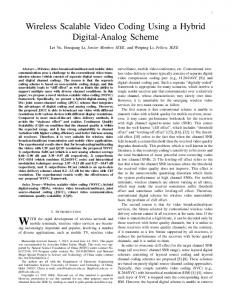
A. Architecture Design In SV-BCMCS, through SVC coding, video is encoded into one base layer and multiple enhancement layers. Viewers who receive the base layer can view the video with the minimum quality. The video quality improves as the number of received layers increases. An enhancement layer can be decoded if and only if all enhancement layers below it are received. The multicast radio channel of the base station is divided into multiple sub-channels. Different layers of video are broadcast using different sub-channels with different coverage ranges. To maintain the minimum quality for all viewers, the base layer is always broadcast using a sub-channel to cover the entire cell. To address the decoding dependency of upper layers on lower layers, the broadcast range of lower layers cannot be shorter than that of higher layers. Figure 1 depicts a simple example of SV-BCMCS with eleven multicast users and three layers of SVC video, L1, L2, and L3. The base station broadcasts three layers using three sub-channels with their respective coverage areas shown in the figure. All the users receive L1 from the base station directly, while four users receive L2 and two users receive L3 through broadcast. Using an ad-hoc network, the coverage of higher layers is extended further. User a is in the coverage of L3 and user b is in the coverage of L2. User a relays L3 to user b, who then relays L3 to users c and d. Meanwhile, user b relays L2 to users c and d. Effectively, all four users a, b, c, and d receive all three layers through the combinations of base station broadcast and ad-hoc relays.

Fig. 1.

Architecture of SV-BCMCS over a hybrid network (assuming three layers of video content).

The key design questions of the SV-BCMCS architecture are: 1) How to allocate the radio resources among sub-channels (layers) to strike the right balance between systemwide and worst-case video quality among all users? 2) How to design an efficient helper discovery and relay routing protocol to maximize the gain of ad-hoc video forwarding? 3) Given a random distribution of viewers, what is the expected performance gain brought in by ad-hoc networks? What are the major factors determining the gain? We examine these questions through analysis and simulations in the following sections. The key notation used in this paper are shown in Table I. B. Optimal Resouce Allocation in Layered Video Broadcast Our objective of radio resource allocation is to maximize the aggregate user perceived video quality while maintaining the minimum quality for all users. In video processing, Peak Signal-to-Noise Ratio (PSNR) is widely used as an indicator of video quality. There is a common belief that the higher the received video rate, the higher the PSNR, which can be verified from various theoretical and empirical studies [4], [10], [11]. Their relationship is dependent on the specific video coding schemes and is not the focus of this paper. In the following, unless otherwise noted, we use the receiving data rate as the video quality metric. However our analysis and algorithms can be easily adapted to using PSNR metrics or other general utility functions [10].

4

TABLE I N OTATION U SED IN T HIS PAPER

ri pi ni Ri L N Φ U d rt G Sc D

selected transmission rate (PHY mode) for layer i video content allocated fraction of channel for tansmission of layer i video content in 3G system number of multicast users that can receive layer i video/content in 3G domain encoding rate of an individual layer i. total number of layers total number of multicast users in the 3G domain set of all possible transmission rates (or PHY modes) aggregate data rate (utility) of users in the 3G domain distance of the user to the base station ad-hoc transmission radius/range random variable of distance gain total area of the entire 3G cell the radius of the 3G cell

Assume there are L video layers, and the video rate of each layer is a constant Ri , 1 ≤ i ≤ L. The broadcast channel is divided into L sub-channels through time-division multiplexing. Each sub-channel can operate at one of the available BCMCS PHY modes. Each PHY mode has a constant data transmission rate and a corresponding coverage range. Layer i is transmitted using sub-channel i. Let pi be the time fraction allocated to sub-channel i, and ri be the actual transmission rate, or the PHY mode, employed by sub-channel i. To support the video rate of layer i, we should have ri ∗ pi ≥ Ri . We can let pi = Rrii without affecting the optimal solution. Suppose ni multicast users can correctly receive layer i video/content, i.e., ni users’ receiving Bit-Error-Rate (BER) is lower than a specific threshold value for this rate. Therefore ni − ni−1 users, 1 ≤ i < L, receive exactly i layers of video/content, and nL users receive all L layers. The aggregate data rate for all users is: U

= (n1 − n2 ) · R1 + · · · + (nj − nj+1 ) ·

j X i=1

=

L X

ni · Ri .

Ri + · · · + nL ·

L X

Ri

i=1

(1)

i=1

For a fixed total number of multicast users N in the 3G domain, maximizing the average data rate of multicast users is the same as maximizing the aggregate data rate U in (1). Moreover, for a series of given video/content rates Ri , equation (1) indicates that it is only necessary to maximize the summation of all ni Ri , 1 ≤ i ≤ L. Next, the computation of ni is discussed. The value of ni is determined by the transmission rate ri for subchannel i. Due to path loss, fading, and user mobility, ni varies with ri and generally is a monotonically decreasing function of ri . The higher the transmission rate of the base station, the fewer the multicast users that can correctly receive the data. Thus, ni = f (ri ). That is, the number of multicast users/nodes that can correctly receive layer i is a function of the transmission rate for sub-channel i. It can be assumed that the channel can be modeled using free-space path loss model without considering fading [12]. For each transmission rate ri , the maximum coverage distance di can be derived based on the BER and SNR requirements for the PHY mode. For a given user location distribution, ni is the number of users falling into the disc centered at the base station with radius di . In a practical implementation, each user can report its average receiving data rate to the base station using the feedback channel. The base station can count ni by comparing these reported rates with the transmission rate ri . The optimal radio resource allocation problem can be formulated as the following utility maximization problem: max {ri }

U=

L X i=1

f (ri )Ri .

(2)

5

subject to: ri ≤ rj i≤j L X Ri ( ) ≤ 1. ri

and

i, j = 1, 2, · · · L.

(3) (4)

i=1

f (r1 ) = N.

(5)

ri ∈ Φ.

(6)

The objective is to find a set or transmission rates ri for each layer, to maximize the average data rate. For the constraint given by (6), Φ is the set of possible transmission rates (or PHY modes). The constraint given by (3) ensures that the coverage of lower layers is larger than that of the higher layers. Constraint (4) guarantees the sum of sub-channels is no greater than the original channel. Constraint (5) ensures that the base layer covers the whole cell to provide basic video service to all the users. Note that the traditional broadcast/multicast with one single stream becomes a special case of the above optimization problem with L = 1. C. Dynamic Programming Algorithm The optimization problem formulated above can be solved by a dynamic programming algorithm. To facilitate the design of dynamic programming algorithm, the sub-channel allocation fractions, {pi = Rrii }, are rescaled to integers. A large integer, K , is selected such that pi · K is an integer for all i. K can be 10n if all pi can be expressed using at most n significant digits. Define Uik to be the maximal utility of transmitting layer i with sub-channel fraction less than k/K , and define k Si to be the corresponding transmission rate for layer i. Then we have Uik = Sik =

max

f (ri ) · Ri

∀1 ≤ i ≤ L

(7)

argmax

f (ri ) · Ri

∀1 ≤ i ≤ L

(8)

ri ∈Φ:ri ∗k/K≥Ri ri ∈Φ:ri ∗k/K≥Ri

Uik and Sik are valued zero if the feasible set of ri is empty. Further define Uik to be the maximum utility of transmitting the first i layers (from layer 1 to layer i) with the aggregate sub-channel fraction less than k/K . Define Sjk , 1 ≤ j ≤ i to be the transmission rate for layer j corresponding to Uik . The dynamic programming algorithm is illustrated in Algorithm 1. Note the algorithm is for a general problem without considering Constraint (5). Otherwise we can replace the K in line 6 with K 0 = K(1 − Rr11 ), and resolve the solution for layer 2 ∼ L. 0 Then f (r1 ) · R1 + ULK gives the maximal utility.

Algorithm 1 Dynamic programming algorithm for sub-channel resource allocation problem 1: for k = 1 to K do 2: U1k = U1k 3: S1k = S1k 4: end for 5: for i = 2 to L do 6: for k = 1 to K do m + U k−m } 7: m ¯ = arg max{m∈[1,k] and {S m ≤S k−m or S k−m ==0}} {Ui−1 i 8: 9: 10: 11: 12: 13: 14: 15:

¯ m ¯ + U k−m Uik = Ui−1 i k− m ¯ m ¯ ∪S Sik = Si−1 i end for if Sik−m == 0 then return UiK , Sik end if end for return ULK , SLk

i−1

i

i

6

In the above algorithm, line 5 to line 14 updates Uik to include a new layer each time. Line 7 and 8 resolves the maximal utility. Line 9 expands the SLk , and here it is written as “∪” in brief. The Sik−m == 0 in line 7 and 11 indicates that no more higher layers can be included into the optimal solution, thus the program returns. Otherwise every layer will be allocated and ULK gives the optimal solution. And the optimal transmission rate for each layer i is SiK , 1 ≤ i ≤ L. The complexity of the algorithm is O(L2 K 2 ). D. Ad-hoc Video Relay: Helper Discovery and Relay Routing In a pure SV-BCMCS solution, users closer to the base station will receive more enhancement layers from the base station. They can forward those layers to users further away from the base station through ad-hoc links. Ad-hoc video relays are done in two steps: 1) each user finds a helper in its ad-hoc neighborhood to download additional enhancement layers; 2) helpers merge download requests from their clients and forward enhancement layers through local broadcast. 1) Greedy Helper Discovery Protocol: We design a greedy protocol for users to find helpers. A greedy helper discovery protocol in the 3G and ad-hoc hybrid network was first presented in [5]. In that paper every node of the multicast group maintains a list of its neighbors, containing their IDs and the average 3G downlink data rates within a time window. Users periodically broadcast their IDs and downlink data rates to their neighbors. Each user greedily selects a neighbor with the highest downlink rate as its helper. Whenever a node wants to download data from the base station, it initiates helper discovery by unicasting a request message to its helper. Then the helper will forward this message to its own helper, so on and so forth, until the ad-hoc hop limit is reached or a node with local maximum data rate is found. The ad-hoc hop limit is set by a parameter Time-To-Live (TTL) in this paper. The helpers will forward the data in the reverse direction of helper discovery to the requesting node. We employ a similar greedy helper discovery mechanism. But unlike the case considered in [5], the locations of helpers will change the resource allocation strategy of the base station in SV-BCMCS. In our scheme, the last node in the path sends the final request message to the base station. Upon receiving this message, the base station updates the 3G data rate information of all the nodes along the path as the last node’s 3G rate. After that, the base station might resolve the coverage function as f¯(ri ) = {Number of nodes with updated 3G rate above ri }. The optimal broadcast strategy can then be calculated by solving the optimization problem defined in (2). Moreover, to facilitate efficient relay routing, a node also needs to keep information about the relay requests routed through itself. The last node in the path also sends the final request message to the initiating node along the ad-hoc path. The whole process is shown in Figure 2. User C attempts to find a helper within two hops to improve its video quality. Its request goes through B to A. E and F are ignored by C and B, since they are not the neighbor with highest 3G rate. To this end, User A knows where user C is located by the reverse route of the path that user C followed to find user A. User A sends a status message to the base station to indicate that user A will act as user C ’s helper using the relay path along user B . Meanwhile, User A also sends the final request message(confirmation message) back to user C confirming that user A will act as its helper.

Fig. 2. Greedy Helper Discovery Protocol and Routing Protocol. The numbers in parenthesis are the average 3G rates for each node. The dashed line indicates the ad-hoc neighborhood. The straight solid line is the ad-hoc path with the arrow pointing to the helper. For routing protocol, dashed-dotted lines represent the coverage area of each layer. 27, 18, 12 and 5 are the physical transmission rates for layers 4, 3, 2 and 1.

7

Note that [5] also proposed another helper discovery protocol using flooding, to find the helper with the global maximal data rate within the ad-hoc hop limit range. However, considering the large overhead of flooding messages in the ad-hoc network, we only adopt the greedy helper discovery protocol within the SV-BCMCS context. 2) SV-BCMCS Relay Routing Protocol: The SV-BCMCS routing protocol executes after the greedy helper selection protocol and the optimal radio resource allocation. Assuming optimal radio resource allocation has been performed, the base station decides to transmit the L layers with different rates r1 , r2 , · · · , rL . It will broadcast this information to every node in the cell. Moreover, in the greedy helper discovery phase, each node obtains the information for all the relay paths to which it belongs by the confirmation message. The major goal of the relay routing protocol is to maximally exploit the broadcast nature of ad-hoc transmissions and merge multiple relay requests for the same layer on a common helper. Essentially, each helper needs to determine which received layers will be forwarded to its requesting neighbors. For each node n, the forwarding decision will be calculated as shown in Algorithm 2: Algorithm 2 Forwarding Algorithm in SV-BCMCS Routing Protocol for Node n 1: N ={ all node k that uses n as one-hop helper } 2: for k ∈ N do 3: Find the highest layer lk that k can directly receive from the base station 4: Find the highest layer Lk that k can expect from any potential helper 5: end for 6: lmin = min{lk , k ∈ N } 7: Lmax = max{Lk , k ∈ N } 8: node n broadcasts the packets between layer lmin + 1 to Lmax to its one-hop neighbors. Each node receives packets that satisfy two conditions: (i) the packets are sent from its direct one-hop helper; (ii) the packets belong to a layer higher than the layer to which the node itself belongs to. Otherwise the node will discard the packets. That is, the node has no use for packets that are within the layer to which the node belongs, or from a lower layer than the layer to which it belongs. A relay routing example is illustrated in Figure 2. Suppose L = 4 and maximal hop number is 2. For node B in the figure, nodes C and D use it as a direct one-hop helper. For D, lD = 2 (it is the layer to which node D belongs) according to the figure, and within 2 hops, D’s highest expected layer is LD = 4. The highest expected layer is the highest layer which a node can expect to receive through its helpers while constrained by the maximum hop count. In the same way, we can derive, lC = 1 and LC = 4. Thus, for node B, lmin = min{lC , lD } = 1 and Lmax = max{LC , LD } = 4. Therefore, node B will broadcast the packets in layers 2, 3 and 4. Node D, since it is in layer 2 and will hear the layers 2, 3 and 4 packets sent from node B, will receive packets in layers 3 and 4 only. Meanwhile, node C will receive all the packets in layers 2, 3 and 4. IV. A NALYSIS OF THE G AIN OF A D - HOC R ELAY In this section, we analytically study the expected gain from using ad-hoc relays under a random node distribution in the cell. Through ad-hoc video relays, users receiving fewer layers of packets (users at the coverage edge/boundary) are able to obtain video/content layers that they otherwise would not or could not receive. From the base station viewpoint, an ad-hoc relay shortens a user’s effective distance to the base station. As shown in Figure 2, user A relays data to user B who then relays the data to user C . Both user B and C have the same effective distance as user A. The distance gain of user C is the difference of OC and OA, where O denotes the position of the base station. In the following, we develop a probabilistic model to study the distance gain due to ad-hoc relays under a random node distribution. The typical transmission rate of an ad-hoc network, such as a network using IEEE 802.11, is much larger than the rate of a cellular network. For instance, IEEE 802.11g supports data rates up to 54 Mb/s. We therefore ignore the effect of wireless interference in our analysis. We also assume that the number of data relays, or relay hops, is small. Using only a small number of relays is more robust against user mobility, and reduces the video forwarding delay. Furthermore, a smaller number of relays also reduces the traffic volume in the whole ad-hoc network. Let G be the distance gain of an arbitrary user. Obviously, G depends on the location of the user, as well as the locations of other users in the same cell. It is also a function of the ad-hoc transmission range, and the

8

number of relay hops allowed. Denote by fG (·) the probability density function (pdf) of G. We develop a model to characterize fG (·) by assuming the users are uniformly distributed in the cell. Our approach, however, also applies to other distributions within the cell. The list of key notation is included in Table I. Figure 3 and Figure 4 depicts an arbitrary user and is used to study the user’s distance gain in the case of a one-hop and two-hop relay. 3) Distance Gain Using One-hop Relay: Assuming that the user is d distance away from the base station, and the ad-hoc transmission radius/range is rt . All other users falling into the transmission range of the user are potential one-hop helpers. Following the greedy helper discovery protocol, the user closest to the base station is chosen as the relay node. To calculate fG (g), we need to calculate the probability that the distance gain is in a small range of [g, g + ∆g].

Fig. 3.

The one-hop ad-hoc data relay of an arbitrary user

As illustrated in the Figure 3, the whole cell space is divided into three regions: S1 , S2 and S3 . Since the relay node is closer to the base station than any other node falling into the transmission range of the user, there should be no node in S2 in the Figure 3. To achieve a distance gain of [g, g + ∆g], there should be at least one node falling into S3 . Since the area of S3 is proportional to ∆g , the probability that two or more nodes fall into S3 is a higher order of ∆g , and thus will be ignored. Therefore, the probability of the distance gain in the range of [g, g + ∆g] is the probability that when we randomly drop N − 1 nodes (excluding the user under study) into the cell, one node falls into S3 , no node falls into S2 and N − 2 nodes fall into the remaining area S1 . Based on the multinomial distribution: Pr(N − 2 nodes in S1 , no node in S2 , one node in S3 ) fG (g) = lim , ∆g→0 ∆g q3 (N − 1)! q3 = lim (q1 )N −2 (q2 )0 = lim (N − 1)q1N −2 . (9) ∆g→0 (N − 2)!1!0! ∆g ∆g→0 ∆g where q1 , q2 , q3 are the probabilities of users located in the area S1 , S2 , S3 . Due to the uniform distribution of the users, qi = SSci , i = 1, 2, 3, where Sc is the area of entire cell. S2 is the overlapping area of two circles. For two circles with a known distance d12 between their centers and with radius of each circle c1 and c2 , the overlapping area can be computed. Let SII (d12 , c1 , c2 ) represent the overlapping area. The detailed derivation of SII (d12 , c1 , c2 ) is available in [13]. For our case, S2 = SII (d, rt , d − g). For a fixed rt , S2 is a function of g and d, so we use S2 (g, d) from this point on. It is easy to verify that SII (d, rt , d − g) , Sc dS2 (g, d) dSII (d, rt , x) = − = |x=d−g . dg dx

lim p1 = 1 −

∆g→0

S3 ∆g→0 ∆g lim

(10) (11)

Consequently, we have   N −1 SII (d, rt , d − g) N −2 dSII (d, rt , x) fG (g, d) = · 1− · |x=d−g . Sc Sc dx

(12)

9

The expected one-hop distance gain for a user at a distance d from the base station can be derived as: Z rt gfG (g, d)dg. µG (d) =

(13)

0

4) Distance Gain Using Two-hop Relay: The way to derive the distance gain in the two-hop case is similar to the one-hop case. However the two hop case is computationally more complex. To accurately characterize the two-hop relay gain, we need to calculate the joint density of the distance gain of the first and second relay hop. As illustrated in the right part of Figure 4, let g1 be the distance gain of the first-hop relay, θ be the angle between the first-hop helper and the user with the base station as the origin, g2 be the distance gain of the secondhop relay. In a manner similar to the one-hop case, we can calculate the joint density function f (g1 , θ, g2) by calculating the multinomial distribution of N − 1 nodes fall into five regions as illustrated in the right part of Figure 4. Let ni be the number of nodes falling into area Si . We need to calculate the multinomial probability of n1 = N − 3, n2 = n4 = 0, n3 = n5 = 1. The areas of S1∼5 are functions of g1 , g2 , d and θ.

Fig. 4.

The two-hop ad-hoc data relay of an arbitrary user

The pdf of the joint distance gain can be calculated as: S3 (N − 1)(N − 2) S5 · S1N −3 · . (14) · N −1 ∆g1 ,∆θ,∆g2 →0 ∆g2 ∆g1 ∆θ Sc P It can be determined that S5 = (d − g1 )∆θ∆g1 and S1 = Sc − 5i=2 Si . Unfortunately, the calculation of S2 , S3 and S4 is fairly involved. Now let’s take a closer look at the positions of the user, helper 1 and helper 2 in Figure 5. Note that the center positions and the radii of the circles CA , CB , CC and CD can be computed based on g1 , g2 , d, rt and θ. Going forward SII (Ci , Cj ) as the overlapping area of two circles Ci and Cj , SIII (Ci , Cj , Ck ) as the overlapping area of the three circles Ci , Cj and Ck . i, j and k are chosen from A, B, C, D in the example used herein. With known radii and center positions, the closed formulas of SII (·) and SIII (·) are derived in [13]. With different positions of the helper 2, the CD may intersect with CA and CB in three patterns shown in Figure 5. Here the results are given directly: case I: dS3 dS2 S2 = SII (CB , CD ), =− , S4 = SII (CA , CC ) (15) dg2 dg2 f (g1, g2, θ) =

lim

In case II and III, S2 and S4 overlaps with each other and combine into one part, S24 . case II: dS3 d[SII (CB , CD ) − SII (CA , CD )] =− dg2 dg2 S24 = SII (CB , CD ) + SII (CA , CC ) − SII (CA , CD )

(16)

10

Fig. 5. Reference Figure for positions of the user, helper 1 and helper 2. We label the circles as CA , CB , CC and CD , with CA and CB centered at the user and helper 1, CC and CD centered at the Base Station. I, II and III indicate the three different patterns that CD intersect with CA and CB .

case III: d[SII (CB , CD ) − SIII (CA , CB , CD )] dS3 =− dg2 dg2 S24 = SII (CB , CD ) + SII (CA , CC ) − SIII (CA , CB , CD )

(17)

The joint pdf can now be calculated as f (g1, g2, θ) =

dS3 (N − 1)(N − 2) · S1N −3 · (d − g1 ), N −1 dg2 Sc

(18)

3 with different S1 and dS dg2 as shown from (15) to (17). In case I, S1 = Sc − S2 − S4 . And in case II and III, S1 = Sc − S24 . Finally, the expected two-hop distance gain for user at the distance d can be calculated as Z g2∗∗ µG1 +G2 (d) = Φ(III) (g1, g2, d, θ)dg2 0 Z g2∗ Z rt Φ(I) (g1, g2, d, θ)dg2 (19) + Φ(II) (g1, g2, d, θ)dg2 +

g2∗

g2∗∗

with Z

rt

Z

θ∗

Φ(i) (g1, g2, d, θ) = 0

−θ∗

(g1 + g2 )fG1 G2 (i) (g1, g2, d, θ)dθdg1 , i = I, II, III

(20)

The critical values of g2 from case I to II and case II to III are defined as g2∗ and g2∗∗ . Moreover, according to the law of consines, we have: d2 + (d − g1 )2 − r2 θ∗ = arccos (21) 2d(d − g1 ) 5) Impact of ad-hoc wireless relay to user performance: With the aid of ad-hoc wireless relay, the video layers can be received by more users. In other words, more users “appear to exist” within certain distance of the base station compared to the scenario with no ad-hoc relay. Next we derive the number of users that effectively move closer to the base station with the use of ad-hoc wireless relay. As shown in Figure 6, our objective is to calculate on average how many users outside a given distance d can move into the circle, with the aid of ad-hoc relay. The increase represents the number of additional users that can receive a certain video layer. We divide the ring between a distance d and d + rt into many concentric rings, each with a width of 4. Note that rt is the range of ad-hoc transmission. One-hop ad-hoc relay is considered in this case; however the approach can be applied to the multiple hop relay scenario. N is the total number of multicast users in the entire cell, and D is the radius of the cell. The average number of users in the k th ring is:

11

Fig. 6.

The impact of ad-hoc video relay to user performance

4[(2k − 1)4 + 2d] π[(d + k4)2 − (d + (k − 1)4)2 ] =N . 2 πD D2 Then, the probability that a user in the k -th ring can move within distance d is: Z rt fG (g, d)dg pk (4) = Nk (4) = N ·

(22)

k4

The average number of users that moves into the circle of radius d is: b r4t c

Nave =

X

Nk (4) · pk (4).

(23)

k=1

As 4 → 0, Equation (23) can be rewritten as: Z Nave (d) = 0

rt

2N (d + r) D2

Z

rt

fG (g, d)dg dr.

(24)

r

Recall in our formulation (2), with the assistance of the ad-hoc network, the base station can reach a larger number of users f¯(ri ) ≥ f (ri ). Now f¯(ri ), expressed as f¯(ri ) = f (ri ) + Nave (di ), where di , the distance for certain transmission rate ri , can be derived. 6) Numerical Results Using the Analytical Model: Based on the analytical model presented above, we numerically computed the resulting distance gain and user number increase. Since the pdf is a function of d, the user achieves different distance gain when its distance to the base station varies. The results in this section are for different node densities in a 3G cell with a radius 1000 meters. We set the ad-hoc range at 100 meters. Therefore, if there are a π1002 totally 500 nodes, on average each node has 500 · π1000 2 = 5 neighbors. Figure 7 shows how the distance gain g derived in section IV-3 and IV-4 changes with d when TTL is set to one and two. For example, when the total number of multicast users is 700, for the user at the boundary of the cell, i.e, d = 1000, the expected one-hop and two-hop distance gains are gT T L=1 = 62.86 and gT T L=2 = 121.61. For the same setting with 500 multicast users, we calculate the increase in the numbers of users at different ranges according to Equation (23). For d = 500, 700 and 900 meters, the “number increase/original number of users” are 28.57/125, 38.32/245, 48.08/405 respectively. Note without ad-hoc, the original number of users goes proportional to d2 due to the uniform user distribution. We can observe an obvious increase as ad-hoc relay squeezes the users towards the base station. This explains the potential of video quality improvement by using ad-hoc network in the SV-BCMCS protocol. V. P ERFORMANCE E VALUATION In this section, the performance of SV-BCMCS is evaluated using OPNET based simulations. The performance of SV-BCMCS is compared with the performance of traditional 3G BCMCS under various scenarios. The impact of node density, node mobility, number of relay hops and base layer video rate is investigated, as well as the fairness issue. Results demonstrate that SV-BCMCS consistently out-performs BCMCS with or without the aid of ad-hoc data relay.

12

130

The Average Distance Gain (meters)

120

110

100

600 nodes, one−hop 600 nodes, two−hop 500 nodes, one−hop 500 nodes, two−hop 400 nodes, one−hop 400 nodes, two−hop

90

80

70

60

50

40 100

200

300

400

500

600

700

800

900

1000

Distance to the Base Station (meters)

Fig. 7.

The one-hop and two-hop Distance Gain for nodes with different distance to the base station.

A. Simulation settings SV-BCMCS is simulated using the wireless modules of OPNET modeler. It is assumed that all multicast users/nodes have two wireless interfaces: one supports a CDMA2000/BCMCS channel for 3G video service, and the other supports IEEE 802.11g for ad-hoc data relay. The data rate of the ad-hoc network is set to be 54 Mb/s, and the transmission power covers 100 meters. Since OPNET modeler does not have wireless modules with dual interfaces, the 3G downlink is simulated as if individual users generate their own 3G traffic according to the experimental data presented in [1], [14]. The free-space path loss model is adopted for 3G downlink channels, where the Path Loss Exponent (PLE) is set to be 3.52, and the received thermal noise power is set to be -100.2dBm. Eleven PHY data rates are supported according to the 3GPP2 specifications [15]. The 3G cell is considered to be a circle with a radius of 1000 meters, with a base station located in the center. It is assumed that 3G BCMCS supports a video streaming rate of 153.6 kb/s. According to [1], 153.6 kb/s can be supported in almost 100 percent of the coverage area using a Reed-Solomon error correction code. The transmission power of the 3G base station is set accordingly so that BCMCS can broadcast the video to the entire cell. The same base station transmission power is used in SV-BCMCS evaluations. Constant Bit Rate (CBR) video is used in the simulations with a packet size of 1024 bytes. A user’s average receiving data rate is used as an indicator of the user’s received video quality. B. Stationary Scenarios In stationary scenarios, a certain number of fixed nodes are uniformly distributed in the 3G cell. The presented results are averages over ten random topologies. The 90% confidence interval is also determined for each simulation point. 1) The Impact of Node Density: In this scenario, we fix the base layer rate to 100 kb/s and each enhancement layer rate to 64 kb/s, with the video consisting of one base layer and five enhancement layers. We use (100, 64 ∗ 5) to represent this layered video stream and all the scenarios will use this setting, unless specified otherwise. The number of multicast nodes in the cell is ranging from 100 to 600, to simulate a sparse to dense node distribution. “Traditional BCMCS” indicates the transmission of a 153.6 kb/s single layer video, covering the whole cell. The average data rates for scenarios without an ad-hoc network, and scenarios with ad-hoc network (TTL set to 3), are given in Figure 8. Table II lists the average data rates and the percentage gain for SV-BCMCS with/without ad-hoc network and different numbers of users. We can see from the table that the SV-BCMCS with (100, 64 ∗ 5) setting provides up to a 76.85% average data rate gain compared to traditional BCMCS. Without ad-hoc, the optimal allocation in

13

Average Received Data Rates (kb/s)

280

260

240

220

200

SV−BCMCS with ad−hoc SV−BCMCS without ad−hoc Traditional BCMCS

180

160

140

100

200

300

400

500

600

Number of Multicast Receivers Fig. 8.

Node density impact: average receiving data rate. TABLE II DATA R ATE C OMPARISON FOR D IFFERENT N ODE D ENSITY ( KB / S )

Node No. 100 200 300 400 500 600

Single Stream 153.6 153.6 153.6 153.6 153.6 153.6

SV-BCMCS without ad-hoc 210.24 (36.88%) 211.53 (37.72%) 206.11 (34.19%) 209.11 (36.14%) 204.68 (33.20%) 207.35 (34.96%)

SV-BCMCS with ad-hoc 220.16 (43.33%) 232.71 (51.50%) 244.51 (59.18%) 258.93 (68.55%) 267.83 (74.35%) 271.64 (76.85%)

SV-BCMCS can support around a 36% improvement. The ad-hoc network delivers a larger performance gain when the node density increases. When the number of nodes is 100, it gives an 6.46% additional improvement, while when the node number is 600, the additional improvement reaches 41.89%. 2) The impact of number of relay hops (TTL): Figure 9 depicts the performance of SV-BCMCS under different TTLs. The analysis in Section IV shows the effective distance gain of users with the aid of ad-hoc data relay. Here the impact of ad-hoc relay is examined in a more practical setting - with a larger number of relay hops and in the presence of wireless interference. The experiments are done with the number of users set to be 300 and 600, respectively. They represent different node density levels, with the former one sparse and the latter one dense. With TTL=1 and 300 users, the average receiving data rate is 47.71% higher than the rate supported in traditional BCMCS. The improvement percentage increases to 64.26% when the TTL reaches four. Ad-hoc relays achieves better performance with more users in the cell. A higher user density leads to a larger probability of connecting to a helper, hence a higher video rate. With TTL values ranging from one to four in the 600 users scenario, the data rate improvement percentage rises from 52.17% to 88.16%, respectively. Note that with TTL=0, no ad-hoc relay is used. In this case, SV-BCMCS still out-performs BCMCS by 36.15%. C. Mobile Scenarios The impact of user mobility to the users’ received video rate is studied next. The random walk model with reflection mobility [16] is used to drive user movement in the simulation. The individual user’s moving speed is randomly selected in a range from zero to maxspeed (m/s), where maxspeed is a simulation parameter. Both moving speed and moving direction are adjusted periodically, with the time period drawn from a uniform distribution

14

Average Received Data Rates (kb/s)

300

280

260

240

220

SV−BCMCS with ad−hoc: 600 nodes SV−BCMCS with ad−hoc: 300 nodes Traditional BCMCS

200

180

160

140

120 −0.5

0

0.5

1

1.5

2

2.5

3

3.5

4

4.5

Time−To−Live (TTL) of the ad−hoc network Fig. 9.

TTL impact: average received data rate.

between zero and 100 seconds. The mobility affects SV-BCMCS’s performance in the following two aspects: (i) the efficiency of ad-hoc network degrades due to the link failures caused by mobility, and (ii) the optimal channel allocation is disrupted since the user positions keep changing. SV-BCMCS periodically reconfigures the optimal allocation so as to adapt to the change in user positions. 1) Impact of moving speed: There are 600 users in the cell, with ad-hoc relay hops (TTL) set to three. The maxspeed is set at 2, 5, 10, 15, 20 and 30 m/s, respectively. The base station reconfiguration interval of the optimal channel allocation is set to be 30 seconds. Again, six video layers are used with a base layer rate of 100 kb/s and enhancement layer rate of 64 kb/s. Figure 10 depicts the average receiving rates for different maxspeed. Clearly, the performance of the SV-BCMCS degrades as the users move faster, especially when the speed increases beyond 15 m/s. In fact, when the speed is above 15 m/s, the average received data rates are approaching the values without the aid of ad-hoc data relay, as shown in Section V-B.

Average Received Data Rates (kb/s)

300

SC−BCMCS in Mobile Scenario SC−BCMCS in Static Scenario 280

260

240

220

200

180

160

2.0

5.0

10.0

15.0

20.0

Speed of the Mobile Nodes (m/s) Fig. 10.

The impact of maxspeed on average data rate.

30.0

15

TABLE III I MPACT OF R ECONFIGURATION I NTERVAL ON THE AVERAGE RECEIVED R ATE (maxspeed=10 M / S )

Reconfiguration Interval (sec) Average Received Rate (kb/s)

45 218.46

30 229.67

15 243.34

5 264.99

2) The Impact of the Reconfiguration Interval: Table III summarizes the impact of optimal allocation reconfiguration interval on the average receiving data rate when maxspeed is 10 m/s. When the interval becomes shorter, the SV-BCMCS can adapt to the mobile environment faster, leading to better performance. This is at the price of computing power and communication overhead. D. Fairness Issue In SV-BCMCS, depending on a user’s location, it may receive the same video at different quality levels by receiving a different number of video layers. In the worst case, a user may only receive the base layer, which is transmitted to the entire cell. SV-BCMCS allows users having better channel condition to receive better quality video, which is “fair” to some degree. The study of the right fairness metric, however, is outside the scope of this paper. Here we focus on the tradeoffs between the base layer rate and the overall improvement of user perceived video quality. Figure 11 depicts the average receiving data rate vs. the base layer rate in SV-BCMCS with and without ad-hoc data relay. The enhancement layer rate is fixed to 64 kb/s. The average receiving data rate remains high when the base layer rate is less than 80 kb/s. As the base layer rate increases further, the average receiving data rate decreases. The base layer rate must not exceed the single layer rate (153.6 kb/s) as used in BCMCS. At this rate, the entire channel can only transmit the base layer, and there is no difference between SV-BCMCS and BCMCS. Intuitively, the high base rate leaves less “room” for SV-BCMCS to optimize and to achieve a higher average data rate.

Average Received Data Rates (kb/s)

320

SV−BCMCS with ad−hoc TTL=3 SV−BCMCS without ad−hoc 300

280

260

240

220

200

180 60

70

80

90

100

110

120

The Base Layer Encoding Rate (kb/s) Fig. 11.

Impact of Base Layer Encoding Rate on the average received data rate.

Figure 12 shows the average receiving data rate versus the distance to the base station in SV-BCMCS. Six layers are used and the base layer rate is set to be 80 kb/s and 120 kb/s, respectively. The rates of enhancement layers are set to be 75 kb/s. There are 600 users in the cell. Vertical lines indicate the transmission ranges of different video layers. Notice that several layers may be transmitted to cover the same range. Each point in the figure represents one user. Clearly, more users in the small base rate case (base layer rate of 80 kb/s) are able to enjoy higher data rate (> 153.6 kb/s) than in the large base rate case (base layer rate of 120

16

550

Average Received Data Rate (kb/s)

(80, 75 * 5) setting 500

450

400

SV−BCMCS nodes not using ad−hoc Edge distance of layer 6 Edge distance of layer (4,5) Edge distance of layer (2,3) SV−BCMCS nodes using ad−hoc Traditional BCMCS

350

300

250

200

150

50

LayerLayer 4,5 2,3

Layer 6

100

0

100

200

300

400

500

600

Layer 1

700

800

900

1000

Distance to the Base Station (meter)

550

SV−BCMCS nodes not using ad−hoc Edge distance of layer (2,3,4) SV−BCMCS nodes using ad−hoc Traditional BCMCS Edge distance of layer 5

Average Received Data Rate (kb/s)

(120, 75 * 5) setting 500

450

400

350

300

250

200

150

100

50

Layer 2,3,4

Layer 5 0

100

200

300

400

500

Layer 1 600

700

800

900

1000

Distance to the Base Station (meter) Fig. 12. Fairness issue in SV-BCMCS. Optimal resource allocation significantly improves the system-wide video rate at the price of a small rate decrease for nodes close to the boundary; ad-hoc relays further increase the rate for all users, almost all users achieve a higher video rate than in the traditional BCMCS.

kb/s). When using less channel bandwidth to deliver a smaller rate base layer, enhancement layers are transmitted further. However, the users who only obtain the base layer perceive worse video quality in the small base rate case than in the large base layer rate case. With the aid of ad-hoc data relay, more users are able to receive higher data rate regardless of the base layer rate. VI. C ONCLUSION In this paper we present SV-BCMCS, a novel scalable video broadcast/multicast solution that efficiently integrates scalable video coding, 3G broadcast and ad-hoc forwarding. We formulate the resource allocation problem for scalable video multicast in a hybrid network and propose a dynamic programming algorithm to achieve the optimal solution. Efficient helper discovery and video forwarding schemes are designed for practical layered video/content dissemination through ad-hoc networks. Furthermore, we analyze the distance gain enabled by ad-hoc relay, which provides insight into the video quality improvement made possible by using ad-hoc data relay. Finally, OPNET simulations show that a practical SV-BCMCS increases the average receiving video rate by 76.85%, with the

17

ad-hoc networks accounting for 41.89% improvement. Moreover, SV-BCMCS still maintains a minimum of 50% performance improvement when the nodes’ moving speed is less than 5 m/s, while periodical reconfiguration is necessary in fast moving scenarios. The fairness issue is discussed and we demonstrate that SV-BCMCS can significantly improve the system-wide video quality, though a few viewers close to the boundary will have a slight rate degradation. R EFERENCES [1] P. Agashe, R. Rezaiifar, and P. Bender, “CDMA2000 High Rate Broadcast Packet Data Air Interface Design,” IEEE Commun. Mag., vol. 42, no. 2, pp. 83–89, February 2004. [2] J. Wang, R. Sinnarajah, T. Chen, Y. Wei, and E. Tiedemann, “Broadcast and Multicast Services in CDMA2000,” IEEE Commun. Mag., vol. 42, no. 2, pp. 76–82, February 2004. [3] “Third Generation Partnetship Project (3GPP2).” [Online]. Available: http://www.3gpp2.org/ [4] H. Schwarz, D. Marpe, and T. Wiegand, “Overview of the Scalable Video Coding Extension of the H.264/AVC Standard,” IEEE Trans. Circuits Syst. Video Technol., vol. 17, no. 9, pp. 1103–1120, September 2007. [5] H. Luo, R. Ramjee, P. Sinha, L. E. Li, and S. Lu, “UCAN: A Unified Cellular and Ad-Hoc Network Architecture,” in Proc. of ACM MOBICOM, 2003. [6] H. Hsieg and R. Sivakumar, “On Using Peer-to-Peer Communication in Cellular Wireless Data Networks,” IEEE Trans. Mobile Comput., vol. 3, no. 1, pp. 57–72, February 2004. [7] J. C. Park and S. K. Kasera, “Enhancing Cellular Multicast Performance Using Ad Hoc Networks,” in Proc. of IEEE Wireless Comm. and Networking Conf. (WCNC), 2005. [8] R. Bhatia, L. E. Li, H. Luo, and R. Ramjee, “ICAM: Integrated Cellular and Ad Hoc Multicast,” IEEE Trans. Mobile Comput., vol. 5, no. 8, pp. 1004–1015, August 2006. [9] K. Sinkar, A. Jagirdar, T. Korakis, H. Liu, S. Mathur, and S. Panwar, “Cooperative Recovery in Heterogeneous Mobile Networks,” in Proc. of IEEE SECON, 2008. [10] M. Chen, M. Ponec, S. Sengupta, J. Li, and P. A. Chou, “Utility Maximization in Peer-to-Peer Systems,” in Proc. of ACM SIGMETRICS, 2008. [11] T. Kim and M. H. Ammar, “A comparison of heterogeneous video multicast schemes: Layered encodign or stream replication,” IEEE Trans. Multimedia, vol. 7, no. 6, pp. 1123–1130, 2005. [12] A. Goldsmith, Wireless Communications. Cambridge University Press, 2004. [13] M. Fewell, “Area of Common Overlap of Three Circles,” Tech. Rep. DSTO-TN-0722, 2006. [Online]. Available: http: //hdl.handle.net/1947/4551 [14] P. Bender, P. Black, M. Grob, R. Padovani, N. Sindhushayana, and A. Viterbi, “CDMA/HDR: A Bandwidth Efficient High Speed Wireless Data Servicefor Nomadic Users,” IEEE Commun. Mag., vol. 38, no. 7, pp. 70–77, July 2000. [15] “CDMA2000 High Rate Broadcast-Multicast Packet Data Air Interface Specification,” 3GPP2 Specifications, C.S0054-A v1.0 060220, February 2006. [16] T. Camp, J. Boleng, and V. Davies, “A Survey of Mobility Models for Ad Hoc Network Research,” Wireless Communications and Mobile Computing (WCMC), vol. 2, no. 5, pp. 483–502, 2002.