back line is a spray root line. Assuming that a spray root line is straight, the wetted surface area of a prismatic planing surface model is expressed by Eq. (1),.
Proceedings of AP Hydro 2002,pp.7--14
DEVELOPEMENT OF RESISTANCE TEST FOR HIGH-SPEED PLANING CRAFT USING VERY SMALL MODEL - SCALE EFFECTS ON DRAG FORCE Toru KATAYAMA*1, Shigeru HAYASHITA*2, Kouji SUZUKI*1 and Yoshiho IKEDA*1 *1Department of Marine System Engineering, Osaka Prefecture University Sakai, JAPAN 2 * Department of Naval Architecture, Nagasaki Institute of Applied Science Nagasaki, JAPAN
ABSTRACT In order to develop a resistance test method for high speed planing craft using a very small model, the scale effects on wetted surface area, frictional resistance and pressure forces acting on a small model are experimentally investigated using geosim prismatic planing surface models. Froude number and Renolds number covered in the experiments are Fn=1.0 to 4.0 and Rn=5×10⁵ to 3×10⁶, respectively. Through the analysis of resistance components, it is found that a resistance component created by removal of hydrostatic pressure on the transom due to high-speed, called transom pressure resistance in the paper, plays an important role in the resistance of a planing craft. The wetted surface area is confirmed to slightly decrease for a very small model at large trim angle, and to cause the reduction of the pressure force acting on the hull. The frictional resistance acting on a very small model can be predicted on the basis of the equivalent flat plate concept if appropriate prediction formulas, in which laminar and transient flow effects are taken into account, are used. KEY WORDS: High-Speed Planing Craft, Resistance test, Scale effects, Drag Force, Lift Force, Frictional Resistance, Residual Resistance, Transom Stern INTRODUCTION In towing tanks, the common method of resistance tests using a scale model ship is that the resistance and running attitudes of a towed model in the state of heaving and pitching freedom are measured. In order to satisfy the relation of Froude’s law of similarity in the resistance test for a high-speed planing craft, it is necessary to use a very small model. If the length of model is shorter than 1.5 m, however, it was pointed out by DTNSRDC(1981), Tanaka
et al (1991) and ITTC (1987)(1990)(1999) that scale effects on running attitudes appears and causes different resistance. Therefore a model longer than 1.5 m is recommended to use in the resistance tests for a planing craft. On the other hand, if a larger model is used, a towing carriage should run very fast. Then a very long tank with a very fast towing carriage is needed. Furthermore, the wall and bottom effects may appear in resistance. In the previous paper published by Hayashita et al (2002), the authors proposed two prediction methods for resistance and attitudes of a craft using a very small model, which can overcome these problems mentioned above. One method uses a simulation method proposed by Yokomizo et al (1992) and Ikeda et al (1995), in which the running attitude and resistance are calculated by solving the balance equations for the vertical forces and trim moments acting on a running ship, using a database of measured hydrodynamic forces acting on a fully captured model. In the database, the scale effects on the forces and moments are taken into account. Another one is the new experimental method proposed by Hayashita (1995)(1996)(1999) that measures the running attitude and resistance of a small model by adding the forces and moments to compensate the scale effects. In the both methods, it is important to take the scale effects on hydrodynamic forces and moments into consideration. In the previous paper, the hydrodynamic forces acting on the two geosim high-speed craft models, one of which is a very small model of a 0.47m length, were measured, and it was pointed out that the scale effects on lift force and trim moment as well as resistance force should be taken into account. In this study, in order to clarify the scale effects on the hydrodynamic forces acting on a very small model, the hydrodynamic forces acting on three geosim prismatic planing surface models are measured at high speed (Fn=1.0 to 4.0, Rn=5×10⁵ to 3×10⁶) for four trim angles (3, 4, 6 and 9 degrees).
EXPERIMENTAL PROCEDURE Model and Experimental Procedures Models used in the experiments are geosim prismatic planing surface models with constant deadrise angle β=20 degrees. The prismatic model is selected because the measured hydrodynamic force can be easily divided into two components, a pressure force component and a frictional force component. A body plan and their principle particulars are shown in Fig.1 and Table 1. The experimental setup is shown in Fig.2. The model is captured by a 3-component load cell, and towed in the towing tank (70 m × 3 m × 1.6 m) of Osaka Prefecture University by an unmanned carriage, the maximum speed of which is 15 m/s. Drag and lift forces and trim moment acting on the model are measured. Zero levels of all the forces are set at rest just before starting of the carriage. Wetted surface areas at running condition are taken by photographs with a digital video camera installed above the model, which has a transparent bottom.
Table 1 Principal particulars of geosim prismatic planing surface models. Model Length: LOA Breadth: B Depth: D Deadrise angle: β Wetted keel length at rest: LK Trim angle: τ
M-90 0.90 0.21 0.18 0.645 0.745 3, 4, 6, 9
M-60 M-30 0.60 0.30 m 0.14 0.07 m 0.12 0.06 m 20 degrees 0.430 0.215 m 0.497 0.248 m 3, 4, 6, 9 9 degrees
0.12 (m)
0.08
0.04
–0.05
0 0
Table 2 Average of measured force, precision index and precision index of average for M-30. 0.05 (m)
towing speed
Fig.1 Body plan of geosim prismatic planing surface models (Scale for M-60). lift(+) FZ drag(+) FX
trim moment(+) MY
CCD forward speed (+) U
load cell
τ LK
Fig.2
In this experiments, trim angle τ are systematically changed, but for all trim angles the wetted keel length at rest LK are constant as shown in Table 1. Towing speeds U are also systematically changed. Although the models are very small, no turbulence flow generator is fitted. Uncertain Analysis of Experimental System The precision of the experiment system used in the present study is explained in this section. At 15 m/s of the maximum speed of the towing carriage, the deviation from the setting speed is 3.475×10⁻⁴ m/s, the standard deviation is 0.0161. The results show that the precision of the speed control of the towing carriage is considered to be accurate enough. In the measurement of the hydrodynamic forces acting on a fully captured model, we must be especially careful for seiche of a towing tank that significantly affects on the measured value of the lift force acting on a model. In the towing tank used in the experiments, the first order period of the seiche is about 35.5 seconds. After the experiments with generating waves, water surface elevation by the seiche is measured. The results show that its amplitudes is about 1.0 mm in 10 minutes, about 0.5 mm in 16 minutes, and about 0.3 mm in 25 minutes after the finish of the experiment, respectively. On the basis of these results, the interval time between measurements is decided to be about 20 minutes. The results of the uncertainty analysis of measured hydrodynamic forces for M-30 are shown in Table 2. A sampling frequency for data acquisition is set to be 50 Hz and a 20 Hz low path filter is used. Measurement ranges of the forces and moment are about 15 kgf and 7 kgfm, and the resolution of an AD translator is 16 bits. The results shown in Table 2 demonstrate that the precision index and the precision index of average are less than 5 % of the average values of measured forces.
Schematic view of fully captive model test.
1.4 m/s 5.7 m/s MY(kgfm) -0.0050 -0.1148 average FZ(kgf) 0.0793 1.4663 value FX(kgf) 0.0369 0.3456 MY(kgfm) 0.0159 0.0205 precision FZ(kgf) 0.0613 0.1199 index FX(kgf) 0.0683 0.0864 precision MY(kgfm) 0.00002 0.0016 index of FZ(kgf) 0.00007 0.0093 average FX(kgf) 0.00008 0.0067
14 m/s -0.6613 9.6459 2.2442 0.1391 0.1743 0.5895 0.0220 0.0275 0.0932
SCALE EFFECTS ON WETTED SURFACE AREA In this paper, the wetted surface area is defined as the area over which water pressure is exerted, and geometrically bottom area aft of spray root line. Photo.1 shows an example of measured spray field. In the photograph, two lines can be clearly seen on the bottom of a model. Hirano (1994), from the result of the detailed investigation to the photographs taken by the same way, indicated that the front line is a spray edge line and that the back line is a spray root line. Assuming that a spray root line is straight, the wetted surface area of a prismatic planing surface model is expressed by Eq. (1), 0.5(LKU + LC )B SS = cos β
Fig.5 shows the comparison among the measured wetted keel lengths for the three models at trim angle of 9 degrees. The length of M-30 is about 5 % shorter than those of other two larger models.
Forward speed Still water line Spray root line
chine keel
(1) LW
where LKU is a wetted keel length at running condition and LC is wetted chine length at running condition as shown in Fig.3. From photographs taken in the similar way to the case of Photo.1, spray root lines of the geosim models used here are obtained. Some examples of the results, in which the scale effect clearly appears, are shown in Fig.4. The results demonstrate that at 6 m/s of a forward speed no difference between the lines for different scale models appears but at 2 m/s the spray root line of the smallest model, M-30, goes back. The experimental results also suggest that the scale effects on a wetted surface area at running condition appear only if a trim angle is large and the wetted surface area decreases when a model is very small. The predicted results by Savitsky’s empirical formula are shown in same figure. The formula is expressed as follows. B tan β π tan τ d = LK = sin τ
LKU − LC =
(2)
LKU
(3)
The results are in fairly good agreement with the measured results for M-90 and M-60, but in poor agreement with those for M-30 in relatively low speed (2 m/s in Fig.4) and at large trim angle (9 degrees).
LC LK
Fig.3 Waterline intersection for constant deadrise surface.
U=2 m/s M–90 M–60 M–30 Savitsky
Chine line
Fig.4
L KU /LK 1.2
U=6 m/s
L KU /LK 1.2
1.1
1.1
1.0
1.0
0.9
0.9
0.8
0.8
0.7
0.7
0.6
0.6
Keel line
Chine line
Keel line
Measured spray root lines of geosim models.
LKU /LK 1
0.5
Spray root line 0 0
Spray edge line
Photo.1 Photograph of spray field.
M–90 M–60 M–30
LK /B=3.55
2
4 Fn=U/√(gL OA)
Fig.5 Wetted keel length LKU with forward speed at LK/B=3.55 at τ=9 degrees.
SCALE EFFECTS ON FRICTONAL RESISTANCE Deduction of Frictional Resistance Fig.6 show examples of measured drag FX (horizontal direction) and lift FZ (vertical direction) acting on M-60 by a load cell. From these forces, tangential force component FKT and normal force component FKN to keel line are obtained by Eqs. (4) and (5). FKT = FX cos τ − FZ sin τ
FKN = F X sin τ + FZ cos τ
(4) (5)
It should be noted that the tangential force component FKT consists of frictional component acting on the bottom and hydrodynamic pressure force acting on the flat transom. At rest, hydrostatic pressure acts on the transom. At high speed, however, the hydrostatic pressure acting on the transom is replaced by air pressure since transom is exposed into the air. Then the removed force can be regarded as an additional resistance. This resistance is proportional to the third power of scale. For a prismatic planing surface model, this resistance FKTS can be calculated as follows, B
FKTS = 2 ∫ 2 0
Obtained FKT and FKN are shown in Fig.7.
= ρg ( Fx (kgf) :τ=9deg. :τ=6deg. :τ=4deg. :τ=3deg.
4
2
0 0
2
4 Fn=U/√(gL OA)
Fz (kgf) 20
∫
LK tan τ − y tan β
0
ρgz cos τdzdy
B3 B2 tan 2 β − LK tan τ tan β 24 4 B 2 + L K tan 2 τ ) cos τ . 2
(6)
(7)
where ρ is mass density of fluid, g is acceleration due to gravity, B is breadth of waterline, β is deadrise angle of a planing surface,τ is trim angle and LK is wetted keel length at rest. In Fig.8, the proportions of the resistance obtained by Eq. (7) to the total tangential force to keel line FKT are shown. The results demonstrate that the resistance due to removal of hydrostatic pressure on the transom FKTS occupies 20 to 70 % in the total tangential force FKT and that it can not be disregarded. Particularly this component is dominant at larger trim angle and in a relatively low-speed region. In the present paper the resistance component will be called ‘transom pressure resistance’.
10
FKTS /FKT 1
0 0
Fig.6
2
:τ=9deg. :τ=6deg. :τ=4deg. :τ=3deg.
4 Fn=U/√(gL OA)
Measured drag and lift forces of M-60 at LK=0.43 m.
0.5
FKT (kgf) 1
:τ=9deg. :τ=6deg. :τ=4deg. :τ=3deg.
0 0
4 Fn=U/√(gL OA)
Fig.8 Proportion of transom pressure resistance FKTS to total tangential resistance FKT of M-60 at LK=0.43 m.
0.5
0 0 FKN (kgf)
2
2
4 Fn=U/√(gL OA)
20
10
As pointed out by many researchers, aerodynamic force FKTair acting on a part of a model above water line may play an important role in resistance tests of high-speed craft. The tangential force FKT includes the aerodynamic force component FKTair, too. The component FKTair can be predicted by the following Eq.(8), FKTair = 0.5 ρSU 2 C D × cos τ
0 0
2
4 Fn=U/√(gL OA)
Fig.7 Tangential and normal forces to keel line of M-60 at LK=0.43 m.
(8)
where S is front projection area of the part of a model above water line and CD is the drag coefficient. Assuming that the drag coefficient CD is constant (CD=1.0 is used here) at any forward speed, this force is proportional to the third power of scale. In Fig.9, the proportion of the force to the
total tangential force FKT is shown. The results demonstrate that the aerodynamic force FKtair occupies about 15 % in the total tangential force FKT in the present experiments. The frictional resistance Rf is obtained by subtracting the transom pressure resistance FKTS and the aerodynamic force FKTair from the total tangential force FKT as Eq. (9). R f = FKT − ( FKTS + FKTair )
2
Pd =
4 Fn=U/√(gL OA)
Fig.9 Proportion of air resistance component FKTair to total tangential force FKT of M-60 at LK=0.43 m. Frictional Resistance Coefficient In order to predict the frictional resistance using the equivalent flat plate concept commonly used, the frictional resistance coefficient Cf is presented by in Eq.(10) after Savitsky (1964), Cf =
Rf 0.5 ρS S V A
(10)
2
where SS is wetted area at running and VA is average bottom velocity. As pointed out by many researchers, real wetted surface area at running condition should be used as SS in Eq. (10). In the present calculation, Savisky’s empirical formula Eqs.(1) to (3) are used to predict the wetted surface area. In Fig.10, the proportions of the predicted wetted area SS at running to the wetted area SF at rest are shown. The wetted surface area SS at running condition is larger than the area SF at rest and increases with decreasing trim angle.
2
(11)
where U is forward velocity. Pd is average dynamic pressure that is obtained by dividing the total normal force to keel line FKN by the wetted surface area at running condition SS as Eq. (12).
:τ=9deg. :τ=6deg. :τ=4deg. :τ=3deg.
0 0
1 1 ρV A 2 + Pd = ρU 2 2 2
(9)
FKTair/FKT 1
0.5
According to the proposal of Savitsky (1964), applying Bernoulli’s equation between the free-stream condition and the average pressure and velocity conditions on the bottom of a planing surface, the average bottom velocity can be obtained by Eq. (11),
FKN SS
(12)
In Fig.11, the proportion of the average bottom velocity VA obtained by Eq. (11) to the forward velocity U is shown. The results demonstrate that the average bottom velocity VA is smaller than the forward velocity U, and for larger trim angles the difference between the average bottom velocity VA and the forward velocity U becomes larger. The Reynolds number Rn of the models is defined as Eq. (13), ( L + LC ) V A KU VAλA B 2 Rn = = (13)
ν
ν
where ν denotes kinematic viscosity of fluid. VA /U 1
0.95
0.9 0
β=20deg. λ=3.07
2
:τ=3° :τ=4° :τ=6° :τ=9° 4 Fn=U/√(gL OA)
Fig.11 Ratio of average bottom velocity to forward speed for M-60 at LK=0.43 m.
SS/SF
Characteristics of Frictional Resistance The frictional resistance coefficients of M-60 obtained by the present experiments are shown in Fig.12. In the figures, the predicted lines by Schoenherr’s method for turbulent flow, that by Blasius’s method for laminar flow and that by Plandtl’s method for transient flow are shown, too.
SS 1
SF
LK=0.43m β=20deg. 0 0
5
trim angle(deg.)
10
Fig.10 Proportion of wetted pressure area at running condition SS to wetted area SF at rest of M-60 at LK=0.43 m.
Laminar flow, Rn≤5.3×10⁵ (Blasius): C f = 1.328 Rn −0.5
(14)
Transient flow, 5.0×10⁵