o Estimation of fundamental matrix in stereo. ⢠Structure ... For further details, refer to Section 3.4 of the book on Digital Image Processing by Gonzalez, or see the ...
Scale Invariant Feature Transform (SIFT) CS 763 Ajit Rajwade
What is SIFT? • It is a technique for detecting salient, stable feature points in an image. • For every such point, it also provides a set of “features” that “characterize/describe” a small image region around the point. These features are invariant to rotation and scale.
Motivation for SIFT • Image matching o Estimation of affine transformation/homography between images o Estimation of fundamental matrix in stereo • Structure from motion, tracking, motion segmentation
Motivation for SIFT • All these applications need to (1) detect salient, stable points in two or more images, and (2) determine correspondences between them. • To determine correspondences correctly, we need some features characterizing a salient point. • These features must not change with: o Object position/pose o Scale o Illumination o Minor image artifacts/noise/blur
Motivation for SIFT • Individual pixel color values are not an adequate feature to determine correspondences (why?).
Motivation for SIFT • One could try matching patches around the salient feature points – but these patches will themselves change if there is change in object pose or illumination. • So these patches will lead to several false matches/correspondences.
Motivation for SIFT • SIFT provides features characterizing a salient point that remain invariant to changes in scale or rotation. Extract affine regions
Normalize regions
Eliminate rotational ambiguity
Compute appearance descriptors
SIFT (Lowe ’04)
Image taken from slides by George Bebis (UNR).
Steps of SIFT algorithm • Determine approximate location and scale of salient feature points (also called keypoints) • Refine their location and scale • Determine orientation(s) for each keypoint. • Determine descriptors for each keypoint.
Step 1: Approximate keypoint location • Look for intensity changes using the difference of Gaussians at two nearby scales: Convolution operator: refers to the application of a filter (in this case Gaussian filter to an image)
Difference of Gaussians = “DoG”. Scale refers to the σ of the Gaussian.
0.0049 0.0092 0.0134 0.0152 0.0134 0.0092 0.0049
0.0092 0.0172 0.0250 0.0283 0.0250 0.0172 0.0092
0.0134 0.0250 0.0364 0.0412 0.0364 0.0250 0.0134
0.0152 0.0283 0.0412 0.0467 0.0412 0.0283 0.0152
0.0134 0.0250 0.0364 0.0412 0.0364 0.0250 0.0134
0.0092 0.0172 0.0250 0.0283 0.0250 0.0172 0.0092
0.0049 0.0092 0.0134 0.0152 0.0134 0.0092 0.0049
This is a 7 x 7 (truncated) Gaussian mask with mean zero and standard deviation σ = 2.
Convolution means the following (non-rigorously): Let the original image be A. Let the new image be B. You move the mask all over the image A. Let us suppose the mask is centered at location (i,j) in image A. You compute the pointwise product between the mask entries and the corresponding entries in A. You store the sum of these products in B(i,j).
B(i, j )
r
r
A(i a, j b) M (a, b)
a rb r
Whenever you are performing a filtering operation on image, the resultant image is obtained by convolving the original image with the filter, and is said to be the response to the filter. For further details, refer to Section 3.4 of the book on Digital Image Processing by Gonzalez, or see the animation at: http://en.wikipedia.org/wiki/Convolution
http://www.gimpbible.com/files/edge-detection-difference-of-gaussians/
This is an example of the DoG filter in gimp. In SIFT, however, the DoG is computed from Gaussians at nearby scales.
Step 1: Approximate keypoint location Downsampling
D( x, y, ) L( x, y, k ) L( x, y, )
L ( x, y , ) G( x, y, )* I ( x, y)
Octave = doubling of σ0. Within an octave, the adjacent scales differ by a constant factor k. If an octave contains s+1 images, then k = 2(1/s). The first image has scale σ0, the second image has scale kσ0, the third image has scale k2σ0, and the last image has scale ksσ0. Such a sequence of images convolved with Gaussians of increasing σ constitute a so-called scale space.
Scale = 0
Scale = 1
Scale = 4
Scale = 16
Scale = 64
Scale = 256
http://en.wikipedia.org/wiki/Scale_space
Step 1: Approximate keypoint location Image taken from D. Lowe, “Distinctive Image Features from Scale-Invariant Points”, IJCV 2004
The keypoints are maxima or minima in the “scale-space-pyramid”, i.e. the stack of DoG images. Hereby, you get both the location as well as the scale of the keypoint.
Initial detection of keypoints
http://upload.wikimedia.org/wikipedia/commons/4/44/Sift_keypoints_filtering.jpg
Step 2: Refining keypoint location • The keypoint location and scale is discrete – we can interpolate for greater accuracy. • For this, we express the DoG function in a small 3D neighborhood around a keypoint (xi,yi,σi) by a second-order Taylor-series: T
D( x, y , ) 1 T 2 D ( x, y , ) D( x, y , ) D( xi , yi , i ) ; 2 xx , x x , i 2 ( x, y , ) y yi , ( x, y , ) y yi , i i
x xi y yi i
Gradient vector evaluated digitally at the keypoint
i
3 x 3 Hessian matrix evaluated digitally at the keypoint
Step 2: Refining keypoint location • To find an extremum of the DoG values in this neighborhood, set the derivative of D(.) to 0. This gives us: xˆ 1 2 D ( x, y , ) D( x, y , ) ˆ y ( x, y , ) 2 x xi , ( x, y , ) x xi , y yi , y yi , ˆ i i xˆ 1 D( x, y , ) D( xi , yi , i ) yˆ x x , 2 ( x, y , ) y yii , i ˆ T
Dextremal
• The keypoint location is updated. • All extrema with |Dextremal| < 0.03, are discarded as “weak extrema” or “low contrast points”.
Removal of low-contrast keypoints
http://upload.wikimedia.org/wikipedia/commons/4/44/Sift_keypoints_filtering.jpg
Step 2: Refining keypoint location • Some keypoints reside on edges, as edges always give a high response to a DoG filter. • But edges should not be considered salient points (why?). • So we discard points that lie on edges. • In the case of KLT tracker, we saw how to detect points lying on salient edges using the structure tensor.
Step 2: Refining keypoint location • The SIFT paper uses the 2nd derivative matrix (called the Hessian matrix):
• The eigenvalues of H give a lot of information about the local structure around the keypoint. • In fact, the eigenvalues are the maximal and minimal principal curvatures of the surface D(x,y), i.e. of the DoG function, at that point. http://en.wikipedia.org/wiki/File:Minimal_surface_curvature_planes-en.svg http://en.wikipedia.org/wiki/Principal_curvature
Step 2: Refining keypoint location • An edge will have high maximal curvature, but very low minimal curvature. • A keypoint which is a corner (not an edge) will have high maximal and minimal curvature. • The following can be regarded as an edge-ness measure:
Should be less than a threshold (say 10). For an edge, α >> β, leading to a large value of this measure. Why this measure instead of r? To save computations – we need not compute eigenvalues!
Removal of high-contrast keypoints residing on edges
http://upload.wikimedia.org/wikipedia/commons/4/44/Sift_keypoints_filtering.jpg
Step 3: Assigning orientations • Compute the gradient magnitudes and orientations in a small window around the keypoint – at the appropriate scale.
35
Histogram of gradient orientation – the bin-counts are weighted by gradient magnitudes and a Gaussian weighting function. Usually, 36 bins are chosen for the orientation.
30
25
20
15
10
5
0 -0.5
0
0.5
1
1.5
2
2.5
3
3.5
Step 3: Assigning orientations • Assign the dominant orientation as the orientation of the keypoint. • In case of multiple peaks or histogram entries more than 0.8 x peak, create a separate descriptor for each orientation (they will all have the same scale and location). 35
Histogram of gradient orientation – the bin-counts are weighted by gradient magnitudes and a Gaussian weighting function. Usually, 36 bins are chosen for the orientation.
30
25
20
15
10
5
0 -0.5
0
0.5
1
1.5
2
2.5
3
3.5
Step 4: Descriptors for each keypoint • Consider a small region around the keypoint. Divide it into n x n cells (usually n = 2). Each cell is of size 4 x 4. • Build a gradient orientation histogram in each cell. Each histogram entry is weighted by the gradient magnitude and a Gaussian weighting function with σ = 0.5 times window width. • Sort each gradient orientation histogram bearing in mind the dominant orientation of the keypoint (assigned in step 3). Image taken from D. Lowe, “Distinctive Image Features from Scale-Invariant Points”, IJCV 2004
Step 4: Descriptors for each keypoint • We now have a descriptor of size rn2 if there are r bins in the orientation histogram. • Typical case used in the SIFT paper: r = 8, n = 4, so length of each descriptor is 128. • The descriptor is invariant to rotations due to the sorting. Image taken from D. Lowe, “Distinctive Image Features from ScaleInvariant Points”, IJCV 2004
Step 4: Descriptors for each keypoint • For scale-invariance, the size of the window should be adjusted as per scale of the keypoint. Larger scale = larger window. Image taken from D. Lowe, “Distinctive Image Features from Scale-Invariant Points”, IJCV 2004
http://www.vlfeat.org /overview/sift.html
Step 4: Descriptors for each keypoint • The SIFT descriptor (so far) is not illumination invariant – the histogram entries are weighted by gradient magnitude. • Hence the descriptor vector is normalized to unit magnitude. This will normalize scalar multiplicative intensity changes. • Scalar additive changes don’t matter – gradients are invariant to constant offsets anyway. • Not insensitive to non-linear illumination changes.
Step 1: Keypoint computations? (More details) • Why are DoG filters used? • The Gaussian filter (and its derivatives) is shown to be the only filter obeys all of the following: Linearity Shift-invariance Structures at coarser scales are related to structures at finer scales in a consistent way (smoothing process does not produce new structures) Rotational symmetry Semi-group property: G( x, y,1 ) * G( x, y, 2 ) G( x, y,1 2 ) + some other properties http://en.wikipedia.org/wiki/Scale_space
Step 1: Keypoint computations? (More details) • Why difference of Gaussians? The DoG is an approximation to the scalemultiplied Laplacian of Gaussian filter in image processing – a rotationally invariant filter. The DoG is a good model for how neurons in the retina extract image details to be sent to the brain for processing.
LoG filter of scale σ produces strong responses for patterns of radius σ * sqrt(2).
http://www.cs.utexas.edu/~grauman/courses/spring2011/slides/lecture14_localfeats.pdf
Keypoint = center of blob
http://www.cs.utexas.edu/~grauman/courses/spring2011/slides/lecture14_localfeats.pdf
http://www.cs.utexas.edu/~grauman/courses /spring2011/slides/lecture14_localfeats.pdf
http://www.cs.utexas.edu /~grauman/courses/spring 2011/slides/lecture14_loc alfeats.pdf
http://www.cs.utexas.edu /~grauman/courses/spring 2011/slides/lecture14_loc alfeats.pdf
Gxx Gyy
Isotropic heat equation: running this equation on an image is equivalent to smoothing the image with a Gaussian. Numerical approximation
Step 1: Keypoint computations? (More details) • Why do we look for extrema of the DoG function? Maxima of the DoG indicate dark points (blobs) on a bright background. Minima of the DoG indicate bright points (blobs) on a dark background. • Why do we look for extrema in a spatial as well as scale sense? It helps us pick the “scale” associated with the keypoint!
Step 1: Keypoint computations? • How many scales per octave? Answer: 3 – it is empirically observed that this provides optimal repeatability under downsampling/upsampling/rotation of the image as well as image noise.
Image taken from D. Lowe, “Distinctive Image Features from Scale-Invariant Points”, IJCV 2004
Step 1: Keypoint computations? • Adding more scales per octave will increase the number of detected keypoints, but this does not improve the repeatability (in fact there is a small decrease) – so we settle for the computationally less expensive option.
Summary of SIFT descriptor properties • Invariant to spatial rotation, translation, scale. • Experimentally seen to be less sensitive to small spatial affine or perspective changes. • Invariant to affine illumination changes. Image taken from D. Lowe, “Distinctive Image Features from Scale-Invariant Points”, IJCV 2004
Application: Matching SIFT descriptors • Given a keypoint descriptor in image 1, find its nearest neighbor in image 2. “Nearest” as defined typically by SSD: rn2
d (a1 , a2 ) (a1 (i ) a2 (i ))2 i 1
I1
I2
• Threshold the distance to decide whether the matching pair was valid.
Application: Matching SIFT descriptors • May lead to many false matches.
Application: Matching SIFT descriptors • Consider the match between the keypoints to be valid if and only if the second nearest neighbor distance (SNND) in image 2 is sufficiently larger than the nearest neighbor distance (NND). • Accept match as valid if SNND/NND > 0.8 (see next slide).
Image taken from D. Lowe, “Distinctive Image Features from Scale-Invariant Points”, IJCV 2004
Application: Object Recognition • Input (1): A reference database of images of various objects. Each image is labeled by object name and object pose + scale. • Input (2): Query images in which you locate one or more of these objects.
Application: Object Recognition • Compute and store keypoints and their descriptors for each image in the reference database. • Compute keypoint descriptors for the query image. • For each keypoint, find the nearest matching descriptor in each image of the reference database subject to the SNND/NND constraint.
Application: Object Recognition • Collect all keypoints in the query image that “vote for” a particular pose for object X in the reference database. • “Vote for pose abc of object X” = “have a nearest neighbor in image of object X with pose θ (say)”
Application: Object Recognition • Estimate an affine transformation between keypoint locations (xi,yi) from the query image and keypoint locations (ui,vi) for each candidate reference image.
• Verify the affine transformation: apply the transform to the keypoints and compute the difference between the transformed and target locations. Discard the point as an outlier if the difference between the orientations/scales/locations is too high.
Application: Object Recognition • What is too high? Orientation difference > 20 degrees Scale difference more than 1.5 Location difference > 0.2 * size of model • Repeat the solution for affine transformation until no more points are thrown out. • If number of points < 3, affine transformation cannot be estimated.
SIFT: ++ • Resistant to affine transformations of limited extent (works better for planar objects than full 3D objects). • Resistant to a range of illumination changes • Resistant to occlusions in object recognition, since SIFT descriptors are local.
SIFT: • Resistance to affine transformations is empirical – no hard-core theory provided. • Several parameters in the algorithm: descriptor size, size of the region, various thresholds – theoretical treatment for their specification not clear.