Scaling Laws for Data-Centric Storage and Querying in ... - USC

1

Scaling Laws for Data-Centric Storage and Querying in Wireless Sensor Networks Joon Ahn, Student Member, IEEE, and Bhaskar Krishnamachari, Member, IEEE

Abstract—We use a constrained optimization framework to derive scaling laws for data-centric storage and querying in wireless sensor networks. We consider both unstructured sensor networks, which use blind sequential search for querying, and structured sensor networks, which use efficient hash-based querying. We find that the scalability of a sensor network’s performance depends upon whether or not the increase in energy and storage resources with more nodes is outweighed by the concomitant application-specific increase in event and query loads. We derive conditions that determine (i) whether or not the energy requirement per node grows without bound with the network size for a fixed-duration deployment, (ii) whether or not there exists a maximum network size that can be operated for a specified duration on a fixed energy budget, and (iii) whether the network lifetime increases or decreases with the size of the network for a fixed energy budget. An interesting finding of this work is that 3D uniform deployments are inherently more scalable than 2D uniform deployments, which in turn are more scalable than 1D uniform deployments. Index Terms—Energy efficiency, Modeling, Performance analysis, Querying, Scalability, Wireless sensor networks

I. I NTRODUCTION

W

IRELESS sensor networks are envisioned to consist of large number of embedded devices that are each capable of sensing, communicating, and computing. While the network as a whole is required to provide fine resolution monitoring for an extended period of time, the individual embedded devices face some fundamental constraints. They are typically deployed with limited battery supplies and, because of their form factor and low cost, may also have limited data storage capability. The goal of this research is to understand the conditions under which a query-based data-centric sensor network [1] deployed in various dimensions can be operated in a scalable manner despite these constraints on energy and storage. We consider both unstructured and structured varieties of data-centric querying along with replicated storage in this research. In unstructured querying schemes, the node issuing the query does not know in advance where any copy of the requested event information can be found. The query dissemination is therefore a form of blind search (this can take the form of an expanding ring search or a sequential trajectory search). In structured querying schemes, a hash or index is used so that the querying node knows exactly where the nearest copy of the requested event information can be found. In This work was supported in part by the NSF through the NETS-NOSS grant 0435505, CAREER grant 0347621, and ITR grant CNS-0325875. J. Ahn and B. Krishnamachari are with the Ming Hsieh Department of Electrical Engineering, University of Southern California, Los Angeles, CA, 90089 USA (e-mail: {joonahn, bkrishna}@usc.edu)

such networks, there is a trade-off between the energy costs of replicated storage and querying that is determined by the number of replicas created for each event. A large number of replicas results in lowered query cost at the expense of greater storage cost, and vice versa. We first formulate an optimization problem whose aim is to select the optimal number of replicas that minimizes the total energy cost of querying and storage. We use this optimization problem as a tool to identify the conditions, in terms of the numbers of events and queries, under which query resolution can be performed in a scalable manner despite constraints on energy. Practically, the storage available on the sensor nodes is limited, so the optimization problem should also consider this as a constraint. It turns out, though, that the storage constraints are less restrictive than the energy constraints. We therefore first derive the scalable operating conditions using an unconstrained version of the optimization problem, and then use the constrained version to investigate in more detail the behaviors of the network as its size grows. We find that operating a network in a scalable fashion essentially requires that the traffic load due to additional events and queries be outweighed by the improvement in energy and storage resources obtained as the network size increases. Note that the scaling of event and query activity with network size is application specific — e.g., in many applications there may be only a constant number of queriers regardless of the network size, but the number of events detected grows linearly with the covered area; in other applications, the number of querying nodes may increase in some fashion with the network size, while the events detected remain constant. Thus, our results suggest that only certain types of applications are inherently scalable, while others are not. Another interesting finding is that networks deployed in higher dimensions are inherently more scalable. Thus, 3D uniform deployments are inherently more scalable than 2D uniform deployments, which in turn are more scalable than 1D uniform deployments. Intuitively, this happens because in higher dimensions the same number of nodes can be packed within a smaller diameter, resulting in a lower average energy consumption per store/query operation. In this paper we consider a fixed-radius, constant-density node deployment model in which it is ensured that the network remains connected regardless of size. Hence, it is important to note that our analysis does not cover the commonly-studied case of uniform random deployment, as this requires logarithmically increasing neighbor density to ensure connectivity with high probability [21]–[23]. However, grid-like and other regularized random deployments ensuring a bounded distance between nodes would satisfy our model. One justification for

2

not considering uniform random deployments in our analysis is that this kind of deployment explicitly rules out the kind of scalability we are interested in exploring. In the uniform random deployment case, with a fixed spatial density of nodes, √ the radio range needs to be increasing as d log N as the network size N increases in order to maintain connectivity. Thus, a finite per-node energy budget can never sustain an arbitrarily large deployment of this kind. In the case of constant radio range that we examine, however, we show that there are conditions under which such scalability is still possible. The rest of the paper is organized as follows. We present related work in section II, and state our basic assumptions in section III. In section IV we formulate the unconstrained optimization problem that is at the core of our analysis. We then examine the asymptotic energy costs associated with the optimal solution in section V to identify the application growth conditions under which the energy requirement remains bounded. In section VI, we show how the network size can vary with the available energy resources per node for different regimes of application load. We then examine how the network lifetime is affected by network size for different application conditions in section VII. We incorporate storage constraints into the optimization framework and address scaling under storage constraints in section VIII. The hot-spot problem is discussed in section IX. We discuss about relaxed replication schemes and their effects on the scaling laws in section X. Finally, we present concluding comments in section XI. II. R ELATED W ORKS There have been many interesting studies on the scalability of the wireless networks in terms of throughput [3]–[8]. Many of them have focused on the upper bounds on the throughput from the information-theoretic point of view (that is, without any particular assumption on the way communications take place) using order notation, while Li et al. [8] has focused on the feasible throughput of the network using the 802.11 MAC protocol. However, our study investigates the scalability in another domain, namely, energy consumption, because energy is among the most precious resources in wireless sensor networks. Some prior studies have looked at maximizing the energy efficiency in order to increase the lifetime of wireless sensor networks [9]–[12]. But, they have focused on controlling the network topology given parameters such as network size. Some other studies have looked at the asymptotic energyconstrained network lifetime [13] or maximizing the network lifetime [14]–[16]. However, these studies pertain to continuous data-gathering applications; our focus here is on datacentric in-network storage and querying, which is an important paradigm for sensor networks. As for the analytical modeling of query strategies which we deal with to deduce our scaling laws, there have been several interesting prior studies [17]–[20]. The energy costs of data centric storage are compared with the two extremes of external storage and local storage in [17]. A hybrid push-pull

query processing strategy is proposed and analyzed in [18]. Shakkotai [19] has presented a comparison of the asymptotic performance of three random walk-based query strategies, showing that a rendezvous-based sticky search has the best success probability over time. The optimal parameter setting for the comb-needles approach is analyzed in [20]. An analytical comparison of the comb-needles approach and data centric storage is provided in [27]. However, these studies have not developed scaling laws for data-centric storage and querying. Further, all these prior studies do not address the question of application-specific conditions that determine limits on scalability of sensor networks. To our knowledge this is the first work on the topic. III. A SSUMPTIONS The following are the key assumptions in our work: • N nodes are deployed with a fixed radio range R and a constant density in a d-dimensional ball Bd space. The constant density implies that if the network size is increased, the deployment area grows proportionally. We further assume that the deployment methodology ensures connectivity. • The sensor network is deployed for a fixed applicationspecific time duration T . This assumption is relaxed in section VII when we investigate the scalability of network lifetime. • During this time duration, there are m atomic events that are sensed in the environment. The distribution of events is assumed to be uniform in the deployment area. • A total of ri copies of each event i are maintained with a uniform distribution in the network by creating ri − 1 additional replicas when the event is first sensed. • For each event i, there are a total of qi queries that are generated uniformly by the nodes in the network. Each query is an one-shot query (i.e. requires a single response, not a continuous stream), and is satisfied by locating a single copy of the corresponding event. • We assume that the links over which transmissions take place are lossless (e.g., using blacklisting) and present no interference due to concurrent transmissions (e.g., due to low traffic conditions or due to the use of a scheduled MAC protocol). • The total energy cost for storage and querying is assumed to be proportional to the total number of transmissions. This is reasonable particularly for sleep-cycled sensor networks where radio idle times are kept to a minimum. • We assume that the storage at each node is a constant amount s, so that the total storage S = s · N , where each event copy requires a unit of storage. IV. BASIC O PTIMIZATION A. Modeling Querying and Replication Costs We now turn to developing mathematical models to quantify the cost of replication and search. We consider two types of data-centric querying techniques: structured and unstructured. In structured environments, the information is stored in the network and retrieved from it using a hash. This approach

3

is exemplified by the geographic hash-table technique [2]. Thus, in structured querying, the querying node is aware of the location of the nearest copy of the replicated event information and sends the query directly to this point to get a response. In unstructured environments, by contrast, there is no predetermined location where the querying node can send a query. Hence the query must be disseminated through a form of blind search. If latency is not a concern, efficient unstructured querying strategies involve expanding ring searches or sequential trajectories [24], [25]. The detailed derivations of the querying and replication costs in either structured or unstructured network are presented in Appendix. Since we are interested in the scalability in terms of the order of the size of network, we present below instead some approximate first-order modeling with intuitive explanations for how these costs vary as a function of the network size N and the number of copies r, for a given event. First consider the replication costs. In both the structured and unstructured case these are same. The average number of hops from random event locations in the network to random √ locations is proportional to d N (since the N nodes are placed uniformly in Bd ). Thus the cost of creating and placing r − 1 replicas at random locations in the network from random event locations is: √ d Creplication = c1 · N · (r − 1) (1) The replication cost can be reduced using an enhanced replication scheme, which may exploit the fact that the event information is exposed to the set of intermediate nodes in the path anyway when a query is replied. The details of this situation are discussed in section X. Let us then consider the search cost for a structured environment. If the number of copies of the target event is kept fixed, since the copies are placed uniformly in the network, the distance (in hops) between the querying node to the nearest √ copy increases with the network size as proportional to d N . If, on the other hand, the network size is kept fixed, then as the number of copies increases and continues to be placed in the d-dimensional area with a uniform distribution among the N nodes, the expected one-dimensional distance to the nearest √ copy decreases inversely proportional to d r. Thus we have the following: √ d N Csearch,structured = c2 · √ (2) d r Finally, let us consider the search cost for an unstructured environment. The search is analogous to looking sequentially for the first of r specific objects of a desired type from a randomly ordered set of N total objects. It can be shown that the expected number of steps till the first object of the desired type is observed is given as: Csearch,unstructured

N = c3 · r+1

(3)

We have also derived special version of the above expressions for two-dimensional network in previous work [26], [27]. We have shown in the paper that the expressions are valid even for the 2-dimensional grid network.

We note that in calculating the search costs we have not explicitly taken into account the cost to return the response back to the querying node. For the structured scheme, this is easy to incorporate as the response is returned along the reverse path as the directed query, and hence incorporating this cost is equivalent to simply doubling the cost (which can be absorbed into the constant term). For the unstructured scheme, √ d N ) the cost of a directed response will be of the order O( √ d r and hence, for the large networks that are the focus of this   N study, negligible compared to the O r+1 cost of the blind search. Looking at (1), (2), and (3), we find that, as expected, the replication costs increase with the number of replicas, while the search costs decrease with the number of replicas. We can resolve this tradeoff by considering the aggregate total expected cost of search and replication and optimizing for it. The following is the common form of the total cost: Ct =

m X

qi Cs (ri ) +

m X

c2

m X

Cr (ri )

(4)

i=1

i=1

where Cs (ri ) is the expected search cost of ith event and Cr (ri ) is its expected replication cost. From the above, we get the following expressions for the expected total energy cost for all events which consists of search costs weighed by the number of queries and the replication costs: 1) Under the unstructured replication scheme, the total energy cost is Ct,u =

i=1

m X √ N qi d c1 N (ri − 1) + ri + 1 i=1

2) Under the structured replication scheme √ m m d X N qi X √ d c3 √ Ct,s = c1 N (ri − 1) + d r i i=1 i=1

(5)

(6)

To simplify our expressions, with a slight abuse of notation, we shall make the following substitutions: in (5), after dividing both sides by c1 , we let Ct,u /c1 → Ct,u and cc21 qi → qi ; in (6), after dividing both sides by c1 , we let Ct,s /c1 → Ct,s and c3 c1 qi → qi . And the following expressions are the simplified versions; m m X X √ N qi d + N (ri − 1) r + 1 i i=1 i=1 m √ m d X N qi X √ d = N (ri − 1) + √ d r i

Ct,u =

Ct,s

i=1

(7)

(8)

i=1

B. Optimization Formulation Now we can formulate the problem of optimizing the total cost as follows; P Pm Minimize Ct = m (9) i=1 qi Cs (ri ) + i=1 Cr (ri )

We use the total energy cost in the network as the object function instead of per-node energy for the optimization. Although naive replication-query schemes might make the

4

system behave differently depending on which point of view is taken (total energy or per-node energy), the system behaviors for both point of views could be essentially same (in terms of O-notation) with a smarter replication-query scheme as discussed in section IX. Moreover, the use of total energy gives at least the upper bound for the network scalability condition for any replication-query scheme. We also ignore the storage constraints for now because it turns out that the constraints must not be active in order to ensure the scalability of the network. In section VIII we incorporate the constraints to investigate more detailed behavior of the network as it grows. The optimization formulation does require global knowledge of query rates for each event and hence the optimum may not be necessarily achieved by distributed heuristics in practice, but this is still a useful tool for our investigation of performance scalability as it provides the best-case scenario. For global optimization first-order conditions are sufficient because it can be shown that the objective functions for both the unstructured and structured scheme are convex. Solving these conditions, we find that ( 1/2 d−1 (unstructured) (10a) qi N 2d − 1, ∗ ri = d d+1 (structured) (10b) βs qi , where

d

βs = d− d+1

(11)

Now we can derive the optimal expected total energy costs substituting (10a) and (10b) into (7) and (8) respectively as follows; m   X √ d+1 √ d ∗ N 2d qi − N Ct,u = 2 (12) i=1

∗ Ct,s

=

m X

− 1√ d

βs

d

d d+1

Nqi

i=1 m √ X d

+

i=1

V. C ONDITIONS

  d d+1 N βs qi − 1

FOR

(13)

d+1 2d

≥

1 d

for all d ≥ 1.

Theorem 2 (Total Cost of Structured Networks): The total energy cost for structured networks grows with network size N as follows:   d 1 ∗ (15) Ct,s = Θ m · q d+1 · N d Proof: It can be proven in the same way as the proof of Theorem 1 using (13)

To understand the implications of these theorems, it is helpful to consider some extreme cases of the scaling behavior of the number of events m and the query rate q. We consider allowing each of these parameters to scale as Θ(1) or Θ(N ), giving us four possible combinations. In practice the scaling behavior of the events and queries with network size is determined by the application scenario. For instance, an application which requires the network (regardless of its size) to have only a single sink injecting queries for events would have that q is Θ(1), while a richer application involving increasing numbers of users with the network size could have that Θ(N ). For many event monitoring applications, it is likely to be reasonable to assume that the number of observed events scales proportionally with the deployment area which for a constant density deployment would mean that m is Θ(N ); however in other applications the scaling of m may be weaker, all the way down to the extreme of Θ(1) (which would imply that there only a finite number of events that can be detected regardless of the network size). The following table exhibits the scaling of total energy costs for the four cases under the unstructured networks. Table I: Illustration of the scaling of total energy costs for unstructured networks. H HH m Θ(1) Θ(N ) HH q Θ(1) Θ(N )

Θ(N Θ(N

d+1 2d

)

2d+1 2d

Θ(N

)

Θ(N

3d+1 2d 4d+1 2d

) )

S CALABILITY

In order to obtain useful insights regarding scalability, we simplify our expressions from this point on by assuming that the query rates for all events are uniform, i.e., qi = q, ∀i. We now examine the scaling behavior of the total energy costs for both unstructured and structured networks. Theorem 1 (Total Cost of Unstructured Networks): The total energy cost for unstructured networks grows with network size N as follows:   d+1 √ ∗ (14) Ct,u = Θ m · q · N 2d Proof: The total energy cost is given from (12) by, m   X √ √ d+1 √ d+1 √ d d N 2d qi − N = 2m qN 2d − 2m N 2 i=1

The last equality holds since

  √ d+1 = Θ m qN 2d

We generate a similar table below using Theorem 2 to illustrate the scenarios for structured networks. Table II: Illustration of the scaling of total energy costs for structured networks. HH m Θ(1) Θ(N ) HH q H Θ(1) Θ(N )

1

Θ(N d ) Θ(N

d2 +d+1 d2 +d

Θ(N )

Θ(N

d+1 d

)

2d2 +2d+1 d2 +d

)

We observe something striking about Tables I and II. In both tables, among the four cases, only when both q and m are Θ(1) do we observe that the total costs for the whole network scale as O(N ) for all dimension. In other words, only in this example case do we have O(1) scaling of the pernode cost, i.e. bounded energy consumption per node. This

5

motivates us to inquire about the general conditions under which a network can scale while ensuring that the energy requirement per node is kept bounded — a very important requirement from a practical perspective. Theorem 3 (Scalability Condition of Unst’d Networks): For unstructured networks, the energy requirement per node is bounded if and only if  d−1  m · q 1/2 is O N 2d

Proof: The total optimal energy cost per node is the total cost divided by the number of nodes N . If the energy requirement per node is bounded, there exists C0 > 0 such that, from the per-node total cost given from (12) divided by N (assuming qi = q, ∀i), 1−d

1−d

Since

∗ Ct,u /N = 2mq 1/2 N 2d − 2mN d ≤ C0   C 1−d d−1 0 ⇒ m · q 1/2 − N 2d ≤ N 2d 2

1−d 2d

≤ 0 so that N

1−d 2d

≤ 1, for q ≥ 4,

q 1/2 − N

1−d 2d

(16)

1

≥1

(17)

Hence, 1−d mq 1/2 ≤ m(q 1/2 − N 2d ) 2  d−1  ⇒ mq 1/2 = O N 2d  d−1  Conversely, if mq 1/2 is O N 2d ,

(18) (19)

d−1

mq 1/2 ≤ C0 N 2d   1−d d−1 ⇒ m · q 1/2 − N 2d ≤ C0 N 2d ⇒ 2mq 1/2 N

1−d 2d

− 2mN

1−d d

≤ 2C0

(20)

Note that the left side of inequality (20) is equal to the optimized per-node total energy cost. Therefore, the per-node total energy cost is bounded. Theorem 4 (Scalability Conditions of Structured Networks): For structured networks, the energy requirement per node is bounded if and only if  d−1  d m · q d+1 is O N d

Proof: It can be proven in the same way as the proof of Theorem 3 using (13). d−1

d−1

We note that both N 2d and N d from the above scalability conditions are increasing functions with respect to the dimension d. Therefore, we can see that networks deployed in higher dimensions are inherently more scalable. 1 It can be proven for all q > 0, but the proof would be unnecessarily long and clumsy because ri∗ in (10) becomes less than 1 which means we need to correct ri∗ to be one because ri is at least one and the total cost is convex; therefrom, we need to make several trivial changes. We omit the corresponding proof due to the limited space and assume that q ≥ 4 is reasonable enough.

VI. N ETWORK S CALING

ON

F IXED E NERGY B UDGET

We now consider having a fixed energy budget, and look into what conditions the network size must satisfy to ensure that events and queries within the finite deployment time duration can be resolved before energy depletion. Specifically, we will assume that there is an average energy budget e for each node, so that the total energy is E = e · N . Definition 1: We say a network operates successfully if it can satisfy all queries for all events in a given deployment period before energy depletion. This requires that Ct ≤ e · N . The last case of each of the following two theorems has subcategories the proofs of which need to borrow knowledge in section VIII. We provide the subcategorization here for the sake of self-completeness of the theorems. Theorem 5 (Network Scaling on Fixed Energy Budget): Given a fixed average per-node energy e (i.e., the total energy allocated optimally among the nodes in the network grows linearly with the network size as E = e · N ), the following statements describe the conditions on the network size N , network dimension d, the number of events m and the number of queries per event q that ensure that the network can be operated successfully. d−1

1) If mq 1/2 is o(N 2d ) for unstructured networks d d−1 (mq d+1 = o(N d ) for structured networks), then there exists a minimum network size Nmin (e) beyond which it can always be operated successfully. d−1 2) If mq 1/2 is Θ(N 2d ) for unstructured networks d d−1 (mq d+1 = Θ(N d ) for the structured), then there exists an average per-node energy e∗ such that for all e < e∗ , it is not possible to operate a network of any size successfully, while for all e ≥ e∗ it is possible to operate a network of any size successfully. d−1 3) If mq 1/2 is ω(N 2d ) for unstructured networks d d−1 (mq d+1 = ω(N d ) for the structured), then there exists a maximum network size Nmax (e) beyond which the network cannot be operated successfully. Further, a) If mq 1/2 is o(N ) for unstructured networks d 2d (mq d+1 = o(N d+1 ) for the structured), then Nmax is a convex function of e b) If mq 1/2 is Θ(N ) for unstructured networks 2d d (mq d+1 = Θ(N d+1 ) for the structured), then Nmax increases linearly with e. c) If mq 1/2 is ω(N ) for unstructured networks d 2d (mq d+1 = ω(N d+1 ) for the structured), then Nmax increases as a concave function of e. Proof: The proof is given in Appendix. Fig. 1 illustrates the network size versus energy budget curves for the 2-dimensional deployment; the five cases are for the different cases in Theorem 5. The other dimensional networks, particularly those of one and three dimension, exhibit similar behavior. The figure is obtained numerically by equating the expressions for total cost with the energy

6

(a)

(b)

(c)

(d)

(e)

Fig. 1: Network size conditions for successful operation with respect to the per-node energy budget for different event-rate and query-rate scaling behaviors, for a 2D unstructured network; S denotes the successful region while U denotes the unsuccessful region. (a) case 1 of Theorem 5, (b) case 2, (c) case 3.a, (d) case 3.b, and (e) case 3.c

budget E = e · N , and solving for N as a function of e, under particular m and q scaling settings that satisfy each of the corresponding cases. (A very similar figure can be obtained for structured networks and is omitted due to lack of space). The regions marked S and U are where the network operates successfully and unsuccessfully, respectively. We see that under case 1, there is a minimum network size that is needed to ensure successful operation, and this minimum network size decreases rapidly with increasing energy availability. In this case, the event and query activity remains low enough that adding nodes to the network is beneficial (as it increases the available total energy). Under the event-query activity case 2, there exists an per-node energy threshold such that below this threshold, no network can operate successfully, but beyond this threshold, networks of any size can be operated. Under cases 3.a, 3.b, and 3.c, we see that for a given energy budget there exist maximum network sizes beyond which successful operation is impossible. In these cases, adding nodes to the network is harmful as each additional node introduces more consumption than resources. The key distinction between these cases is that under case 3.a, there is a convex growth that implies that adding energy resources to each node provides a super-linear improvement in the maximum network size that can be sustained; under case 3.b, the maximum network size grows linearly with the pernode energy budget; and under case 3.c, the concave growth of the curve implies that adding energy resources provide diminishing returns in maximum network size. VII. S CALING I MPLICATION IN T ERMS N ETWORK

OF

L IFETIME

OF

We now consider a relaxation of one of our key assumptions — that the network is being operated for a fixed duration. This allows us to examine how the lifetime of the network (the period over which all queries for all events can be resolved successfully) scales with the network size. In this connection we will assume that the total number of events since network initiation and the total number of queries per event (m(t), q(t)) are such that they are both non-decreasing functions of time, and at least one is a strictly increasing function of time.

T case 1

case 2

case 3

N

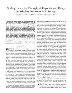
Fig. 2: The network lifetime (T ) vs. the number of nodes (N ) of the unstructured network when both m and q are proportional to T

Theorem 6 (Lifetime Scaling on Fixed Energy Budget): With a fixed average per-node energy budget of e, so long as the number of events and queries scale temporally so d that mq 1/2 for unstructured networks (mq d+1 for structured networks) is a monotonically increasing function of time, the lifetime of deployment T over which the network can operate successfully scales with the network size as per the following conditions: d−1

1) if mq 1/2 is o(N 2d ) for unstructured networks d d−1 (mq d+1 = o(N d ) for the structured), then T increases with N . d−1 2) if mq 1/2 is Θ(N 2d ) for unstructured networks d d−1 (mq d+1 = Θ(N d ) for the structured), then T is constant with respect to N . d−1 3) if mq 1/2 is ω(N 2d ) for unstructured networks d d−1 (mq d+1 = ω(N d ) for the structured), then T decreases with N . Proof: The proof is given in Appendix These theorems are illustrated in Fig. 2 through a numerical plot based on exact expressions. We can see that eventquery scaling conditions determine whether the lifetime of the deployed network increases, decreases, or remains constant with respect to network size.

7

VIII. S TORAGE C ONSTRAINTS We now consider more practical situation adopting limited storage in each node in the network. We assume the total storage size of the network is S = s · N , where s is the average storage size of a node. The optimization formulation is switched as follows: Pm Pm Minimize Ct = i=1 qi Cs (ri ) + i=1 Cr (ri ) Pm (21) s.t i=1 ri ≤ S

We solve this problem using the method of Lagrange multipliers. The Lagrangian function for this inequality-constrained optimization problem can be expressed using a Lagrange multiplier λ and a slack variable x as follows; m X ri − S + x2 ) L(¯ r, λ, x) = Ct + λ(

(22)

i=1

The solution when the constraint is inactive (i.e. λ = 0) is as same as that of unconstraint version. When the constraint is active (i.e. x = 0, λ ≥ 0), we get  S+m √  Pm √ qi − 1, (Unstructured)(23a)    qj j=1 ∗ ri,act = d S d+1   , (Structured) (23b) q  d i  Pm d+1 j=1 qj

Now we can derive the optimal expected total energy costs with the active constraint, substituting (23a) and (23b) into (7) and (8), respectively, as follows; !  m X√  (m + S) √ d   N Pm √ qi − 2   qj  j=1  i=1    m Pm √  X qj √  j=1   qi N, + (Unst.) (24a)   m+S   i=1    ∗ m Ct,act = X d √ S d   N P qid+1 − 1  d  m d+1   i=1  j=1 qj  r    d  d Pm d+1  m  X  d √ j=1 qj  d   √ qid+1 N , (Str’d) (24b)  + d S i=1

When the available storage in the network exceeds the sum of the unconstrained optimal number of copies for all events, we have an efficient region where the network can achieve the smallest total energy cost of querying (and replication). Otherwise, even the optimal energy cost shoots up resulting in quite an inefficient performance of querying. Hence, from a scalability perspective, it is desirable to ensure that the pernode storage requirements remain bounded irrespective of the network size. This is equivalent to requiring that the average storage size s be constant with respect to the network size N . Definition 2: We say that a network scales efficiently with bounded storage if ∃N0 ∈ N s.t.

m X i=1

∗ ri,inact < S = s·N, for ∀N > N0 (25)

With the same reason in section V, we assume qi = q, ∀i. The following theorems are the scaling results that quantify the above condition for unstructured and structured networks. Theorem 7: (Conditions for Efficient Operation of Unstructured Networks with Bounded Storage): For unstructured networks, ·q 1/2 must be  d+1 if condition (25) holds, then  m d+1 1/2 O N 2d . Further, if m · q is o N 2d , then condition (25) holds. Proof: If condition (25) holds, then the following holds for all N > N0 using (10a): m X

∗ ri,inact = m q 1/2 N

d−1 2d

− m ≤ sN

i=1

⇒ m (q 1/2 − N

1−d 2d

) ≤ sN

d+1 2d

(26)

1−d 2d

≥ 1. Hence, (26) As in the proof of Theorem 3, q 1/2 − N implies d+1 d+1 sN 2d 2d m≤ (27) 1−d ≤ sN 1/2 q − N 2d

Also, (26) can be expressed as follows, for ∀N > N0 , mq 1/2

≤ sN

d+1 2d

+ mN

1−d 2d

d+1 2d

+ sN 1/d (∵ (27))  d+1  1 1/2 Since d ≥ 1 ⇒ d+1 = O N 2d . 2d ≥ d , mq  d+1  On the other hand, if m q 1/2 is o N 2d , then ∃N0 ∈ N s.t N > N0 implies ≤ sN

m q 1/2 < sN

d+1 2d 1−d

d+1

⇒ m q 1/2 − m N 2d ≤ m q 1/2 < sN 2d m X d−1 ∗ ri,inact = mq 1/2 N 2d − m < sN = S ⇒ i=1

Theorem 8: (Conditions for Efficient Operation of Structured Networks with Bounded Storage): For structured netd works, if condition (25) holds, then m · q d+1 must be O(N ). d Further, if m · q d+1 is o(N ), then condition (25) holds. Proof: It can be proven in the same way as proof of Theorem 7 using (10b). We note that the bounded-energy conditions of Theorem 3 and 4 are stricter than the above bounded-storage conditions, respectively. Even if the bounded-storage condition is satisfied, the per-node energy might not be bounded so that the scalability of network cannot be guaranteed. If the bounded-energy condition is satisfied, however, the bounded-storage condition will be automatically satisfied resulting in the scalable network in terms of the querying energy expenditure. In other words, introducing the limited storage does not produce any impact on the previous scalability conditions (Theorem 3, 4). However, as we mentioned earlier, it provides an effect on the case 3 of Theorem 5 making it possible to be subcategorized into three

8

more cases as the theorem already claims. It is because the optimal expected total energy cost for each of the unstructured and structured network now has one more possibility — the active storage constraints. Let us first consider unstructured networks. In the active constraint region, the optimal total energy cost is given from (24a) substituting S = sN and qi = q, ∀i by, ∗ Ct,u,act

= =

d+1 m2 qN sN d − mN 1/d +  m+S  d+1 2 Θ N d +m q

(28)

Since it is reasonable to consider that the number of events m is smaller than the total network storage S, S
= sN is 2 qN 2 dominant compared to m. Thus, m m+S = Θ m q , and so (28) holds. For structured networks, we can also conclude that the optimal total energy cost is as the following using the same reasoning.   d+1 d+1 ∗ (29) Ct,u,act = Θ N d +m d ·q These new optimal total costs lead to the following statements, the proofs of which are given in Appendix. d−1 1) If mq 1/2 is ω(N 2d ) and o(N ) for unstructured netd 2d d−1 works (mq d+1 = ω(N d ) and o(N d+1 ) for structured networks), then the maximum network size Nmax is a convex function of e d 2) If mq 1/2 is Θ(N ) for unstructured networks (mq d+1 = 2d Θ(N d+1 ) for the structured), then Nmax increases linearly with e. d 3) If mq 1/2 is ω(N ) for unstructured networks (mq d+1 = 2d ω(N d+1 ) for the structured), then Nmax increases as a concave function of e. IX. H OT-S POT P ROBLEM In the previous sections we have considered the total energy in the network for the analysis instead of the per-node energy. Certainly, it might be true for some cases that the network scales in a very different way in terms of the per-node energy. For example, consider a naive replication-query scheme where, at the moment a node senses an event i, the node creates and sends ri∗ replicas in the network, and the nodes which have the replicas serve as source nodes forever. It is easy to see that each source node serves the unbounded number of queries (for structured networks), or the sensing node sends the unbounded number of replicas (for unstructured networks) as the number of nodes in the network increases if the number of queries for the event i is unboundedly increases with the increasing number of nodes. In this situation, also referred to as the hot-spot problem, the network is not scalable because some individual nodes have unbounded energy requirements although the total energy requirement across the network remains constant. However, there is a smarter yet simple replication-query scheme to avoid the hot-spot problem. For example, consider the following scheme: if a node senses an event i, it creates a replica and sends it to a random node in the network

with the information that additional ri∗ − 1 replicas should be disseminated. The receiving node creates another replica and sends it to a random node with the information of ri∗ − 2 replicas, and so forth until all ri∗ replicas disseminated. When a source node ns that has one of the replicas receives a query for the event, it doesn’t only send back the event information to the querier nq , but also transfer the ownership of the replica to the querier so that ns is no longer the source of the event, but nq is now. Note that this ownership transferring process does not incur any additional energy cost. With this scheme there is no special node in the network so that the expected energy consumption for each node is same ignoring the boundary effect. It does not even need the ownership transfer to occur at every query; it would be sufficient to transfer the ownership only when the remaining energy becomes less than a certain percentage of the amount when it has received the ownership. Likewise, many alternatives can be envisioned. In order to examine the boundary effect, we also have conducted simulations on 2D square grids for both structured and unstructured networks with the above replication-query scheme in which the ownership of replica is transferred at every query. In the simulations, the number√ of events is 30 and the number of queries for each event is 2 N (where N is the number of nodes) for unstructured networks so that the scalability condition of Theorem 7 is satisfied. For structured networks, the number of events are 60 and the number of queries is N 3/4 satisfying the condition of Theorem 8. The storage of each node is assumed to be large enough to accommodate all the given replicas. Other assumptions are as same as for the analysis. Fig. 3 shows the average energy consumptions in terms of the normalized hop distance from the center of square grid networks. The key observation is that although energy consumption patterns are not uniform everywhere in the network (peaking close to the center), the ratio of the peak energy consumption to the average energy remains bounded (almost a constant) as the size of the network is increased. This is because the energy consumption as a function of the relative location remains essentially the same regardless of network size. Fig. 4 also shows this - the ratio between the average requirement of the top 3% most-energy-consuming nodes and the average energy consumption in the whole network remains nearly constant. This shows that boundary effects are not dominant, and validates our argument that the asymptotic scalability results based on total energy consumption also hold when considering per-node energy constraints, so long as such a load-balanced replication-query scheme is used. X. D ISCUSSION Thus far we have studied the scaling laws for data-centric WSNs where replicas are placed individually before queries are issued, and no additional copies are made within the network while event information is being forwarded. It is an interesting open question to find out their effects on the scaling laws when copies of events are allowed to be made at the intermediate nodes as the event is forwarded. We call this process on-demand replication.

9

(a)

(b)

(a)

Fig. 3: Average energy consumption vs. normalized hop distance from the center of the square grid network: each line corresponds to a different number of nodes in (a) unstructured networks, and (b) structured networks

The details of storage and querying with on-demand replication is as follows: at first, a number of initial replicas are placed within the network before any query is generated as before. Meanwhile, additional copies of events are made in an on-demand fashion at intermediate nodes whenever the event information is forwarded either during the initial replication, or during the reply to a query. The replicas generated at the intermediate nodes can serve as sources of the event for future queries. Note that there is effectively no separate cost for this on-demand replication. The initial replication for ri target nodes, in fact, produces a Steiner tree whose leaves are the target nodes and its internal nodes have the on-demand replicas if each node in the tree has enough storage to store the replica. When the number of nodes in the tree exceeds the fair share of the event in the network, only the fair share amount of nodes in the tree are selected to have replicas for the internal nodes in the tree. ThePfair share for event i is assumed to be proportional to qi / k qk on average. This occurs because some of the nodes in the tree eventually exhaust their storage, being filled up with other events’ replicas. After the first phase, additional replicas are to be produced in the nodes of the path that a reply follows whenever a query for the event is issued. It can be shown that the structure of replicas grows as the dynamic Steiner tree ( [30]) in this phase. Further, the number of total replicas of a certain event also does not exceed the fair share on average because of the bounded per-node storage. The analysis we have given in the previous sections does not cover this scheme because (1) on-demand replicas do not incur energy cost for replication, but help the search cost decreased; and (2) the replicas are not necessarily deployed uniformly. However, we provide the problem formulation for optimizing the communication energy cost of the system as follows: Minimize r = (r1 , ..., rm )

s.t

Pm Pqi i=1

j=1

C˜si (ri , j − 1, Pqiq sN )

+C˜r ({ri |1 ≤ i ≤ m}) i=1 ri ≤ sN

Pm

k

(30)

(b)

Fig. 4: Average energy consumption vs. the number of nodes in the network: the red line with cross marks is for the average consumption over the highest 3% nodes in energy consumption, and the blue line with x marks for average over all nodes in (a) unstructured networks, and (b) structured networks

where ri is the number of target nodes for the initial replication for event i, C˜si (x, y, z) is the expected search cost for event i when the replicas of event i is in the subset of nodes of the tree structure, which starts as a Steiner tree for x randomly chosen leaves. Then, the tree grows as a dynamic Steiner tree for y additional leaves keeping the fair share z number of replicas. C˜r (·) is the expected joint cost for initial replication for all events. Note that multicast can be used for this initial replication to further decrease the cost. While the exact analysis for the above optimization is hard because of the complex dynamics and non-uniformity of the on-demand replication, we can still provide a bound on the energy cost which gives a necessary condition for scalability that applies to any replication scheme. The bound can be derived by assuming the best possible replication scheme which produce the maximum number of replicas being disseminated uniformly over the network without incurring any replication energy cost. We assume that the storage of each node is bounded as in the practical system, and the network has a large number of events so that the number of replicas of each event cannot grow on average more than a number which is much less than the total number of nodes in the network. This assumption prevents the trivial case where every node eventually acquire a replica. The optimum number of replicas for each event can be obtained using the following optimization formulation: Minimize r = (r1 , ..., rm )

s.t

Pm

i=1 qi Cs (ri )

Pm

i=1 ri

(31)

≤ sN

The optimizer turns out to be exactly same as given in (23). Based on this optimization, the following Theorems 9 and 10 describe the necessary conditions for the scalability for unstructured and structured networks, respectively, with the assumption that the query rate is same for each event, i.e qi = q ∀i, as in previous sections.

10

Theorem 9: (Necessary Condition for Scalability of Unstructured Networks): For unstructured networks, the energy requirement per node is bounded only if √ √ m q = O( N ) Proof: Because it is assumed that qi = q ∀i, the optimum number of replicas for the best possible replication scheme is sN/m. Substituting the optimum number for each event into the search cost expression, it can be proven in a similar way as in Theorem 3. Theorem 10: (Necessary Condition for Scalability of Structured Networks): For structured networks, the energy requirement per node is bounded only if d

d

mq d+1 = O(N d+1 )

be potentially interpreted as an argument that queries need to be kept localized to within a fixed distance of corresponding events. In a practical large-scale system where queries are uniformly generated and the rate of events and queries large enough that the scalability thresholds are exceeded, these results motivate the decomposition of large-scalable sensor networks into a two-tier architecture. In this case, the lowertier would consist of the wireless nodes within each limitedsize cluster, while the upper-tier would provide a wired connection between cluster-heads that can be used to inject queries from any point in the network into any cluster with minimal energy expense. In the future, we would like to explicitly consider scalability under localized queries. It would also be of interest to undertake realistic simulations and large-scale experiments to validate the analytical results presented in this work.

Proof: It can be proven in the same way as the proof of Theorem 9. R EFERENCES XI. C ONCLUSION We have investigated the scaling behavior of storage and querying in wireless sensor networks. The main take away from this study is that the event and query rates must scale sufficiently slowly with the network size if scalable performance is desired. In particular, an important scaling condition is d−1 ensuring that q 1/2 · m be O(N 2d ) for unstructured networks, d d−1 and that q d+1 · m be O(N d ) for structured networks. Satisfying this condition ensures that adding nodes to the network is beneficial in that the energy and storage resources they bring outweigh the additional event and query activity they induce. This can be seen from many perspectives: satisfying this condition implies that (i) sensor networks require bounded energy and storage per node, (ii) arbitrarily large networks can be operated successfully with a limited energy budget, and (iii) that the network lifetime increases with network size for a given energy budget. While our analysis is primarily focused on the total energy consumption, we have also considered the hot-spot problem to handle per-node energy constraints. In this context, we have shown that with an appropriate load-balancing scheme, the ratio of the peak energy consumption to average energy consumption remains bounded, implying that our results still remain meaningful. Further, we have also provided necessary conditions for scalability to handle potentially more sophisticated replication strategies than those considered in our basic analysis. In our study we have not explicitly considered bandwidth capacity; we have implicitly assumed that the energy constraints will be more severe than bandwidth constraints in the system. However, if energy constraints are not significant (consider as an extreme case if all nodes could be wired for power), bandwidth issues could be the dominant consideration. This is a topic for future work. We have made the strong assumption that queries are uniformly distributed. However, our results showing the existence of a maximum network size for a given energy budget can

[1] R. Govindan, “Data-centric Routing and Storage in Sensor Networks,” in Wireless Sensor Networks, Eds. Raghavendra, C.S., Sivalingam, K.M., and Znati, T., Kluwer Academic Publishers, 2004, pp. 185-206. [2] S. Ratnasamy, B. Karp, S. Shenker, D. Estrin, R. Govindan, L. Yin, and F. Yu, “Data-Centric Storage in Sensornets with GHT, A Geographic Hash Table”, In Mobile Networks and Applications (MONET), Special Issue on Wireless Sensor Networks, 8:4, Kluwer, August 2003. [3] P. Gupta, P.R. Kumar, “The Capacity of Wireless Networks”, IEEE Transactions on Information Theory, Vol. 46, Issue 2, March 2000. [4] Gupta, P.; Kumar, P.R., “Internets in the sky: capacity of 3D wireless networks,” Decision and Control, 2000. Proceedings of the 39th IEEE Conference on , vol.3, no.pp.2290-2295 vol.3, 2000 [5] Liang-Liang Xie; Kumar, P.R., “A network information theory for wireless communication: scaling laws and optimal operation,” Information Theory, IEEE Transactions on, vol.50, no.5pp. 748- 767, May 2004 [6] Leveque, O.; Telatar, I.E., “Information-theoretic upper bounds on the capacity of large extended ad hoc wireless networks,” Information Theory, IEEE Transactions on, vol.51, no.3pp. 858- 865, March 2005 [7] Leveque, O.; Preissmann, E., “Scaling laws for one-dimensional ad Hoc Wireless networks,” Information Theory, IEEE Transactions on , vol.51, no.11pp. 3987- 3991, Nov. 2005 [8] Li, J., Blake, C., De Couto, D. S., Lee, H. I., and Morris, R. “Capacity of Ad Hoc wireless networks”, In Proceedings of the 7th Annual international Conference on Mobile Computing and Networking (MobiCom), 2001. [9] Y. Xu, J. Heidemann, and D. Estrin, “Geography-Informed Energy Conservation for Ad Hoc Routing”, Proc. ACM MOBICOM, Rome, Italy, July 2001, pp. 70–84. [10] Heinzelman, W.B.; Chandrakasan, A.P.; Balakrishnan, H., “An application-specific protocol architecture for wireless microsensor networks,” Wireless Communications, IEEE Transactions on, vol.1, no.4pp. 660- 670, Oct 2002 [11] Younis, O.; Fahmy, S., “Distributed clustering in ad-hoc sensor networks: a hybrid, energy-efficient approach,” Twenty-third Annual Joint Conference of the IEEE Computer and Communications Societies (INFOCOM), vol.1, no.pp.- 640, 7-11 March 2004 [12] F. Kuhn, T. Moscibroda, and R. Wattenhofer, “Initializing Newly Deployed Ad Hoc and Sensor Networks”, Proc. ACM MOBICOM, Sept. 2004, pp. 260–74 [13] Z. Hu and B. Li, “Fundamental Performance Limits of Wireless Sensor Networks,” Ad Hoc and Sensor Networks, Yang Xiao and Yi Pan, Editors, Nova Science Publishers, 2004. [14] M. Bhardwaj and A. P. Chandrakasan, “Bounding the Lifetime of Sensor Networks Via Optimal Role Assignments,” Proceedings of IEEE INFOCOM, June 2002. [15] J.-H. Chang, L. Tassiulas, “Maximum Lifetime Routing In Wireless Sensor Networks,” IEEE/ACM Transactions on Networking, vol. 12, no. 4, pp. 609-619, August 2004.

11

[16] K. Kalpakis, K. Dasgupta, and P. Namjoshi, “Efficient algorithms for maximum lifetime data gathering and aggregation in wireless sensor networks,” Computer Networks: The International Journal of Computer and Telecommunications Networking, vol. 42, no. 6, pp. 697-716, August 2003. [17] S. Shenker, S. Ratnasamy, B. Karp, R. Govindan, and D. Estrin, “Data-Centric Storage in Sensornets”, ACM SIGCOMM, Computer Communications Review, Vol. 33, Num. 1, January 2003. [18] N. Trigoni, Y. Yao, A. Demers, J. Gehrke, and R. Rajaraman. “Hybrid Push-Pull Query Processing for Sensor Networks”, In Proceedings of the Workshop on Sensor Networks as part of the GI-Conference Informatik 2004. Berlin, Germany, September 2004. [19] S. Shakkottai, “Asymptotics of Query Strategies over a Sensor Network”, INFOCOM’04, March 2004 [20] X. Liu, Q. Huang, Y. Zhang, “Combs, Needles, Haystacks: Balancing Push and Pull for Discovery in Large-Scale Sensor Networks”, ACM Sensys, November 2004 [21] M.D. Penrose, “The longest edge or the random minimal spanning tree”, Annals of Applied Probability 7, 340-361, 1997 [22] M.D. Penrose, “A strong law for the longest edge of the minimal spanning tree”, Annals of Probability 27, 246-260, 1999 [23] P. Gupta and P. R. Kumar, “Critical power for asymptotic connectivity in wireless networks,” in Stochastic Analysis, Control, Optimization and Applications: A Volume in Honor of W. H. Fleming, W.M. McEneany, G. Yin, and Q. Zhang, Eds. Boston, MA: Birkhauser, 1998, pp. 547.566. [24] N. Chang and M. Liu, “Revisiting the TTL-based Controlled Flooding Search: Optimality and Randomization,” Proceedings of the Tenth Annual International Conference on Mobile Computing and Networks (ACM MobiCom), September, 2004. [25] M. Chu, H. Haussecker, F. Zhao, “Scalable information-driven sensor querying and routing for ad hoc heterogeneous sensor networks,” International Journal of High Performance Computing Applications, vol. 16, no. 3, pp. 293 - 313, August 2002. [26] B. Krishnamachari, J. Ahn, “Optimizing Data Replication for Expanding Ring-based Queries in Wireless Sensor Networks”, International Symposium on Modeling and Optimization in Mobile, Ad Hoc, and Wireless Networks (WIOPT ’06), April 2006, Boston, USA. [27] S. Kapadia and B. Krishnamachari, “Comparative Analysis of PushPull Query Strategies for Wireless Sensor Networks,” International Conference on Distributed Computing in Sensor Systems (DCOSS), June 2006. [28] H. Robbins, “Remark of Stirling’s Formula.” Amer. Math. Monthly 62, 26-29, 1955. [29] Joon Ahn and Bhaskar Krishnamachari, “Modeling Search Costs in Wireless Sensor Networks”, workshop paper in submission, available online at http://ceng.usc.edu/∼bkrishna. [30] M. Imase, B.M. Waxman, “Dynamic Steiner Tree Problem”, SIAM Journal on Discrete Mathematics, vol. 4, pp. 369, 1991.

APPENDIX In the appendix, we focus on the closed form expressions2 for the expected energy costs of search and replication. We assume that the unit successful transmission cost is one since it turns out to play a role only on scaling. And we assume that the boundary effect is negligible. A. Search Cost for Structured Network As we mentioned earlier in section III, We consider that the nodes in the network are deployed with constant node density ρ in the d-dimensional ball. We further assume that the network is sufficiently dense so that all nodes within a distance kR of the sink can be reached in ck hops, where c is a constant. Because c has an effect only on the constant factor and we are more interested in the order of the cost, we assume c = 1 for the rest of this appendix. The nodes in the network are all located within L hops of the sink. When modelling the 2 Some additional details on these derivations as well as generalizations that cover uniform random deployments can be found in [29].

search cost we assume that the sink is located in the center of the region. In our previous work [26], we have shown that relaxing this assumption does not provide big differences by simulation. Let Vd (x) denote the volume of a d-ball of radius x, Nd (h) the number of nodes at most h hop away from the sink. The volume of the ball is known to be expressed as follows: Vd (x) = f (d) · xd (A-1) d/2

2π . where f (d) = d·Γ(d/2) In this paper, Γ(·) is the Gamma function. Then, Nd (h) = ρ f (d) · (hR)d . Note that the total number of nodes N can be expressed as follows:

N = Nd (L) = ρ f (d) · (LR)d

(A-2)

Now we recall that there are r number of copies of an event distributed uniformly randomly in the network. Let the random variable Xmin denote the hop distance to the nearest copy of them from the querier. Its tail distribution is as follows: P {Xmin > x} =

r Y i=1

=

P {i-th copy is not in x hop neighbors}



1−

Nd (x) N

r

=



1−

xd Ld

r

(A-3)

In the structured network, the search cost is related to a path of the lowest cost from a querier to the nearest node which has one of the copies. We assume the shortest path routing scheme so that the path would be their shortest path. Hence, the search cost is equal to the hop count from the querier to the nearest copy through the shortest path, which is denoted by Xmin . Hence, the expected search cost of the network deployed in d dimension is as follow: (d)

Cs,st = E[Xmin ] Using the tail distribution given in (A-3) and approximating summation to integration, we have r Z L L d X E[Xmin ]

=

x=0

=

R

P {Xmin > x} ≈

1−

0

L · Γ( d1 ) Γ(r + 1) · d Γ(r + d1 + 1)

x Ld

dx

(A-4)

Using Lemma A-1 stated below and the equation L = √ d 1 √ N (from (A-2)), we can calculate the lower and · d ρf (d)

upper bounds of the search cost: (d) Cs,st (N, r)

√ d N l(d) · √ d r √ d N u(d) · √ d r

>

(d)

Cs,st (N, r)


0 such that N ≥ N0 implies this inequality holds, where N0 is a fixed constant and can be considered as the minimum network size to make the network operate successfully. d−1 2) If m · q 1/2 = Θ(N 2d ), then the total cost is given by, ∗ Ct,u = Θ(m · q 1/2 N

d+1 2d

) = Θ(N )

Hence, there exists α > 0 and β ≥ α such that ∗ αN ≤ Ct,u ≤ βN ,

for all N

(D-6)

Let e∗ be the infimum of such β so that e∗ = inf{β} ≥ α > 0. Such e∗ always exists since the real number has the least-upper-bound property. Then, for ∀e ≥ e∗ , ∗ E = e · N ≥ Ct,u ,

(C-2)

(C-4)

Therefore, we can approximate the replication cost as follows:

|¯ x − y¯|dx1 · · · dxd dy1 · · · dyd

where zZ

22d+1 · △(d) √ d ΨB (LR) = √ N 1 · d ρ · f (d)2+ d

for all N

(D-7)

And for ∀e < e∗ , since e∗ is the infimum, ∗ E = e · N < Ct,u ,

for some N

(D-8)

d−1 2d +ǫ

3) Similarly, m · q 1/2 = Θ(N ) where ǫ > 0. Then, the optimal total cost is given by, ∗ Ct,u

= =

Θ(m · q 1/2 N

d+1 2d

) = Θ(N 1+ǫ )

αN 1+ǫ + o(N 1+ǫ )

From the total cost expenditure constraints, ⇒

αN 1+ǫ + o(N 1+ǫ ) ≤ eN e N ǫ ≤ + o(N ǫ ) α

For the sufficiently large initial per-node energy e >> α, ∃Nmax > 0 such that the last inequality above achieves the equality since the order of the LHS is

14

bigger than that of RHS. Hence, N > Nmax implies the negation of the above inequality so that the network cannot operate successfully. The following proof for subcategories requires knowledge on storage constraints in section VIII. As for the subcase a), We have another two subcases d+1 here. If mq 1/2 = O(N 2d ), then we can use the inactive optimal total energy cost given by Theorem 1. d+1 If mq 1/2 = Ω(N 2d ), we should use the active cost d+1 given by (24a). Note that when mq 1/2 = Θ(N 2d ), the storage constraints might be either active or inactive depending on the per-node storage s by Theorem 7. That is the reason why we investigate both active and inactive optimal total costs for the boundary situation. First of all, let us consider the first case; mq 1/2 = d−1 Θ(N 2d +ǫ ), where 0 < ǫ < d+1 2d . When 0 < ǫ ≤ 1/d, the optimal total cost is given by,  
d+1 ∗ 1/2 1+ǫ Ct,u,inact

=

Θ mq

=

1+ǫ

αN

N

1+ǫ

+o N e N ≤ + o(N ǫ ) α

⇒

ǫ

For large enough N , the second term of RHS of (E10) is negligible. Then, since f (T ) is monotonically increasing with respect to T, there exists Tmax such that it satisfies the above equality; T < Tmax satisfies the inequality. Hence, f (Tmax ) can be approximated as follows: e f (Tmax ) = · N ǫ α Since f (T ) is monotonically increasing, Tmax increases with N . The proofs for case 2) and 3) are analogous to the above case. 




where α > 0 is constant with respect to N . From the total cost expenditure constraints,
1+ǫ 1+ǫ αN

⇒

αN 1−ǫ f (T ) + o(N 1−ǫ f (T )) ≤ eN o(N 1−ǫ f (T )) e f (T ) ≤ N ǫ + (E-10) α N 1−ǫ

=Θ N

2d

+o N

From the total cost expenditure constraints,

≤ eN

(D-9)

For the sufficiently large initial per-node energy e >> α, ∃Nmax (e) > 0 such that it achieves the equality of (D-9) since the order of the LHS of the equation is bigger than that of RHS. For large Nmax (e), Nmax can be approximated as follows: Nmax = (1/α)1/ǫ · e1/ǫ Since 1/ǫ ≥ d ≥ 1, this Nmax is a convex function of e. When 1/d ≤ ǫ < d+1 2d , we can use the active optimal total cost. Through the similar reasoning, we can easily achieve the following equality with approximation for e >> α. Nmax = (1/α)

d 2d·ǫ−1

·e

d 2d·ǫ−1

d > 1, this Nmax is a convex function of e. Since 2d·ǫ−1 As for the other two subcases, we can prove them in the same way using the active optimal total cost equation. 

Joon Ahn received his B.S. degree in Electrical Engineering from Seoul National University, Seoul, Korea, in 2000, and his M.S. degree from University of Southern California (USC) in 2007. He is currently a Ph.D. student in the Department of Electrical Engineering at USC. He received the Best Student Paper Award from the department in 2006. His research interests are in the areas of wireless sensor networks, mobile networks, and ad-hoc networks with emphasis on mathematical modeling and performance analysis.

E. Proof of Theorem 6 Because proofs for both structured and unstructured networks are similar, we provide here the proof for unstructured networks only. d−1

1) Suppose m · q 1/2 = Θ(N 2d −ǫ · f (T )), where ǫ > 0, f (T ) is a monotonically increasing function. Then, the optimal total cost is given from Theorem 1 by, ∗ Ct,u

= =

Θ(m · q 1/2 · N αN

1−ǫ

d+1 2d

) = Θ(N 1−ǫ · f (T ))

· f (T ) + o(N 1−ǫ · f (T ))

Dr. Bhaskar Krishnamachari received his B.E. in Electrical Engineering at The Cooper Union, New York, in 1998, and his M.S. and Ph.D. degrees from Cornell University in 1999 and 2002 respectively. He is currently an Associate Professor in the Department of Electrical Engineering at the University of Southern California. His primary research interest is in the design and analysis of efficient mechanisms for data gathering in wireless sensor networks.