Oct 2, 2015 - EP] 2 Oct 2015 ... As demonstrated by Ogilvie & Lin (2004) for inertial waves, the .... 2. Map of the asymptotic behaviours of the tidal response.
SF2A 2015 S. Boissier, V. Buat, L. Cambr´esy, F. Martins and P. Petit (eds)
SCALING LAWS TO QUANTIFY TIDAL DISSIPATION IN STAR-PLANET SYSTEMS
arXiv:1510.00686v1 [astro-ph.EP] 2 Oct 2015
P. Auclair-Desrotour1,2 , S. Mathis2,3 and C. Le Poncin-Lafitte 4 Abstract. Planetary systems evolve over secular time scales. One of the key mechanisms that drive this evolution is tidal dissipation. Submitted to tides, stellar and planetary fluid layers do not behave like rocky ones. Indeed, they are the place of resonant gravito-inertial waves. Therefore, tidal dissipation in fluid bodies strongly depends on the excitation frequency while this dependence is smooth in solid ones. Thus, the impact of the internal structure of celestial bodies must be taken into account when studying tidal dynamics. The purpose of this work is to present a local model of tidal gravito-inertial waves allowing us to quantify analytically the internal dissipation due to viscous friction and thermal diffusion, and to study the properties of the resonant frequency spectrum of the dissipated energy. We derive from this model scaling laws characterizing tidal dissipation as a function of fluid parameters (rotation, stratification, diffusivities) and discuss them in the context of star-planet systems. Keywords: hydrodynamics, waves, turbulence, planet-star interactions, planets and satellites: dynamical evolution and stability
1
Introduction
Planetary fluid layers and stars are affected by tidal perturbations resulting from mutual gravitational and thermal interactions between bodies. These perturbations generate velocity fields which are at the origin of internal tidal dissipation because of the friction/diffusion applied on them. Over long timescales, the energy dissipated in a planetary system impacts the orbital dynamics of this later (Efroimsky & Lainey 2007; Auclair-Desrotour et al. 2014). The architecture of the system thus evolves. At the same time, the rotation of its components and the orientation of their spin is modified while they are submitted to an internal heating. However, solids and fluids are not affected by tides in the same way. While the solid planetary tidal response takes the form of a delayed visco-elastic elongation, internal and external fluid shells such as liquid cores and atmospheres behave as waveguides having their own resonant frequency ranges (Ogilvie & Lin 2004, 2007; Gerkema & Shrira 2005). Because of its great complexity, tidal dissipation resulting from this behaviour has been studied in numerous theoretical works, especially for stellar interiors and gaseous giant fluid envelopes, over the past decades (see e.g. Zahn 1966a,b,c, 1975, 1977, 1989; Ogilvie & Lin 2004; Wu 2005; Ogilvie & Lin 2007; Remus et al. 2012; C´ebron et al. 2012, 2013), which highlighted the crucial role played by the internal structure of bodies and their dynamical properties (rotation, stratification, diffusivities). It is therefore very important to understand the physical mechanisms responsible for tidal dissipation in fluid layers. Tidal waves that can propagate in these layers belong to well-identified families: • inertial waves due to the rotation of the body and which have the Coriolis acceleration as restoring force, • gravity waves due to the stable stratification of the layers and driven by the Archimedean force, • Alfv´en waves due to magnetic field (if the fluid is magnetized) and driven by magnetic forces. 1
IMCCE, Observatoire de Paris, UMR 8028 du CNRS, UPMC, 77 Av. Denfert-Rochereau, 75014 Paris, France Laboratoire AIM Paris-Saclay, CEA/DSM - CNRS - Universit´e Paris Diderot, IRFU/SAp Centre de Saclay, F-91191 Gif-sur-Yvette Cedex, France 3 LESIA, Observatoire de Paris, CNRS UMR 8109, UPMC, Univ. Paris-Diderot, 5 place Jules Janssen, 92195 Meudon, France 4 SYRTE, Observatoire de Paris, UMR 8630 du CNRS, UPMC, 77 Av. Denfert-Rochereau, 75014 Paris, France 2
c Soci´et´e Francaise d’Astronomie et d’Astrophysique (SF2A) 2015
238
SF2A 2015
As demonstrated by Ogilvie & Lin (2004) for inertial waves, the amplitude of tidal dissipation strongly depends on the tidal frequency contrary to the case of solids. It is also obviously linked to internal properties of the layer such as its turbulent viscosity, thermal diffusivity, rotation and stratification. Indeed, several dissipative mechanisms are involved. The most important of them are viscous friction in turbulent convective zones, thermal diffusion in radiative zones, and Ohmic diffusion in the case of magnetized fluids. In this work, we ignore magnetic effects and focus on gravito-inertial waves damped through viscosity and thermal diffusion. Hence, we give an overview of the analytical results established in Auclair Desrotour et al. (2015). We refer the reader to this paper for more details. Generalizing the approach described by Ogilvie & Lin (2004), given in Appendix A of their paper, we consider an idealized local section of a fluid layer submitted to an academic tidal forcing with periodic boundary conditions. This model allows us to compute analytic expressions of energies dissipated by viscous friction and thermal diffusion. Then, we use these results to identify the control parameters of the system, to determine the possible asymptotic regimes of the tidal response and to give simple scaling laws characterizing a dissipation spectrum. Hence, in Sect. 2, we present the local model. We summarize the obtained results in Sect. 3 and give our conclusions in Sect. 4. 2 2.1
Physical set-up Local model
Our local model is a Cartesian fluid box of side length L centered on a point M of a planetary fluid layer, or star (see Fig. 1). Let be RO : {O, XE , YE , ZE } the reference frame rotating with the body at the spin frequency Ω with respect to ZE .The spin vector Ω is thus given by Ω �= ΩZE . �The point M is defined by the spherical coordinates (r, θ, ϕ) and the corresponding spherical basis is denoted er , eθ , eϕ . We also define the local Cartesian coordinates x = (x, y, z) and n o reference frame R : M, e x , ey , ez associated with the fluid box, which is such that ez = er , e x = eϕ and ey = −eθ . In this frame, the local gravity acceleration, assumed to with the vertical direction, i.e. g = −gez , and the � be constant, is aligned � spin vector is decomposed as follows: Ω = Ω cos θez + sin θey , where θ is the colatitude. The fluid is Newtonian and locally homogeneous, of kinematic viscosity ν and thermal diffusivity κ. To complete the set of parameters, we introduce the Brunt-V¨ais¨al¨a frequency N given by N 2 = −g
"
# d log ρ 1 d log P − , dz γ dz
(2.1)
where γ = (∂ ln P/∂ ln ρ)S is the adiabatic exponent (S being the specific macroscopic entropy), and P and ρ are the radial distributions of pressure and density of the background, respectively. These distributions are assumed to be rather smooth to consider P and ρ constant in the box. The regions studied are stably stratified (N 2 > 0) or convective (N 2 ≈ 0 or N 2 < 0). At the end, we suppose that the fluid is in solid rotation with the whole body. 4
log10 [J.kg 1]
2
vis the
0 −2 −4 −6 −8 0
5
10
15
20
Fig. 1. Left: Local Cartesian model, frame, and coordinates. Right: Energy dissipated (ζ) and its viscous and thermal components, ζ visc and ζ therm respectively, as functions of the reduced tidal frequency (ω) for θ = 0, A = 102 , E = 10−4 and K = 10−2 , which gives Pr = 10−2 (see Sect. 2 for the definition of these quantities).
Scaling laws to quantify tidal dissipation in star-planet systems 2.2
239
Analytic expressions of dissipated energies
� � The fluid is perturbed by a tidal force F = F x , Fy , Fz , periodic in time (denoted t) and space, at the frequency χ. Its tidal response takes the form of local variations of pressure p0 , density ρ0 , velocity field u = (u, v, w) and buoyancy B, which is defined as follows: B = Bez = −g
0
ρ (x, t) ez . ρ
(2.2)
Introducing the dimensionless time and space coordinates, tidal frequency, normalized buoyancy, and force per unit mass x y z χ B F (2.3) , Y= , Z= , ω= , b= , f= , L L L 2Ω 2Ω 2Ω and using the Navier-Stokes, continuity and heat transport equations, hXwe compute a solution i of the tidally forced waves and perturbation, denoted s = {p0 , ρ0 , u, b, f}, of the form s = < smn ei2π(mX+nZ) e−iωT , where < stands for the real part of a complex number. In this expression, m and n are the longitudinal and vertical degrees of Fourier modes and smn the associated coefficient. At the end, the expressions of the energies dissipated per mass unit over a rotation period by viscous friction and thermal diffusion are obtained: T = 2Ωt,
ζ visc = 2πE
P
(m,n)∈Z∗ 2
X=
� � � � m2 + n2 u2mn + v2mn + w2mn ,
ζ therm = 2πKA−2
P
(m,n)∈Z∗ 2
�
� m2 + n2 |bmn |2 .
(2.4)
In these expressions, A, E (the Ekman number) and K are the control parameters of the system, given by
Domain
3
� N �2 2π2 ν A = , and , E = A&A proofs: manuscript no. ADMLP2015-p 2Ω ΩL2 A ⌧ Amn
A
4⇡F E reg Asymptotic Pr Pr;mnregimes and scaling laws 2
1
m2 n2 m2 + n2
2
visc
K=
2π2 κ . ΩL2
(2.5)
Amn
2
8⇡F E
1
m2 n 2 m2 + n 2
2
therm
Using Eq. (2.4), it is possible to plot ζ and ζ as functions of the tidal frequency (e.g. Fig. 1, right). The dissipation 2⇡F 2 E 1 Pr 1 8⇡F 2 E 1 P2r diss spectrum appears toPbe highly resonant, and its properties strongly depend on the control parameters identified above. By Pr;mn P P r r r;mn n4 m2 + n2 2 cos2 ✓ m2 n 2 m2 + n 2 2 studying the analytic solution given by the model, we determine the asymptotic regimes of the tidal response (Fig. 2). Let reg Pr ⌧ Pr;mn us recall the Prandtl number of the P = ν/κ. Four behaviours are identified. Each of them corresponds r 2 2system, 2 1 2 different 1 1 8⇡F cos ✓A E Pr 8⇡F A E Pr Pr ⌧the Pr;mnmap: Pr ⌧ Pdiss r;mn to a colored region on m4 m2 + n2 2 m2 n 2 m2 + n 2 2 Table 5. Asymptotic behaviors of the height Hmn of the resonance of ⇣ associated to the doublet (m, n). Scaling laws correspond to the areas of Fig. 9.
Viscously driven dissipation Viscous'fric*on'
a"
b"
Inertial waves Convective Zone
Gravito-inertial waves Stably stratified Zone
Thermal'diffusion'
c"
d"
Thermal diffusion driven dissipation Fig. 9. Left: Zones of predominances for dissipative mechanisms. In the pink area, ⇣ therm ⇣ visc : the dissipation is mainly due to thermal di↵usion. visc In the white area, it is led by viscous friction. The transition zone corresponds to Pr ⇡ Pdiss ⇠ ⇣ therm . Right: Asymptotic domains r;11 , where ⇣ with the predominance zones. Low Prandlt-number areas of Fig. 7 are divided in sub-areas corresponding to the locally predominating dissipation mechanism. Fig. 2. Map of the asymptotic behaviours of the tidal response. The horizontal (vertical) axis
measures the parameter A (Pr = ν/κ) in logarithmic scales. Regions on the left correspond to inertial waves (a and c), and to gravito-inertial waves on the right (b and d). The of wavelengths h = L/m in the x direction and v = L/n resonance, ⇣11 , at the frequency !bg = (!11 + !21 ) /2, that can viscosity diffusivity) drives the behaviour of the fluid in regions a and b (c and d). The pink (grey) zone corresponds to in the fluid z direction. But it (thermal is dominated by the lowest-order be written: pattern m = n = 1 in the absence of resonance. therm If we had visc the regime of parameters where ζ (ζ ) predominates in tidal dissipation. L ⇠ R, then our first mode would correspond to the large-scale hydrostatic adjustment of the flow in phase with the perturber, the equilibrium tide or non wave-like displacement introduced above (see e.g. Remus et al. 2012a; Ogilvie 2013).
!bg = !11 (1 + "12 ) ,
In this framework, the height of the non-resonant background gives us informations about the mean dissipation and the smooth component of the tidal quality factor (Q). Therefore, it plays an important role in the secular evolution of planetary systems. Indeed, it is also necessary to compute the sharpness ratio
"12 =
(78)
with the relative distance between the two peaks, 1 !21 !11 . 2 !11
(79)
Note that if A = cos2 ✓ (critical hyper-resonant case), the characteristic level of the non-resonant background is not defined and "12 = 0. Considering that the contributions of the main peaks are
0
5 25 19
6 36 23
7 49 35
8 64 43
9 81 55
10 100 65
omparison between the number of peaks Nkc and kc2 , kc being the rank of the higher harmonics, for 1 k 10).
240
4
6
8
10
same way, if Pr ⌧ Prmn , the resonance is dominated by thermal di↵usion ; if Pr Prmn , it is dominated by viscosity (Fig. 17). The formulae (Table 2) illustrate this point. Note that lmn only Fig. 15. Structure of the frequential spectrum dissipation for gravitodepends on theofdi↵usivities E and K but in the case of inertial 4 inertial waves (A = 25) dominated viscous di↵usionthermal (E = 10di↵usion. and Neither ✓ nor K interwavesbywith an important K = 10 10 ) and generated in avenes box located at the co-latitude ✓ = ⇡/6. else. The width at mid-height does not depend on K when The positions of resonances (inPrabscissa, the normalized frequency != Prmn . Otherwise, it is not influenced by E. There is an /2⌦) are indicated by blue obvious points assymmetry functions between of the characteristic E and K for gravito-inertial waves: rank k of the harmonics (ordinates). whatever the case considered, the width increases with the di↵usivity, E or K, as shown by the spectra (Fig. 3 to 6). At the end, 4 peaks are twice wider than the inertial = /6 ; we A =may 25 notice ; E = 0that ; Kthe = 10 gravito-inertial ones.
the analytical scaling laws. −1 −2
SF2A 2015
10
Domain
A ⌧ Amn
A
A = 10 43 A = 10 2 A = 10 1 A = 10 A = 1001 A = 102 A = 103 A = 10
−3
log10 l11
4 16 11
2
−4 −5 −6 −7
Amn
−8
k
⇣ ⌘ ⇣ ⌘ −9 −8 −7 −6 1. A � Amn and8 Pr � Pr;mn : inertial waves diffusion (blue); Pr Pr 2Econtrolled m2 + n2 E by m2 +viscous n2 mn log
−5 −4 −3 −2
10
6
E
⇣ ⌘ Auclair-Desrotour, Mathis, Le Poncin-Lafitte: Understanding tidal dissipation in stars and fluid planetary regions
m2 m2 + n 2
2. A � Amn and4 Pr � Pr;mn : gravity waves by viscous diffusion (red); Pr ⌧ Pr AK controlled mn 2 2 n cos ✓
2
Fig. 18. dependence of the width at mid-height l11 (main resonance) on the Ekman number E for di↵erent values of A (logarithmic scales).
⇣ ⌘ K m2 + n 2
4 Auclair-Desrotour, Mathis, Le Poncin-Lafitte: Understanding tidal dissipation
p p Table 2. Asymptotical behaviors of the width at mid-height lmn of the 2 5 n). r;mnresonance associated to the doublet (m, " ⇡ =" if A ⌧ cos2 ✓,
3. A � Amn and Pr � P
: inertial waves controlled by thermal diffusion (purple); and2 −1
and in 4 0 4 A = 10 16 20 10 −2 A = 10 32 (59) 2 4. A � A −2 4 p p and P � P : gravity waves controlled by thermal diffusion (orange), 3.5 kc mn r r;mn A = 10 3 A = 10 1 14 −3 2 2 5 A = 10 2 A = 10 "12 ⇡ = "grav if A cos2 ✓. p −4 2 4 6 8 10 3 A = 10 1 A = 10 4 −4 A = 1001 12 Fig. 16. Structure of the frequential spectrum of dissipation20 for gravito3 100 n). 4 kc A = 10 where Amn and Pr;mn are the vertical anddi↵usion horizontal transition parameters associated with−6the modeAA ==(m, Besides, we A = 10 inertial waves (A = 25) dominated by thermal (K = 10 and 2 10 2.5 A = 10 1 A = 1023 10 E = 10 10 ) and generated in a box located at the co-latitude ✓ = ⇡/6. distance between !11 and −5 A = 101 Thus, the relative !bg belongsdiffusion (pink) or 2 viscous h is i identify thepositions regions where the fluid response damped by thermal by friction A = 100 A = 10 −8 ber of resonances Nkc and itsmay first order approx- The A = 10 of resonances (in abscissa, the normalized frequency ! =mainly 2 8 −6 distances to theofinterval "in , "grav , "in and "grav being the A = 103 A = 101 of the rank of the highest harmonics kc for the diss /2⌦) are indicated by blue points as functions the characteristic (grey). The transition, materialized bycorresponding the pink line, corresponds to P = P . The model allows us to compute, for all A = 102 −10 r 2 1.5 r k 10). 6 rank k of the harmonics (ordinates). to the asymptotical cases A ⌧−7cos ✓ and A = 103 regimes, analytical formulae quantifying theand dissipation spectrum the number Nkc ,Apositions ωmn , A properties cos2 ✓, inertial of waves gravito-inertial waves respec= 10 1 such as −12 4 −8 tively. Numerically, −9 −8 −7 −6 −5 −4−9−3 −8 −2 −7 −6 −5 −4 −3 −2 This means solving the equation: width lmn and height Hmn of the resonant peaks, the height of the non-resonant background H , which corresponds to the 0.5 2 bg ances log10 E log10 K equilibrium Ξ = H11 /Hbg . Some of these formulae 0 are given in Fig. 3. We finally deduce 0 sitions, the widths at mid-height lmn of peaks tide, and !the sharpness ratio Fig. 19. dependence theFig. width at mid-height resonance) on level on the Ekman number "in ⇡ 0.183 and "grav ⇡ 0.132. (60)of−8 lmn −9 −7 26. −6 −5 −4l11 (main −3 −2 −9 E−8 Dependence of the background 12
4
6
8
p
log10 Nkc
log10
2
log10 l11
0
log10 Hbg [J.kg 1]
0
Nkc
by the inertial terms of thefrom system.these We sup-analytic P !mn + solutions = P (!mn ) .the scaling laws characterizing (45) the thermal di↵usivity K of for di↵erent values of A (logarithmic scales). the dissipation regimes 2,values 1. for Fig. di↵erent of A, with K = in 10 4Table . 2 log10 Ksummarized umerator of Dmn , varies smoothly compared From this, we deduce the asymptotical values of Cin and Then, the width at mid-height is defined by Cgrav : Assuming E ⌧ 1 and K ⌧ 1, we obtain: 4 Fig. 31. dependence of the number of peaks N on the thermal di↵ukc
⇠mn . P (!mn )
(44)
⇣ lmn = m2 + n2
= Cin ("⇣in ) ⌘ = 32.87E Cgrav "(46) = 93.74. grav
= 10
1 . n2 cos2 ✓ + Am2 Cgrav =
3.3. Amplitude of resonances K for di↵erent values of A (logarithmic scales). 4sivity
2 Consider the energy dissipated per mass unit over a rotation of the planet (T =(61) 2⇡⌦ 1 ): ⇣T = DT 0 . The height of resonances depends on the tidal perturbation f. For perturbation coefficients −2 of the form
log10 Hbg [J.kg 1]
(43)
log10 [J.kg 1]
1 Dmn (!mn ) , 2
⇣ ⌘ 1 C2in ⌘ Am2 K + 2n42 cos2 ✓ + Am E
⌘⇣ ⌘3 Looking at the form of this expression, we introduce two crit- expressions of "12 , we observe that the ⇣ Using the previous 2 2 −4 A + cos2 ✓ ical numbers, 1 dependence ofThe theareas non-resonant background only 2 cos +A Fig. 17. Asymptotical domains. at left (light blue and purple) on E is linear Amn (✓) =
2n2 cos2 ✓ m2
correspond to if: inertial waves, the ones at right (red and green) correspond to gravito-inertial waves. The fluid is dominated by viscosity in the blue and red areas, it isA dominated by thermal di↵usivity in the green o, (47) andand Pr A) = n p mn (✓, purple ones. A + A (✓)
0
max
A, mn cos ✓
max {E, K} .
F h i. ⌅= fmn = i2 ⇥ 2 , gmn = 0,2 hmn−6 = ⇤0, (48) 2 1 1 cos2 ✓ + Cgrav A n + 2 cos +A E Cin |m|AK and assuming E ⌧ 1 and K −8 ⌧ 1, we get the height of peaks:
(62)
4
A = 10 3 A = 10 2 A = 10 1 A = 100 (71) A = 101 A = 102 A = 10 A = 103
−10
Do Pr
Pr ⌧
⌘⇣ ⌘ number, page 7 ofresonance, 13 16 2 PlottingArticle the width of the main l11 , allows us to 2 2 2 2 2 2n2 cos 8⇡F E −12✓ + Am n cos ✓ + Am Table 7. Asymptoti and we obtain the The expression of Fig. Hbg 18 in each asymptotical visualize the asymptotical tendencies. corners on Hmn = ⇥ ⇤ −9 −8 −7 −6 −5 ,−4 −3 −2 ing the spectrum. case 4), area inertial waves gravito-inertial waves. −2 and 19 indicate the(Table transition defined by Aand Pr11 . Far m214 n2 m2 + n2 2 Am2 K + 2n2 cos2 ✓ + Am2 E 2 11 and log10 K(49) 4 from it, l11 depends on one di↵usivity, E or K, only. When A de12 A = 10 creases, l11 tends to be proportional to E (Fig. 18).A&A On Fig. 19 we proofs: manuscript no. Forced A = 10 32 1 1 2 observe the dependence of PrC11grav onAA+(see Eq. where 10 we find the critical numbers Amn andofPrthe introduced Cin cos47): ✓ for high valmn background Fig. 27. Dependence on the thermal di↵usivity = 10 1level 4⇡F202 Eand 21 illustrate the2 accuracy degree in the previous (63) ues of A, Pr11H⇡ section: K for di↵erent values of A, with A 4. Discussion bg1.=Fig. −4 E == 10 10 4 . A Domain A ⌧ A11 A + cos2 ✓A A11 8 0 A = 10 Article number, page 8 of 13 Bilan et comparais 1 1 6 1 8 Prandlt 9 A = 102 ⇣if ⌘⇣ ⌘3 Note that the !background does not ! 1 depend on the 2 2 > > 2 4 A = 103 > > 2 cos ✓ + A A + cos ✓ cos ✓ A > > 8 1 0 0.5 1 1.5 2 8 Nkc ⇠ > > ⇥ 4 > . (68) ⇤ h 1 5. Conclusion a 2Cgrav E 2 > 1 A/ cos2 ✓. 4Cin1 E 2 : 2 AK + 2 cos2 +A E 2 Cin ; cos2 ✓ + Cgrav A > 8 ⇣ 91 ⇣ 2 ⌘ ⌘3 > > 2 2 2 We have revisited > > 8 1 > > 2 cos ✓ + A A + cos ✓ " + ⇠ (✓, A, E, K) > > > 2 ! ⌧ cos2 ✓ !1 Note that 0 Nkc / E 1/2 > −6 > , c ⇠> and the Coriolis (with the−4 particular perturbation −9 acceleration −8 k−7 −5 −3 −2 ⇤2 h Pr ⌧ Pr11 kc ⇠ 1 2 2 kc ⇠ > 2 ⇥ 1 2 2 erated by a tidal pe 2 > > 2> Cin A K 2Cgrav K2 "shown AKby+ the 2 cos +A30.ESo, Cin cos ✓ + Cgrav A > > > coefficients f / 1/ n ), as graph |m| : ; 12 mn log10 E E 1 the 2 Ereduced 1 viscous friction as a function tidal (ω) andofthe formulae the properties ofthe mechanism of in this case, the number peaks decreases giving with the Ekman 4⇡Cof 4⇡Cgrav F 2 frequency in F 2 ✓ of noticeable factor Q of(65) the orb Table 5. Asymptotical behaviors of the maximal Anumber. It corroborates spectra (Fig. 3 to 6). cosorder
log10
⇣
Fig. 33. dependence K for di↵erent value
Fig. 3. Energy dissipated by 32. dependence of the sharpness rate ⌅ on the Ekman number E resonances kc . and control parameters of the box (A, Fig. the spectrum as functions of the colatitude E and K). 60
4
50
Conclusions
40
pirically. The loca
for di↵erent level values of A formula (logarithmic scales). which can be simplified in asymptotical cases andby O Table 4. Asymptotical behaviors of the non-resonant background one proposed Hbg of the spectrum. A ⌧ cos2 ✓ corresponds to inertial waves and A under Domain A ⌧ A11the condition A62: A11 expression of the v cos2 ✓ to gravito-inertial waves. Technically, ⌅ corresponds to the sensitivity of the dissipa- the influences of t 1 tion to the frequency. High! 1values of this rate point out the nearticle ! 1 constitutes cos82 ✓ 4 into⇣ account. A ⌘ ⇣4 kc , ⌅ presents cessity to11takeNthis dependence ⌘3 ing9 each of these Pr Pr Nkc ⇠ 2 1 Like kc ⇠ A = 10 43 1 2 > > 8 > > 4Cin E12 gravito-inertial 2C✓grav EA2 A + 2 cos + cos ✓ Then, to be noticeable inAthe have symmetrical behaviors for waves (Table 7). Il > > taken = 10spectrum, the harmonics < = into account
2 kc ⇠ > . (66) stu > A = 10 by to match a criterium determined the asymptotical domains is inversely proportional square 2of the di↵usivity, E (for1 Ai forthcoming ⇤2 h 1 > > > 2to⇥ the > 2 : ; 1 1 A = 10 1
kc
AK cos +A E !that Cinthe cossensitiv✓ + Cgrav A 30 !Pr11+), 2 Prlayers Pr11 )by or Kusing (for Pr6 ⌧ which means (Table 5). of Thistidal criterium corresponds tointhefluid inequality: In this work, we have explored the physics dissipation model. Thisthe e↵ect of a mag A = 1001 cos ✓an 4analytic local A 4 the ity quadratically when di↵usivity A = 102 Pr to ⌧ the Pr11frequency Nkc ⇠ increases N ⇠ havenot estab kc 1 1 2 K2 2 Taking into account resonances beyond this rankWe does 20 physical parameters that C A 2C K A = 10control grav approach allowed us to identify the the tidal response of a non-magnetized fluid. From in 33). In the same way, ⌅ increases with A decreases (Fig. 32 and itly. WeInidentify a A = 103 change the global shape of the spectrum of dissipation. fact, 2 2 Hmn > Hbg , (64) quadratically in theof domain A dissipation, cos ✓. If A ⌧ which cos ✓, then it is be sitions,there widths, an the analytic expressions obtained10for energies, we determined the possible regimes tidal may Table 6. Asymptotical behaviors of the number of peaks N . in the situations corresponding to the previous spectrum, is correlated to the co-latitude ✓. param with theand heights Hmn definedeither in the previous subsection. no need to go far diffusion. beyond k ⇠ 10Furthermore, (Fig. 28 and 29).and Thatonis the amply dominated either by inertial or gravity waves, controlled by viscous friction 0 At the end, noteor thethermal relation between the highest mode kc , number, the Brunt characteristic allows to write sufficient to model the dissipation realistically. −9 −8 The −7 −6 −5 −4 −3 order −2 k introduced before the number of resonances Nkc and the sharpness rate ⌅, contrary, wea ded we note that below a given critical Prandtl number, the principal mechanism isTheheat diffusion the the conditions of the peaks.damping We replace the index m formula gives us the(on number of peaks of aMoreover, spectrum as log10 Eof existence 4 of the and n ofis thedue heightto Hmn by k and use the criterium 64. These con-At function of kcwe . Thus, assuming thatthe Nkc ⇠scaling kc2 , we level deduce Nkc resona in tidal dissipation above this Prandtl number viscous friction essentially). the end, established Fig. 28. dependence the rank of highest the peaksrank k onkcthe 3.5 (Table the asymptotical domains (Table 6) from the rankof ditionsof directly provide ofEkman the smaller peaks ofthe the number highest of r Nkc ⇠ kc2 ⇠ ⌅ , (72) sharpness of the sp number for di↵erent values of A (logarithmic scales). laws quantifying the properties ofEdissipation frequency spectra as functions of the control parameters of the model for 4 5): harmonics (Table 5). N is given by the analytical expression: 3 A =kc10 3 by scaling laws in A = 10 2 2.5 each identified behaviour. This study will be completed in forthcoming works withthethe case1/4 of depends magnetized fluid layers. in which exponent form ofArticle the coefThe11next 60 A on = 10the number, page of 14step w 1 kc
1 4
log10 Nkc
c
= 10 ficients |m|0 n2 ). 2 of the perturbation (here fmn /A1/
50 A = 10
4 3 2 1
A = 101 A = 102 A = 103 at= 10 CEA-Saclay, A
1.5
kc
This work was supported by the French40Programme National de Plan´ etologie (CNRS/INSU), A = 10 1 the CNES-CoRoT grant A = 10 Space Institute (ISSI; team ENCELADE 2.0). f´ed´erateur Etoile” of Paris Observatory Scientific Council, and the International A = 10 0.5 30 20
References
A = 100 A = 101 A = 1023 A = 10
0 −9 −8 −7 −6 −5 −4 −3 −2
log10 E
10
Fig. 30. dependence of the number of peaks Nkc on the Ekman number E for di↵erent values of A (logarithmic scales).
0
−9 C., −8 & −7 Mathis, −6 −5 −4 −2 A&A, 561, L7 Auclair-Desrotour, P., Le Poncin-Lafitte, S. −3 2014, log10 K Auclair Desrotour, P., Mathis, S., & Le Poncin-Lafitte, C. 2015, A&A, 581, A118At the end, is seems interesting here to introduce a sharpness rate ⌅ defined as the ratio between the height of the main Fig. 29. dependence of the rank of highest peaks kc on the thermal resonance and the background level: C´ebron, D., Bars, M. L., Gal, P. L., et al.K 2013, Icarus, 1642scales). di↵usivity for di↵erent values of 226, A (logarithmic C´ebron, D., Le Bars, M., Moutou, C., & Le Gal, P. 2012, A&A, 539, A78 H11
⌅=
8 ⇣ ⌘ ⇣ ⌘3 > > > 2 cos2 ✓ + A A + cos2 ✓ "212 + ⇠ (✓, A, E, K) > > ⇤2 h > > 2 2 2 2 ⇥ > > : "12 AK + 2 cos +A E Cin cos ✓ + Cgrav A which is asymptotically equivalent to:
91 > > > >4 > = , > > > > > ;
(67)
Hbg
.
(69)
Is is expressed: ⇣ ⌘ ⇣ ⌘3 2 2 2 1 2 cos +A A + cos ✓ "12 + ⇠ (✓, A, E, K) h i, ⌅= ⇥ ⇤ 2 2 "2 AK + 2 cos2 +A E Cin cos2 ✓ + Cgrav A
(70)
12
formula which may be simplified in asymptotical domains:
a completely fluid
the ”Axe
Scaling laws to quantify tidal dissipation in star-planet systems Domain
Pr �
241
A � A11
reg Pr;11
Pr � Pr;11 reg
Pr � Pr;11
Pr � Pr;11
A � A11
lmn ∝ E
ωmn
Hmn ∝ E −1 Hbg ∝ E
n cos θ ∝ √ m2 + n2
√ m A
lmn ∝ E
ωmn ∝ √
Nkc ∝ E − 2
Hmn ∝ E −1
Nkc ∝ A 4 E − 2
Ξ ∝ E −2
Hbg ∝ A−1 E
Ξ ∝ AE −2
1
n cos θ ∝ √ m2 + n2
lmn ∝ E
ωmn
Hmn ∝ E −1 P−1 r
Nkc ∝ E − 2
Hbg ∝ EP−1 r
lmn ∝ Pr � Pdiss r;11
1
EP−1 r
m2 + n2 1
1
ωmn ∝ √
√ m A m2 + n2
1
1
1
Hmn ∝ E −1 P2r
Nkc ∝ A 4 E − 2 Pr2
Ξ ∝ E −2
Hbg ∝ A−1 E
Ξ ∝ AE −2 P2r
lmn ∝ AEP−1 r
n cos θ ωmn ∝ √ m2 + n2
lmn ∝ EP−1 r
ωmn ∝ √
Hmn ∝ A−2 E −1 Pr
Nkc ∝ A− 2 E − 2 Pr2
Hmn ∝ A−1 E −1 Pr
Nkc ∝ A 4 E − 2 Pr2
Hbg ∝ EP−1 r
Ξ ∝ A−2 E
Hbg ∝ A−2 EP−1 r
Ξ ∝ AE −2 P2r
1
1
1
Pr � Pdiss r;11
√ m A m2 + n2
1
1
1
Table 1. Scaling laws for the properties of the energy dissipated in the different asymptotic regimes. The parameter Pdiss r;11 indicates the transition zone between a dissipation led by viscous friction and a dissipation led by heat diffusion. The parameter A 11 indicates the n o reg diss transition between tidal inertial and gravity waves. The parameter Preg is defined as P = max P , P . r;11 r;11 r;11 r;11 Efroimsky, M. & Lainey, V. 2007, Journal of Geophysical Research (Planets), 112, 12003 Gerkema, T. & Shrira, V. I. 2005, Journal of Fluid Mechanics, 529, 195 Ogilvie, G. I. & Lin, D. N. C. 2004, ApJ, 610, 477 Ogilvie, G. I. & Lin, D. N. C. 2007, ApJ, 661, 1180 Remus, F., Mathis, S., & Zahn, J.-P. 2012, A&A, 544, A132 Wu, Y. 2005, ApJ, 635, 688 Zahn, J. P. 1966a, Annales d’Astrophysique, 29, 313 Zahn, J. P. 1966b, Annales d’Astrophysique, 29, 489 Zahn, J. P. 1966c, Annales d’Astrophysique, 29, 565 Zahn, J.-P. 1975, A&A, 41, 329 Zahn, J.-P. 1977, A&A, 57, 383 Zahn, J.-P. 1989, A&A, 220, 112