Scaling on Diagonal Quasi-Newton Update for Large-scale Unconstrained OptimizationI Wah June Leong∗,a,1 , Mahboubeh Faridb , Malik Abu Hassanc a
Department of Mathematics, University Putra Malaysia, 43400 Serdang, Selangor Malaysia b Institute for Mathematical Research, University Putra Malaysia, 43400 Serdang, Selangor Malaysia. c Department of Mathematics, University Putra Malaysia, 43400 Serdang, Selangor Malaysia
Abstract Diagonal quasi-Newton (DQN) methods are a class of quasi-Newton method which alter the standard quasi-Newton updates of approximations to the Hessian or its inverse to diagonal updating matrices. Most often, the updating formulae for this class of methods are derived by the variational approach. A major drawback under this approach is that the derived diagonal matrix may suffer from the loss of positive definiteness and thus it may not be appropriate for use within a descent-gradient algorithm. Previous strategies to overcome this difficulty concentrated on skipping or restarting the non-descent steps. Doing so would abandon the second derivative information that is found on the previous step and consequently, the speed of convergence is usually slower than it would be without these remedies. Hence the present paper intends to propose a simple yet effective remedy to overcome the difficulty that gives arise non-positive-definite updating matrices in the variational based DQN methods. To this end we find that by incorporating an appropriate scaling for the diagonal updating, it improves step-wise convergence while avoiding I
This work was supported by the Malaysian MOHE-FRGS Grant no. 01-11-09-722FR corresponding author Email address:
[email protected] (Wah June Leong) 1 Part of this work was done while the first author was visiting Academy of Mathematics and Systems Science, Chinese Academy of Sciences, Beijing PR China. During the visit, the author was supported by the Joint Chinese Academy of Sciences and Academy of Sciences for the Developing Worlds Fellowship no. 3240157252 ∗
Preprint submitted to Bulletin of Malaysian Mathematical Society
December 29, 2010
non-positive definiteness of the updates. Finally, the new DQN method is tested for computational efficiency and stability on numerous test functions, and the numerical results indicate clear superiority over the current methods. Key words: Quasi-Newton method, diagonal updating, weak quasi-Newton equation, scaling, large-scale optimization 2000 MSC: Primary: 65L05, Secondary: 65F10 1. Introduction Quasi-Newton (QN) methods are considered to be the most efficient methods for solving unconstrained optimization problems of the form: min f (x),
(1)
where x ∈ Rn and f ∈ C 2 . In QN methods, the basic recursion is analog to the one used in Newton-Raphson method having the form: xk+1 = xk − αk Bk−1 gk .
(2)
In this recursion, αk is the stepsize selected to ensure some convergence criteria, while the k th search direction dk is given by −Bk−1 gk where gk = g(xk ) = ▽f (xk ) is the gradient vector of f (x) and Bk is usually some matrix approximation to the Hessian matrix Gk = ▽2 f (xk ) at xk , the k th approximation to the solution. The approximations Bk are deferred from the gradients at previous iterations and updated as new gradients become available so as to satisfy the QN equation Bk sk−1 = yk−1 (3) where sk−1 = xk − xk−1 and yk−1 = gk − gk−1 . This paper is devoted to a class of QN methods that use some diagonal matrix to approximate the Hessian. The approach underlying such approximation over here was originated by Nazareth [10, 11] where the diagonal approximation is derived based upon the least change weak secant updating strategy of Dennis and Wolkowicz [5] with the added restriction that full matrices are replaced by diagonal matrices. Updating schemes that utilize this approach are then considered by Zhu et al. [13] and in particular, the variants that require no linesearch are developed by Leong et al. [8] and Hassan et al. [7]. In this approach, the variational technique that is employed in 2
the generation of Powell Symmetric Broyden (PSB) and symmetric rank one (SR1) quasi-Newton updates (see, for example Dennis and Schnabel [4]) is also utilized here to derive the diagonal updating formulae. QN property is incorporated within the variational problem and the resulting updating formulae belong to a class of least change secant updates that are numerically more stable. Like their counterpart of PSB and SR1 updates in the quasiNewton setting, a major drawback under this approach is that the updated diagonal matrix may suffer from the loss of positive definiteness. Although various measures have been considered by Leong et al. [8], Hassan et al. [7], and Zhu et al.[13] to encounter this limitation, they are generally not very effective (see Section 2 for details). Hence, the main aim of this paper is to propose a simple yet effective remedy for it. The paper is organized as follows. In Section 2, we formulate and provide short solutions for the variational problems stated in Zhu et al. [13], Leong et al. [8] and Hassan et al. [7] that give the diagonal updating formulae. Section 3 details the situation where non-positive-definiteness might occur and propose an effective measure for the difficulty. It follows by computational results in Section 4 to illustrate the merit of our remedy. 2. Diagonal Quasi-Newton Methods via Variational Approach Assume that Dk is positive definite, and let {yk } and {sk } be two sequences of n−vectors such that ykT sk > 0 for all k. Because it is usually difficult to satisfy the QN equation, Dk+1 sk = yk with a nonsingular Dk+1 of the diagonal form, one can consider to satisfy it in some directions. By projecting the QN equation (3) (also called the secant equation), in a direction υ such that ykT υ ̸= 0 gives sTk Bk+1 υ = ykT υ.
(4)
If υ = sk is chosen, it leads to the so-called weak-secant relation, which was introduced by Dennis and Wolkowicz [5]: sTk Bk+1 sk = ykT sk .
(5)
Under this weak-secant equation, Zhu et al. [13] and Leong et al. [8] employ independently, a variational technique that is analogue to the one used to derive the Powell Symmetric Broyden (PSB) quasi-Newton update (see, for example Dennis and Schnabel [4]) for approximating the Hessian 3
matrix diagonally. The resulting update is derived to be the solution of the following variational problem: V P 1 : min s.t. and
1 ∥Dk+1 − Dk ∥2F 2 sTk Dk+1 sk = sTk yk Dk+1 is diagonal
and gives the corresponding solution Dk+1 as follows: ) ( T sk yk − sTk Dk sk Dk+1 = Dk + Ek , (6) tr(Ek2 ) ) ( where Ek =diag s2k,1 , s2k,2 , . . . , s2k,n , sk,i is the ith component of the vector sk and tr denotes the trace operator. −1 Analogously, one can also project the inverse equation, Bk+1 yk = sk in the direction υ = yk to obtain the weak-quasi-Newton equation: −1 ykT Bk+1 yk = sTk yk .
(7)
Using (7), Hassan et al [7] derive the diagonal updating formula for approximating the inverse of Hessian matrix directly as the solution of the following variational problem: V P 2 : min s.t. and
1 ∥Uk+1 − Uk ∥2F 2 ykT Uk+1 yk = ykT sk Uk+1 is diagonal
and leads to the solution Uk+1 , which is given as ( T ) yk sk − ykT Uk yk Uk+1 = Uk + Gk , (8) tr(G2k ) ( 2 ) 2 2 where Gk =diag yk,1 , yk,2 , . . . , yk,n and yk,i is the ith component of the vector yk . Note that when sTk yk < sTk Dk sk (or ykT sk < ykT Uk yk ), the resulting Dk+1 (or Uk+1 ) is not necessarily positive definite. Hence, like their counterpart of PSB update in the quasi-Newton setting, the foregoing update does not 4
preserve positive definiteness and thus it is not appropriate for use within a quasi-Newton-based algorithm. To address this difficulty, various approaches are considered (see for example, [13], [8], [7]). The first approach is proposed by Zhu et al. [13], where they choose to update the square root or Cholesky factor D1/2 , instead of D. The updating formula for Dk+1 is then derived as follows: { Dk ; if sTk Dk sk = ykT sk , (9) Dk+1 = (I + µ∗k Ek )−2 Dk ; otherwise, where µ∗k is the largest solution of the following nonlinear equation: sTk (I + µEk )−2 Dk sk = sTk yk .
(10)
As the approach requires the solution of a nonlinear equation at each iteration, when n is large, this strategy would probably cause numerical difficulties. This limits the approach toward solving only small problems. Due to the complexity in computing (9), Leong et al. [8] proposed to use the following simple updating formula for Dk+1 : { (sTk yk −sTk Dk sk ) (sTk yk −sTk Dk sk ) D E ; if D + Ek > 0, 2 k + k k tr(Ek ) tr(Ek2 ) Dk+1 = (11) Dk ; otherwise. The idea is to replace Dk+1 by Dk , which is supposed to be positive-definite whenever Dk+1 is not. However, one can see that the resulting Dk+1 will no longer obey the weak-QN relation if Dk+1 = Dk is used. This limitation leads to the last approach where Hassan et al. [7] proposed to use the following updating formula: D + (sTk yk −sTk Dk sk ) E ; if D + (sTk yk −sTk Dk sk ) E > 0, k k k k tr(Ek2 ) tr(Ek2 ) Dk+1 = (12) Ts y kT k I ; otherwise. yk yk
This updating scheme is equivalent to restart the updating by (ykT sk /ykT yk )I if Dk+1 > 0 is violated. It is interesting to note that (ykT sk /ykT yk )I is precisely the unique matrix that would be obtained from the solution of V P 1 with the updating matrix is further restricted to a scalar multiple of identity matrix. Hence, the updating matrix of (12) will satisfy the weak-QN equation. However when the updating scheme is restarted, information stored during the 5
updating process for Dk may be lost. In fact, both attempts by Leong et al. [8] and Hassan et al. [7] will abandon the second derivative information that is found on the previous step and consequently the speed of convergence is usually slower than it would be without the skipping/restart. Motivated by the weaknesses in the existing approaches in handling nonpositive-definite updates, we propose a new approach through a scaling strategy (multiplying the approximate Hessian by an appropriate scalar before it is updated) to cater for the weakness. In the following section, we introduce our scaling and present some properties concerning our scaling. 3. Scaling for the Diagonal Quasi-Newton Update For brevity, let us denote (
) sTk yk − sTk Dk sk Λk = Ek . tr(Ek2 )
(13)
and thus, the diagonal updating (6) can be expressible as Dk+1 = Dk + Λk . Firstly, note that the curvature of an objective function, f can be written as ¯ k sk = sTk yk , sTk G
(14)
∫ ¯ k = 1 ∇2 f (xk + tsk )dt is the average of Hessian along sk . Since where G 0 ¯ k in each iteration, we it is not practical to compute the eigenvalues of G can estimate their size relatively to those of Dk on the basis of two useful ¯k: quantities Qk and qk , where Qk is the Rayleigh quotient of G Qk =
¯ k sk sTk G sTk yk = sTk sk sTk sk
(15)
and qk is the Rayleigh quotient of Dk : qk =
sTk Dk sk sTk sk
(16)
with respect to sk . Thus, an approximation of their relative size may be constructed, on the basis of the scalar θk =
sT yk Qk = Tk . qk sk Dk sk 6
(17)
If θk > 1, we can say that the eigenvalues of Dk are relatively small when compared to those of the local Hessian matrix. In addition having θk > 1 is also equivalent to have sTk yk − sTk Dk sk > 0 and it follows that the corresponding Λk is positive (semi-)definite. Hence, one can see that the diagonal updating (6) has a self-correcting property in increasing the size of the eigenvalues by adding a positive (semi-)definite Λk on Dk and the resulting Dk+1 = Dk + Λk will also be positive-definite. Conversely, if θk < 1 or equivalently the eigenvalues of Dk are relatively large, we have that sTk yk − sTk Dk sk < 0 and subsequently it leads to a negative (semi-)definite Λk . The self-correcting property acts by reducing the eigenvalues of Dk through adding a negative definite matrix on Dk of magnitude |sTk yk − sTk Dk sk |. However, by reducing the eigenvalues (or diagonal elements) of Dk at the same magnitude may cause some diagonal entries be over-reduced to become negative. This leads to the present of non-positive definite Dk+1 . Thus modifying the updating formula (6) seems desirable when the size of the eigenvalues of Dk is estimated to be large (i.e. when θk < 1). In the following, we try to seek further correction to the large eigenvalues so that the determinant of the updated Dk+1 may maintain positive definiteness. In order to define our strategy, we first describe the so-called scaled diagonal updating formula. The scaled diagonal updating formula is exactly the diagonal updating formula (6), except that Dk is replaced by σk Dk : ( T ) sk yk − σk sTk Dk sk Dk+1 = σk Dk + Ek , (18) tr(Ek2 ) where σk is a scaling parameter. If a scaling that is less than or equal to 1 is chosen, Al-Baali [1] showed that a scaled quasi-Newton method will maintain the same convergence property that the original quasi-Newton method has on convex objective functions. Generally, there are two influences that fight against each other in selecting our scaling parameter. First, we observe that scaling may be employed when θk < 1. Because choosing a value of σk < 1 decreases the eigenvalues of Dk instantly when Dk is scaled by σk . Thus, in this case, the scaled diagonal updating formula has a stronger ”reducing” property on large eigenvalues than that of the unscaled diagonal updating formula (6). For this purpose, we propose to use the Oren-Luenberger scaling factor [12]: sT yk . (19) σk = θk = T k s k Dk s k 7
On the other hand when θk ≥ 1, scaling is not needed as a scaling that greater than 1 will worsen the situation and may also violate the convergence of the original algorithm. Therefore, we can involve our scaling parameter as σk = min (θk , 1) .
(20)
Hence, (18) becomes ( Dk+1 =
)
sT k yk Dk T s k Dk s k T (s yk −sT Dk sk ) Dk + k tr(Ek2 ) Ek k
; if θk < 1, ; if θk ≥ 1.
(21)
Finally, by combining the feature of scaling to the monotone algorithm of Hassan et al. [7] gives our method: SMDQN Method: Step 0. Given an initial point x0 and a positive definite diagonal matrix D0 . Set k = 0. Step 1. If ∥gk ∥ ≤ ϵ then stop. Step 2. If k = 0, compute x1 = x0 − ∥gg00 ∥ . Else if k ≥ 1, compute xk+1 = xk − Dk−1 gk where Dk is given by (21) (with the index k + 1 is replaced by k) and update Dk+1 . Step 3. Let dk,m , dk,M , dk+1,m and dk+1,M be the smallest and largest diagonal entry of Dk and Dk+1 , respectively. Check whether dk,m > dk+1,M /2 sT y 0.99d holds. If yes, set Dk+1 = ρI where ρ = min{ 2d 2k,M , skT skk }. Otherwise k,m k retain Dk+1 that is computed in Step 2. Step 4. Set k := k + 1 and return to step 1. The SMDQN method is the same as the method of Hassan et al., except that (21) is employed to update Dk . Both of these methods belong to a class of diagonal quasi-Newton methods that do not require linear searches. To get insights into the effect of scaling in algorithmic behaviors, we examine the performance of three methods, include MDQN-I, MDQN-II and SMDQN method in solving the Generalized PSC1 test problem with n = 100 [2]:
8
15.0
log( f(x_k)-f(x*) )
10.0
5.0
0.0 1
3
5
7
9
11
13
15
17
19
21
23
25
27
29
number of iteration -5.0
-10.0
MDQN-I
MDQN-II
SMDQN
Figure 1: Comparison of the methods: log |f (xk ) − f (x∗ )| vs number of iterations
1. MDQN-I method: SMDQN method with Dk in Step 2 is given by (11) (with index k + 1 be replaced by k). 2. MDQN-II method: SMDQN method with Dk in Step 2 is given by (12) (with index k + 1 be replaced by k). 3. SMDQN method. We do not consider the strategy of Zhu et al. [13] in here as we believe that the strategy is not practical for solving large-scale problems, which are the target group of such methods. The performance of these methods is measured by computing the number, log |f (xk ) − f (x∗ )|, where x∗ is the minimizer of the function, which the number measures the magnitude of decrease on the objective function in logarithmic scale. Figure 1 illustrates behaviors of the selected algorithms on the minimization. From the figure, one can observe that although the scaling does not alter the trajectory of the DQN direction, it ensures the speed of convergence is higher when compares to that with the skipping/restart (SMDQN method is approximately 90% and 120% faster than that with restarts and skipping, respectively). 4. Convergence Analysis The property of not requiring linear searches is a very important one for much of the effort expended by optimization methods often is spent on these one dimensional minimizations for obtaining the optimal steplength. 9
In this section, we will consider the convergence of SMDQN method in minimizing a strictly convex quadratic function, f with a constant positive definite Hessian A under some specific conditions. This is important for it usually also implies convergence for a twice-differentiable nonlinear function within a neighborhood of a local minimum. We shall give the convergence of the SMDQN method as follows: Theorem 1. Consider the minimization of a strictly convex quadratic function, f with positive definite constant Hessian A. Let {xk } be a sequence generated by the SMDQN method and x∗ is a unique minimizer of f . Then either gk = 0 holds for some finite k ≥ 1 or limk→∞ ∥gk ∥ = 0. Moreover, {xk } converges R−linearly to x∗ . Proof. By Taylor expansion and the fact sTk Ask = sTk Dk+1 sk , we have 1 f (xk − Dk−1 gk ) = f (xk ) − gkT Dk−1 gk + gkT Dk−1 Dk+1 Dk−1 gk 2 1 = f (xk ) − gkT Dk−1 Dk Dk−1 gk + gkT Dk−1 Dk+1 Dk−1 gk ( ) 2 dk+1,M 2 ≤ f (xk ) − dk,m − d−2 (22) k,M ∥gk ∥ . 2 If ∥gk ∥ = 0, then the first part of the proof is completed. Thus, we assume that gk ̸= 0 for all finite k. Note that if the condition dk,m −
dk+1,M >0 2
(23)
holds, we have that f (xk+1 ) ≤ f (xk ) for all finite k. Else if (23) is violated, by Step 3 of SMDQN method, we obtain ( 2 ) ρdk,M −1 2 d−2 (24) f (xk − Dk gk ) ≤ f (xk ) − dk,m − k,M ∥gk ∥ , 2 where ρ is defined as in Step 3 of the SMDQN method. One can see that 2 our choice of ρ will lead to dk,m − (ρdk,M )/2 > 0. This implies that in both occasions, f (xk+1 ) ≤ f (xk ) holds for all finite k. Since f is bounded below, we have f (xk ) − f (xk+1 ) → 0, when k → ∞ and this also implies that limk→∞ ∥gk ∥ = 0. Furthermore, the strictly convexity of f implies that we can bound f (x∗ ): f (x) −
1 1 ∥g(x)∥2 ≤ f (x∗ ) ≤ f (x) − ∥g(x)∥2 , 2λm 2λM 10
(25)
where λm and λM are the smallest and largest eigenvalues of A. It follows that ∥gk ∥2 ≥ 2λm (f (xk ) − f (x∗ ). Thus, (22) becomes f (xk+1 ) − f (x∗ ) ≤ h(f (xk ) − f (x∗ )), (26) ( ) dk+1,M where h = 1 − cλm with either c = dk,m − 2 d−2 k,M or c = dk,m − 2 )/2. Note that as cλm > 0 and f (xk+1 ) ≤ f (xk ), we must have 0 < (ρdk,M h < 1 for all k. Therefore the sequence {xk } converges R−linearly to x∗ .
Note that if (23) is violated, this means that some eigenvalues of Dk , in particular those nearby dk,m are relatively too small when compare with those of A. Although the self-correcting property of the updating formula can augment the eigenvalues of Dk to give Dk+1 , the situation of underaugmented for the eigenvalues that close to dk,m might occur and hence, causes nonmonotone in {f (xk )}. 5. Numerical Results To further illustrate the capability of the methods, we solve a set of 30 standard unconstrained optimization problems available in CUTE [3], Mor´e et al. [9] and Andrei [2] with dimension varying from 10 up to 10000. Table 1: Test problem and its dimension
Test functions (Dimensions) Freudenstein and Roth, Extended Trigonometric, Extended Beale, Raydan 2, Diagonal 5, Extended Himmelblau, Generalized Rosenbrock, Extended PSC1 Generalized PSC1, Hager, Generalized Tridiagonal 1, Extended Three Exponential Terms, Generalized Tridiagonal 2, Extended Block Diagonal BD1, Quadratic QF2, Extended Tridiagonal 2 Penalty 1, Penalty 2, Full Hessian FH2, EG2, Raydan 1, Diagonal 1, Diagonal 2, Broyden tridiagonal (n = 10, 100, 1000, 10000) Diagonal 4, Perturbed Quadratic, Diagonal 3, Almost perturbed Quadratic, Tridiagonal Perturbed Quadratic (n = 10, 100, 1000) The full description of these test problems can be found in [2]. All algorithms are coded in MATLAB 7.0 and are executed on a workstation with 11
No. of Iteration 1 0.9 0.8 0.7 p(r ≤ τ)
0.6 0.5 0.4 0.3
SMDQN MDQN−II
MDQN−I
0.2 0.1 0
1
2
3
4
5
6
Figure 2: Comparison of the methods: number of iterations
dual-processors. All runs are terminated when ∥gk ∥ ≤ 10−5 . The routine is also forced to stop when the number of iteration exceeds 1000 or CPU time exceeds 104 seconds. The performances of these methods, relative to iteration and CPU time, are given in in Figure 2 and 3 using the profiling of Dolan and Mor`e [6]. We observed from the results that the SMDQN algorithm obtains an improvement over both MDQN-I and MDQN-II methods with an average of 45% and 20% decreases in number of iterations, respectively. 6. Conclusion This paper suggests a technique to rapidly control large eigenvalues of the diagonal quasi-Newton matrix by scaling the current approximation before updating it. This leads to a simple way in preserving positive definiteness of a DQN updating. The usefulness of our scaling approach within the diagonal quasi-Newton updating, when computational cost is at premium, has been fully demonstrated. Nonetheless, SMDQN algorithm strikes a good compromise for large scale application because it has low time and memory requirements per iteration. Acknowledgements The authors are thankful to the anonymous referees for their very valuable comments, which improve the main algorithm significantly. 12
CPU Time 1 0.9 0.8
p(r ≤ τ)
0.7 0.6 0.5 0.4 SMDQN MDQN−II
0.3
MDQN−I
0.2 0.1 0
2
4
6
8
10
12
14
16
Figure 3: Comparison of the methods: CPU time per iteration
References [1] M. Al-Baali, On the behaviour of a combined extra-updating/self-scaling BFGS method, J. Comput. Appl. Math. 134(1) (2001), 269-281. [2] N. Andrei, An unconstrained optimization test functions collection, Adv. Model. Optim. 10 (2008), 147-161. [3] I. Bongartz, A.R. Conn, N.I.M. Gould and Ph.L. Toint, CUTE: constrained and unconstrained testing environment, ACM Trans. Math. Software (1995), 123-160. [4] J.E. Dennis and R.B. Schnabel, Numerical methods for unconstrained optimization and nonlinear equations, Prentice-Hall, Englewood Cliffs, New Jersey, 1983. [5] J.E. Dennis and H. Wolkowicz H., Sizing and least change secant methods, SIAM J. Numer. Anal. 30 (1993) 1291-1313. [6] E.D. Dolan and J.J. Mor´e, Benchmarking optimization software with perpormance profiles, Math. Program. 91 (2002), 201-213. [7] M.A. Hassan, W.J. Leong and M. Farid, A new gradient method via quasi-Cauchy relation which guarantees descent, J. Comput. Appl. Math. 230 (2009), 300-305. 13
[8] W.J. Leong, M.A. Hassan and M. Farid, A monotone gradient method via weak secant equation for unconstrained optimization, Taiwanese J. Math. 14 (2010), 413-423. [9] J.J. Mor´e, B.S. Garbow and K.E. Hillstrom, Line search algorithm with guaranteed sufficient decrease, ACM Trans. in Math. Software 7 (1981), 17-41. [10] J.L. Nazareth, If quasi-Newton then why not quasi-Cauchy? SIAG/OPT Views-and-News 6, 11–14 (1995). [11] J.L. Nazareth, The quasi-Cauchy method: A stepping stone to derivative-free algorithms. Technical Report No. 95-3, Department of Pure and Applied Mathematics, Washington State University, 1995. [12] D.F. Shanno and K.H. Phua, Matrix conditioning and nonlinear optimization, Math. Program. 14 (1978), 149-160. [13] M. Zhu, J.L. Nazareth and H. Wolkowicz, The quasi-Cauchy relation and diagonal updating, SIAM J. Optim. (9) (1999), 1192-1204.
14