CHAOS 15, 033701 共2005兲
Scaling properties for a classical particle in a time-dependent potential well Edson D. Leonela兲 and P. V. E. McClintock Department of Physics, Lancaster University, Lancaster, LA1 4YB, United Kingdom
共Received 14 January 2005; accepted 5 May 2005; published online 5 July 2005兲 Some scaling properties for a classical particle interacting with a time-dependent square-well potential are studied. The corresponding dynamics is obtained by use of a two-dimensional nonlinear area-preserving map. We describe dynamics within the chaotic sea by use of a scaling function for the variance of the average energy, thereby demonstrating that the critical exponents are connected by an analytic relationship. © 2005 American Institute of Physics. 关DOI: 10.1063/1.1941067兴 Scaling arguments are used to characterize the chaotic sea in the low energy domain for the problem of a classical particle confined to an infinitely deep potential box containing an oscillating square well. The system is described by three relevant control parameters via the formalism of an area-preserving map. We thus concentrate on analyzing the variance of the average energy, which we refer to as the roughness. We do so as a function of two relevant control parameters, namely: (i) the oscillating frequency; and (ii) the depth of the oscillating potential. As the map is iterated, the roughness grows to start with. For a sufficient number of iterations, however, the rate of growth decreases and a regime of saturation is entered. The changeover from growth to saturation is characterized by a crossover iteration number. Both the roughness saturation value and the crossover iteration number can be described in terms of critical exponents, and we show that the exponents differ depending on which control parameter is considered. The scaling arguments are proved by a convincing collapse of different roughness curves into a single universal plot. I. INTRODUCTION
Time-dependent Hamiltonian systems have received much attention in recent years,1,2 leading to significant advances toward a qualitative and quantitative understanding of their behavior over long times. In particular, the characterization of time evolution for an ensemble of slightly different initial conditions allows one to observe the phenomenon of sensitivity to initial conditions, sometimes known as unpredictability.3 If the time evolution of the system becomes radically different as the result of slightly changed initial condition, it is an indication that the system has chaotic components. In many cases, such problems may be described in terms of area-preserving maps. The phase space may then include invariant spanning curves and KAM islands surrounded by a chaotic sea that may be characterized via Lyapunov exponents.4 Behavior of this kind 共with a mixed phase space structure兲 is indeed generic for nondegenerate Hamiltonian systems and has been observed for problems with time-dependent potentials,5,6 mesoscopic a兲
Electronic mail:
[email protected]
1054-1500/2005/15共3兲/033701/7/$22.50
systems,7,8 waveguides,9 and for a wide class of billiards with a variety of boundaries.10–13 For the billiards problems, it is assumed that the particle moves freely inside a fixed boundary with which it collides elastically. In the formalism of Hamiltonian systems, the boundary is assumed to be a barrier of infinite height. If the boundary were timedependent, however, the scenario observed could become very different. In special cases, the particle experiences the phenomenon of Fermi acceleration and exhibits unlimited energy growth. See Ref. 14 for specific examples. Particular effort has been devoted to understanding the problem of a particle interacting with potentials of different kinds. The special interest in studying these systems arises because they are accessible to a variety of formalisms and approaches. Moreover, not only the classical but also the corresponding quantum versions of each system can be treated. Thus, both theoretical and experimental results have been obtained for a quantum particle interacting with a potential-like barrier. These include the frequency dependence of the tunneling time,15 the transmission probability spectrum in a driven triple diode in the presence of a periodic external field,16 photon-assisted tunneling through a GaAs/ AlxGa1−xAs quantum dot induced by an external microwave field,17 sequential tunneling in a superlattice induced by an intense electric field,18 electron transmission resonance above a quantum well due to dissipation,19 and the probability of dissipative tunneling in Josephson junction circuits.20 For the classical case, in particular for systems in which a classical particle interacts with a time-dependent potential, different formalisms were developed, including treatments of the problem of a time-modulated barrier5,21,22 and of a classical particle in a time-dependent oscillating well.23,24 Consideration of the dynamics of these problems in the presence of noise has recently led to exact descriptions of diffusion within static single and double-square well potentials,25,26 the introduction of an external field for twolevel systems in a classical potential,27 a general solution of the problem of activated escape in periodically driven systems,28 analytic solutions for the problem of a piecewise bistable potential in the limit of weak external perturbation,29 calculation of the escape flux from a multiwell metastable potential at times preceding the formation of quasiequilibrium,30 activation over a randomly fluctuating
15, 033701-1
© 2005 American Institute of Physics
Downloaded 23 Aug 2005 to 200.145.39.236. Redistribution subject to AIP license or copyright, see http://chaos.aip.org/chaos/copyright.jsp
033701-2
Chaos 15, 033701 共2005兲
E. D. Leonel and P. V. E. McClintock
FIG. 1. Sketch of the potential V共x , t兲 under consideration.
barrier,31,32 and diffusion across a randomly fluctuating barrier.33 In this paper we revisit the problem of a classical particle interacting with an infinitely deep potential well containing a periodically oscillating square well, with the aim of describing some of its scaling properties. We will concentrate on the chaotic low energy region, describing the variance of the average energy by use of a scaling function. The particular formalism we use was motivated by results obtained from surface science,34 and it is one that has already proved valuable in the characterization of chaotic systems.35 It could also be useful in application to billiards problems. Using the roughening concept, we obtain a scaling function as well as critical exponents for chaotic low energy time series. The scaling function is confirmed by a convincing collapse of roughness data for a large range of different control parameters onto a single universal curve, as we shall see. The paper is organized as follows. In Sec. II, we describe how the map is constructed. The numerical results and scaling properties are discussed in Sec. III while Sec. IV summarizes our results and presents concluding remarks. II. THE MODEL AND MAP DERIVATION
We consider a particle moving inside an infinite potential box that contains a periodically oscillating square well. The system is described by the Hamiltonian H共x , p , t兲 = p2 / 2m + V共x , t兲, where V共x , t兲 is the potential within which the particle remains confined. It is written as V共x,t兲
=
冦
⬁
if x 艋 0
V0 if 0 ⬍ x ⬍ D
cos共wt兲
or x 艌 a + b
冉 冊
b b ⬍ x ⬍ 共a + b兲 or a + 2 2 if
冉 冊
b b ⬍x⬍ a+ , 2 2
where V0, a, b, D, and w are constants. In what follows, allusions to “the well” refer to the central oscillating part of the potential V共x , t兲, which is sketched in Fig. 1. Note that this particular geometry for the potential V共x , t兲 makes it equivalent to the problem of an infinite chain of oscillating square wells,24 and similar to the problem of a single oscil-
冧
lating square well with periodic boundary conditions. This kind of potential can be related directly to mesoscopic systems16 with time-dependent potentials16,19 with the square well representing, e.g., the conduction band for a GaAs/ AlxGa1−xAs heterostructure with the time-dependent potential representing the electron-phonon interaction.36 Furthermore, as indicated earlier, the formalism used to derive the scaling relation for the chaotic low energy region in this problem is directly applicable to billiards problems. The same formalism was recently used for investigation of the chaotic sea in the Fermi–Ulam accelerator model.35 We now construct the map describing the dynamics of this system. We follow basically the same general procedures22 recently applied5 to investigate classical dynamics within a time-modulated barrier. See also Ref. 23 for the problem of an oscillating single well, and Ref. 6 for the problem of an oscillating double square well. Note that the present system only differs from that discussed in Ref. 5 by virtue of the fact that here the central part of the potential is a well, whereas in Ref. 5 it was a barrier. However, this apparently minor difference in the potential may be expected to produce profound differences in the dynamics of the particle. In Ref. 5 the particle needed to surmount a central 共oscillating兲 barrier in the potential, and thus spent significant time with its motion effectively restricted to either one or other side of the barrier; in the present case, there is no barrier, but a narrower and deeper 共oscillating兲 central portion of the potential where the particle may sometimes be confined. Despite the apparent similarity of the two potentials, therefore, there is no a priori reason to expect any particular similarity in the dynamics. Nonetheless, as we will demonstrate in the following there are a number of striking similarities, and we will argue that they point to universality in the behavior of these kinds of systems. We will use critical exponents obtained for the scaling function describing the roughness for these two systems, and results for the traversal time and successive reflection numbers and times, to support the universality hypothesis. We will consider as dynamical variables both the total energy of the particle E and the time t measured from when the particle enters the well. Suppose that, at a time t = tn, the particle is at the entrance of the well with total energy E = En. The formalism described here is applicable to entrance from either side of the well. When the particle enters the well, it suffers an abrupt change in its kinetic energy, which can be written as Kn⬘ = En − D cos共wtn兲. Once it is inside the well, the particle experiences no forces, and it moves freely with a constant velocity of modulus 兩vn⬘兩 = 冑2Kn⬘ / m. After traveling a distance a in a time tn⬘ = a / 兩vn⬘兩, the particle reaches the other side of the well. The total energy of the particle is then En⬘ = Kn⬘ + D cos关w共tn + tn⬘兲兴. At this point, two different things may occur: 共a兲 if the particle has insufficient energy to escape from the well, it will be reflected back with same kinetic energy. In this case, En⬘ ⬍ V0. 共b兲 The particle escapes from the well, i.e., En⬘ ⬎ V0. Let us first discuss case 共a兲. If the particle is reflected it will eventually reach the other side of the well. At this time, its total energy is En⬘ = Kn⬘ + D cos关w共tn + 2tn⬘兲兴. But if En⬘ ⬍ V0, the particle is reflected
Downloaded 23 Aug 2005 to 200.145.39.236. Redistribution subject to AIP license or copyright, see http://chaos.aip.org/chaos/copyright.jsp
033701-3
Chaos 15, 033701 共2005兲
Scaling properties for a classical
back again, and so on until the following condition is satisfied: En⬘ = Kn⬘ + D cos关w共tn + itn⬘兲兴 ⬎ V0 .
共1兲
Here, i is the smaller integer for which Eq. 共1兲 is true. Exiting the well, case 共b兲 then applies. The particle again suffers an abrupt change in its kinetic energy so that the new relation is Kn⬙ = En⬘ − V0. In this case, the corresponding velocity is given by 兩vn⬙兩 = 冑2Kn⬙ / m. The particle thus travels a distance b / 2 until it suffers an elastic collision with the infinite potential wall, from which it is reflected back with same kinetic energy Kn⬙. As it returns, it travels the distance b / 2 until it again enters the well. The time spent in this part of its trajectory is tn⬙ = b / 兩vn⬙兩. The map is therefore given by T:
再
En+1 = En + D关cos共w共tn + itn⬘兲兲 − cos共wtn兲兴 tn+1 = tn + itn⬘ + tn⬙ ,
冎
where i is obtained as the smallest integer for which Eq. 共1兲 is true 共see above兲. This form of the map involves an excessive number of control parameters. There are five in total, namely a, b, D, V0, and w. So it is advantageous to transform to dimensionless and more convenient variables. We will define en = En / V0, ␦ = D / V0, and r = b / a. In practice it is convenient to measure time in terms of the period of oscillation of the moving well, so n = wtn. We can also define a parameter Nc given by Nc =
wa 2
冑
m . 2V0
共2兲
The parameter Nc deserves a more detailed discussion. The term a / 冑2V0 / m = c can be interpreted as being the time a particle spends in traveling a distance a with kinetic energy K = V0. Related to this time, we can define a characteristic frequency c = 2 / c and then rewrite Eq. 共2兲 as Nc = w / c. These considerations tell us that the parameter Nc represents the number of oscillations that the square well completes in a time t = c. With these parameters, the map becomes T:
再
en+1 = en + ␦关cos共n + i⌬a兲 − cos共n兲兴
n+1 = n + i⌬a + ⌬bmod 2 ,
冎
共3兲
where the auxiliary variables are given by ⌬a =
⌬b =
2Nc
冑en − ␦ cos共n兲 , 2 N cr
冑en + ␦关cos共n + i⌬a兲 − cos共n兲兴 − 1 ,
and i is the smallest integer number that makes the following equation true: en + ␦关cos共n + i⌬a兲 − cos共n兲兴 ⬎ 1.
共4兲
The map T 关see Eq. 共3兲兴 is area preserving because Det J = 1 where J is the Jacobian matrix.
FIG. 2. Time evolution of the energy e from one initial condition in the chaotic sea with the control parameters ␦ = 0.5, r = 1, and Nc = 33.18. Note the widely differing abscissa scale expansions and that e共n兲 appears scale-independent.
The phase space for this problem is shown to have a hierarchy of behaviors, including: 共a兲 a chaotic sea at low energy; 共b兲 KAM islands; and 共c兲 invariant spanning curves. See, for example, Refs. 23 and 24. We will concentrate on the scaling behavior present in the chaotic sea at low energy. We use an extension of the formalism derived from surface science34 to investigate the behavior of the variance of the average energy which we will then refer to as the roughness, . Application of this approach to the analysis of the time evolution of chaotic time-series35 has already led to a number of interesting results. We thus discuss in this paper the results of the roughness as function of the control parameter Nc 共see the abovegiven definition兲 and the connections with the previous results in the literature for a sort of system. Therefore, the results obtained as function of the control parameter ␦ allow us to characterize a special transition in this system. Figure 2 shows the time series for a particular initial condition in the chaotic sea. It is immediately apparent that the time series looks rather similar, regardless of how the abscissa is expanded, suggesting scaling behavior. Figure 2 was constructed using the parameters ␦ = 0.5, r = 1, and Nc = 33.18. Before formally defining the roughness, we first discuss the control parameters. The phase space must depend on ␦, Nc, and r because the map T is explicitly dependent on all three parameters. However, we will consider in this paper the case of a symmetrical potential, i.e., the case in which a = b, equivalent to taking r = 1. Results for the case r ⫽ 1 will be published elsewhere. In order to study the roughness, we first evaluate the energy 共in the chaotic sea at low energy domain兲 averaged over the orbit generated from one initial condition as
Downloaded 23 Aug 2005 to 200.145.39.236. Redistribution subject to AIP license or copyright, see http://chaos.aip.org/chaos/copyright.jsp
033701-4
Chaos 15, 033701 共2005兲
E. D. Leonel and P. V. E. McClintock n
¯e共n, ␦,Nc兲 =
1 兺 ei , n i=1
共5兲
and then evaluate the interface width around this averaged energy. The roughness is then defined as M
1 共n, ␦,Nc兲 ⬅ 兺 冑e2 j共n, ␦,Nc兲 − ¯e2j 共n, ␦,Nc兲, M j=1
共6兲
where we have considered an ensemble of M different initial conditions on the chaotic sea. The scaling for the roughness will be discussed in Sec. III. III. SCALING PROPERTIES
We will discuss the results obtained for the scaling in the chaotic sea as functions of each of the parameters ␦ and Nc. We start by considering the dependence on Nc. A. Scaling as function of Nc
A scaling analysis for the roughness as a function of Nc has been completed. It was carried out in a very similar way to that already presented in Ref. 5 so we discuss only the main points here, rather than providing the detailed arguments and demonstrating all the intermediate steps. As in Ref. 5, the roughness can be described formally in terms of a scaling function given by
共n,Nc兲 = l共la1n,lb1Nc兲,
共7兲
where l is the scaling factor and a1 and b1 are the scaling dimensions. The exponents a1 and b1 should be related to the characteristic exponents ␣1 共roughening exponent兲, 1 共growth exponent兲, and z1 共dynamical exponent兲. Indeed, their relations are −1 / a1 = 1, −1 / b1 = ␣1. We also obtain that the critical exponents are related by z1 =
a1 ␣1 = . b1 1
共8兲
Following the procedures already described,5 we obtain ␣1 = 0.667共2兲, 1 = 0.50共1兲 共averaged over many roughness curves in a large window of Nc兲, and z1 = 1.318共9兲. We can also compare the numerical result obtained for z1 with the result from Eq. 共8兲. Evaluating Eq. 共8兲 using both the previous results for the exponents ␣1 and 1, we obtain z1 = 1.33共2兲, which compares well with the above-presented numerical result. As a final check on the validity of the scaling function and critical exponents, we collapse different roughness curves onto a single and universal roughness plot, as shown in Fig. 3 for different control parameters. Before moving to the next section, we discuss the applicability of these exponents 共␣1 , 1 , z1兲 to other systems. It is interesting to note that the results discussed here and those presented in Refs. 5 and 6 were all, in a sense, obtained as functions of the oscillation frequency. An increase of the frequency is quite equivalent to an increase in the “stochasticity” of these systems. Consequently, many of their observables require far more iteration to approach asymptotic values as compared to results obtained for lower oscillation
FIG. 3. 共a兲 Roughness as a function of n for different values of Nc. 共b兲 Their collapse onto both the same saturation value and same crossover iteration number. For details, see Ref. 5.
frequencies. The rise in the lowest energy invariant spanning curve also implies an increase of the roughness saturation value. We can however observe that the roughness exponent 1 seems to be independent of frequency and assumes the same value in different systems 共cf. results for Refs. 5 and 6兲. In the case of the Fermi accelerator model, we have already demonstrated the existence of a situation35 in which the exponent  does indeed depend on the initial velocity. We can even conclude that, within a range of uncertainty, the exponents ␣1 and z1 obtained in this section are identical to those obtained in Refs. 5 and 6. The implication is that such exponents may be valuable in that they can be used to classify systems as falling within the same universality class. Other observables also contribute to and further support this idea, as follows. One can note that, in the problem of a timemodulated barrier,21,22 the traversal time, i.e. the length of time taken by the particle to traverse the oscillating barrier, obeys a power law distribution of exponent −3. The same exponent has also been obtained for the distribution of successive reflection numbers and times for different periodic systems, including an oscillating single square well,23 a timemodulated barrier,5 and a double-square well potential.6 The authors of Ref. 23 also introduced an analytic approach to justify the exponent −3 for the case of a single square well moving randomly. These results, together with those obtained for the roughness and in relation to the exponents ␣1 and z1, lend support to our hypothesis that such systems 共i.e., at least those discussed in Refs. 5, 6, and 21–23 and even Ref. 24 for the case of infinite oscillating square wells兲 all belong to the same class of universality. In the next section, we investigate for the first time how the roughness varies as a function of the depth of the oscillating potential.
Downloaded 23 Aug 2005 to 200.145.39.236. Redistribution subject to AIP license or copyright, see http://chaos.aip.org/chaos/copyright.jsp
033701-5
Chaos 15, 033701 共2005兲
Scaling properties for a classical
FIG. 4. Behavior of the roughness for an ensemble of 104 initial conditions. The control parameters used were Nc = 795.77 and two different values of ␦, namely ␦ = 0.005 and ␦ = 0.05. In 共a兲, the roughness is plotted against the iteration number n while 共b兲 plots the roughness as a function of n␦2.
B. Scaling as function of ␦
We now consider the behavior of the roughness as a function of the control parameter ␦. Evaluation of Eq. 共6兲 for different values of ␦ is shown in Fig. 4, where we have taken a fixed value of the parameter Nc = 795.77. Note however that different values of ␦ generates different roughness curves for small n, as can be seen in Fig. 4共a兲. Such behavior indicates that n is not a scaling variable. However, we can apply the transformation n → n␦2 and thus observe that it coalesces both the curves for small n. This procedure is illustrated in Fig. 4共b兲. Figure 4 was obtained by averaging 104 different initial phases and the same initial energy e0 = 1.001, all of them leading to chaotic behavior. As discussed in Ref. 5, it is easy to see in Fig. 4 that the roughness grows for small n, and then tends toward the saturation value as the iteration number becomes large enough. The change in growth rate marking the approach to saturation is characterized by a crossover iteration number. This discussion allows us to characterize the roughness as a function of the control parameter ␦, in a similar way to that used for Nc in Sec. III A. We therefore suppose the following. 共1兲 After a brief initial transient and considering short iterations, the roughness is described as
共n␦2, ␦兲 ⬀ 关n␦2兴2 ,
共9兲
where 2 is the growth exponent. Equation 共9兲 is valid for n Ⰶ n x. 共2兲 Considering large enough iteration number, the saturation of roughness is given by
sat共n␦2, ␦兲 ⬀ ␦␣2 ,
共10兲
where ␣2 is the roughening exponent and Eq. 共10兲 is valid for n Ⰷ n x.
FIG. 5. 共a兲 Plot of the saturation roughness sat against the control parameter ␦. 共b兲 The crossover iteration number as a function of ␦. In each case, we consider three different fixed values of the control parameter Nc, as indicated in 共a兲.
共3兲 The crossover iteration number nx characterizing the change of growing and marking the approach to the saturation regime is given by n x共 ␦ 兲 ⬀ ␦ z2 ,
共11兲
where z2 is the dynamical exponent. In light of these three initial suppositions, the scaling function describing the roughness can be written as
共n␦2, ␦兲 = l共la2n␦2,lb2␦兲,
共12兲
where a2 and b2 are the scaling dimensions and l is the scaling factor. As discussed earlier, the exponents a2 and b2 can be related to the characteristic exponents ␣2, 2, and z2. To do so, we first write the scaling factor as l = 关n␦2兴共−1/a2兲. With this choice, we can rewrite Eq. 共12兲 as
共n␦2, ␦兲 = 关n␦2兴共−1/a2兲1共关n␦2兴共b2/a2兲␦兲.
共13兲
We define the function 1 = 共1 , 关n␦2兴共b2/a2兲␦兲 and suppose it to be constant for n Ⰶ nx. Comparing Eqs. 共9兲 and 共13兲 we find that −1 / a2 = 2. We now choose the scaling factor to be l = ␦共−1/b2兲. This allows us to rewrite Eq. 共12兲 as
共n␦2, ␦兲 = ␦共−1/b2兲2共␦共a2/b2兲n␦2兲.
共14兲
The function 2 = 共␦共a2/b2兲n␦2 , 1兲 and it is supposed constant for n Ⰷ nx. A direct comparison of Eqs. 共10兲 and 共14兲 shows that −1 / b2 = ␣2. To obtain the relationship between the critical exponents, we must consider the two different previous expressions for the scaling factor l. We can thus write n = ␦共a2/b2兲−2 .
共15兲
Finally, comparing Eqs. 共11兲 and 共15兲, we obtain z2 =
␣2 a2 −2= − 2. b2 2
共16兲
Figure 5 shows the behavior of the saturated roughness sat
Downloaded 23 Aug 2005 to 200.145.39.236. Redistribution subject to AIP license or copyright, see http://chaos.aip.org/chaos/copyright.jsp
033701-6
Chaos 15, 033701 共2005兲
E. D. Leonel and P. V. E. McClintock
TABLE I. Numerical exponents ␣2 and z2 obtained for three different values of Nc. Nc
␣2
z2
159.154 795.774 1591.54
Before transition 0.73共1兲 0.741共6兲 0.726共8兲
−0.59共3兲 −0.584共8兲 −0.55共2兲
159.154 795.774 1591.54
After transition 0.37共2兲 0.37共2兲 0.36共1兲
−1.27共5兲 −1.26共6兲 −1.32共2兲
and the corresponding crossover iteration number nx as functions of the parameter ␦ for three different values of the control parameter Nc, as indicated in the figure. We can see however that the curves for both sat and nx undergo a marked change in behavior near the value ␦ ⬇ 0.2. For curves showing such a transition, we can still obtain numerically sets of the exponents ␣2, 2, and z2 separately for each of the two distinct regions. It is easy to see in Fig. 5 that the slope for each curve is quite different before and after the transition. The corresponding critical exponents ␣2 and z2 are shown in Table I. After averaging over all the time series, we find that the exponent 2 = 0.498共3兲. Note that this result allows us to conclude that both the growth exponents are the same, i.e., 1 = 2 = 1 / 2 for those sets of initial conditions discussed in the beginning of this section. It also assumes the same value in Refs. 5 and 6 and for the case where the initial velocities are very low in the Fermi accelerator model.35 We now compare the numerical results obtained for the critical exponents with the analytic relation Eq. 共16兲. Before doing so, we first compute the average values of critical exponents obtained for the three different values of Nc before and after the transition. Considering the roughness exponent before the transition, we find that its average value is ¯␣b2 = 0.732共8兲 and the dynamical exponent is ¯zb2 = −0.57共2兲. After the transition, the exponents are given by ¯␣a2 = 0.366共2兲 and ¯za2 = −1.28共4兲. Evaluating Eq. 共16兲, and taking into account the average values for ␣2 and 2, we find: 共i兲 that before the transition z2 = −0.531共7兲 and 共ii兲 that after the transition z2 = −1.265共1兲. Our results show relatively good agreement for the exponents obtained both before and after the transition. As a final check on the validity of this discussion, we try to collapse the roughness curves for different control parameters, considering the two different values obtained for the corresponding exponents ␣2 and z2, as shown in Fig. 6. Figures 6共a兲 and 6共b兲 show results for the dynamics before the transition, while Figs. 6共c兲 and 6共d兲 shows the results after the transition. The collapses obtained in these figures confirm that the critical exponents give good results both before and after the transition. Let us now discuss the transition observed near to ␦ ⬇ 0.2. It was shown earlier23 that the spectrum of Lyapunov exponents undergoes an abrupt transition as a function of the control parameters 共see also Ref. 5 for the comparably abrupt transition of the Lyapunov exponent for a classical particle
FIG. 6. Behavior of the roughness for different values of ␦ with the same control parameter Nc = 159.154. 共a兲 and 共b兲 The results before the transition, 共c兲 and 共d兲 those obtained after the transition.
interacting with a time-modulated barrier兲. This abrupt transition was explained as rising from the destruction of the lowest invariant spanning curve and consequently the merging of two large but different chaotic regions. As we shall see, it is this transition that is responsible for the change in the behavior of the critical exponents. Figure 7共a兲, obtained for the control parameters ␦ = 0.165 and Nc = 159.154, shows the two different large chaotic regions separated by an invariant spanning curve. After a tiny change of the parameter to ␦ = 0.168, Fig. 7共b兲 clearly possesses just a single large chaotic region.
FIG. 7. 共a兲 Iteration of three different initial conditions. The different chaotic regions are separated by an invariant spanning curve. The control parameters were ␦ = 0.165 and Nc = 159.154. 共b兲 Iteration from one initial condition for the control parameters ␦ = 0.168 and Nc = 159.154.
Downloaded 23 Aug 2005 to 200.145.39.236. Redistribution subject to AIP license or copyright, see http://chaos.aip.org/chaos/copyright.jsp
033701-7
Chaos 15, 033701 共2005兲
Scaling properties for a classical
considered. The connections of the results presented in this paper with those previously reported in the literature have also been considered 共see the end of Sec. III A兲 and their wider implications discussed. ACKNOWLEDGMENTS
This research was supported by a grant from Conselho Nacional de Desenvolvimento Científico e Tecnológico— CNPq, Brazilian agency. The numerical results were obtained in the Centre for High Performance Computing in Lancaster University. The work was supported in part by the Engineering and Physical Sciences Research Council 共UK兲. 1
FIG. 8. Roughness evolution for three different values of ␦ and the same Nc = 159.154 共a兲 as a function of n; and 共b兲 as a function of n␦2.
The destruction of this invariant spanning curve has an immediate effect on the roughness curve, and consequently on the critical exponents. With the merging of the two different chaotic regions, the particles experience a transient in the previously chaotic region, behavior that affects directly the shape of the roughness curve, as can be seen in Fig. 8 for the control parameter ␦ = 0.2. It is easy to see however that, immediately after the transition, where the transient effects are stronger, the crossover iteration number is no longer easy to obtain and, as the roughness curve presents an extra bend, the collapse for different control parameters cannot occur. Figure 8 was obtained using three different values of ␦ 共as illustrated in the figure兲 and the same Nc = 159.154. Figure 8共a兲 shows the three different roughness curves while Fig. 8共b兲 shows the same three curves but, after a brief initial transient and applying the transformation n → n␦2, that all the curves coalesce together for short iterations. We emphasize that, even where the system undergoes sudden destruction of invariant spanning curves through the merging of at least two large chaotic regions, resulting in critical exponents that are different before and after the transition and when transient effects are not observed, the scaling laws given by Eqs. 共7兲 and 共12兲 still seem to be valid. IV. SUMMARY AND CONCLUSIONS
We have studied the problem of a classical particle interacting with an infinitely deep potential well containing a symmetric oscillating square well. The dynamics of the problem was described via a two-dimensional nonlinear areapreserving map. The chaotic low energy region was characterized via the formalism of a scaling function for the variance of the average energy 共roughness兲. We have derived analytic relations for the critical exponents and shown that the expressions depend on which control parameter is being
A. J. Lichtenberg and M. A. Lieberman, Regular and Chaotic Dynamics, Applied Mathematical Science Vol. 38 共Springer, New York, 1992兲. 2 M. Tabor, Chaos and Intebrability in Nonlinear Dynamics—An introduction 共Wiley, New York, 1989兲. 3 M. V. Berry, Eur. J. Phys. 2, 91 共1981兲. 4 E. D. Leonel, J. K. L. da Silva, and S. O. Kamphorst, Physica A 331, 435 共2004兲. 5 E. D. Leonel and P. V. E. McClintock, Phys. Rev. E 70, 016214 共2004兲. 6 E. D. Leonel and P. V. E. McClintock, J. Phys. A 37, 8949 共2004兲. 7 G. A. Luna-Acosta, A. A. Krokhin, M. A. Rodríguez, and P. H. Hernández-Tejeda, Phys. Rev. B 54, 11410 共1996兲. 8 G. A. Luna-Acosta, K. Na, L. E. Reichl, and A. Krokhin, Phys. Rev. E 53, 3271 共1996兲. 9 G. A. Luna-Acosta, J. A. Méndez-Bermúdez, P. Seba, and K. N. Pichugin, Phys. Rev. E 65, 046605 共2002兲. 10 M. Robnik and M. V. Berry, J. Phys. A 18, 1361 共1985兲. 11 N. Saitô, H. Hirooka, J. Ford, F. Vivaldi, and G. H. Walker, Physica D 5, 273 共1982兲. 12 K. Y. Tsang and K. L. Ngai, Phys. Rev. E 56, R17 共1997兲. 13 R. E. de Carvalho, Phys. Rev. E 55, 3781 共1997兲. 14 A. Loskutov, A. B. Ryabov, and L. G. Akinshin, J. Phys. A 33, 7973 共2000兲. 15 M. Buttiker and R. Landauer, Phys. Rev. Lett. 49, 1739 共1982兲. 16 M. Wagner, Phys. Rev. B 57, 11899 共1998兲. 17 L. P. Kouwenhoven, S. Jauhar, J. Orenstein, P. L. McEuen, Y. Nagamune, J. Motohisa, and H. Sakaki, Phys. Rev. Lett. 73, 3443 共1994兲. 18 P. S. S. Guimarães, B. J. Keay, J. P. Kaminski, S. J. Allen Jr., P. F. Hopkins, A. C. Gossard, L. T. Florez, and J. P. Harbison, Phys. Rev. Lett. 70, 3792 共1993兲. 19 W. Cai, P. Hu, T. F. Zheng, B. Yudanin, and M. Lax, Phys. Rev. B 41, 3513 共1990兲. 20 A. O. Caldeira and A. J. Leggett, Phys. Rev. Lett. 46, 211 共1981兲. 21 J. L. Mateos and J. V. José, Physica A 257, 434 共1998兲. 22 J. L. Mateos, Phys. Lett. A 256, 113 共1999兲. 23 E. D. Leonel and J. K. L. da Silva, Physica A 323, 181 共2003兲. 24 G. A. Luna-Acosta, G. Orellana-Rivadeneyra, A. Mendoza-Galván, and C. Jung, Chaos, Solitons Fractals 12, 349–363 共2001兲. 25 V. Berdichevsky and M. Gitterman, Phys. Rev. E 53, 1250 共1996兲. 26 V. Berdichevsky and M. Gitterman, J. Phys. A 29, 1567 共1996兲. 27 V. Berdichevsky and M. Gitterman, Phys. Rev. E 59, R9 共1999兲. 28 M. I. Dykman, B. Golding, L. I. McCann, V. N. Smelyanskiy, D. G. Luchinsky, R. Mannella, and P. V. E. McClintock, Chaos 11, 587 共2001兲. 29 V. Berdichevsky and M. Gitterman, J. Phys. A 29, L447 共1996兲. 30 M. Arrayás, I. Kh. Kaufman, D. G. Luchinsky, P. V. E. McClintock, and S. M. Soskin, Phys. Rev. Lett. 84, 2556 共2000兲. 31 J. Iwaniszewski, Phys. Rev. E 68, 027105–1 共2003兲. 32 J. Iwaniszewski, I. Kh. Kaufman, P. V. E. McClintock, and A. J. McKane, Phys. Rev. E 61, 1170 共2000兲. 33 J. Iwaniszewski, Phys. Rev. E 54, 3173 共1996兲. 34 A.-L. Barabási and H. E. Stanley, Fractal Concepts in Surface Growth 共Cambridge University Press, Cambridge, 1995兲. 35 E. D. Leonel, P. V. E. McClintock, and J. K. L. da Silva, Phys. Rev. Lett. 93, 014101 共2004兲. 36 W. Cai, T. F. Zheng, P. Hu, B. Yudanin, and M. Lax, Phys. Rev. Lett. 63, 418 共1989兲.
Downloaded 23 Aug 2005 to 200.145.39.236. Redistribution subject to AIP license or copyright, see http://chaos.aip.org/chaos/copyright.jsp