VOLUME 87, NUMBER 6
PHYSICAL REVIEW LETTERS
6 AUGUST 2001
Scaling Properties of the Temperature Field in Convective Turbulence Sheng-Qi Zhou and Ke-Qing Xia* Department of Physics, The Chinese University of Hong Kong, Shatin, Hong Kong, China (Received 16 November 2000; published 18 July 2001) We report the scaling properties of temperature in turbulent convection in water. In the central region of the convection cell, we find that the peak frequency of the temperature dissipation spectra may be identified as the “Bolgiano frequency,” with respect to which the temperature power spectra are universal functions; and that the usual inertial range is taken up entirely by the buoyancy subrange, so that a “high frequency” scaling subrange emerges only through an extended-self-similarity-type analysis. Moreover, the buoyancy subrange assumes the value of 2兾5 predicted for the Bolgiano-Obukhov scaling only in the central region of the cell; in the mixing zone the exponent for the high frequency scaling exponent has a value of 2兾3. DOI: 10.1103/PhysRevLett.87.064501
PACS numbers: 47.27. –i, 44.25. +f
Despite many studies made in the past decade, turbulent convection remains an active area of research, with many important questions still in the open. An example is whether the temperature is a passive or active scalar, or, whether buoyancy or shear dictates more the turbulent kinetic energy for an eddy of a given size [1]. According to Bolgiano and Obukhov (BO), two subranges exist within the usual inertial range: Above the Bolgiano length lB is the subrange in which buoyancy dictates turbulent energy cascade and one is expected to observe the BO scaling in temperature and velocity spectra; below lB is the usual subrange in which inertia dictates cascade in the Kolmogorov sense (K41) and in which one sees the Obukhov-Corrsin scaling for passive scalars (generically referred to as “K41” hereafter) [2]. BO scaling has been observed in various systems [3,4], but the existence of the K41-type scaling is not well established thus far [5]. Moreover, due to the particular flow pattern in the Rayleigh-Bénard system, scaling properties of the temperature and velocity fields are not expected to be homogenous. We report in this Letter an experimental study of the scaling properties of the temperature in different regions of a convection cell. Two cylindrical cells of 19 cm diameter and of respective heights L 苷 19.6 and 39 cm (the aspect ratios are G 苷 1 and 0.5) are used. Details of the cell have been reported previously [6] and will not be described here. The Rayleigh number is defined as Ra 苷 agL3 DT兾nk, with g being the gravitational acceleration, DT temperature difference across the cell, and a, n, and k, respectively, the thermal expansion coefficient, the kinematic viscosity, and the thermal diffusivity of water. For the G 苷 1 cell, Ra varied from 4.1 3 108 to 1.85 3 1010 in the experiment, while the fluid’s mean temperature is kept around 40.6 ±C which enables our maintaining a nearconstancy for the Prandtl number (between 4.27 ⬃ 4.32). To reduce heat leakage at the elevated temperature and to minimize the influence of room temperature fluctuations, the convection cell with thermal insulation is placed inside a thermostat box maintained at 40.6 6 0.2 ±C. For the G 苷 0.5 cell, Ra varied from 2.7 3 1010 to 1.3 3 1011 ,
while the fluid’s mean temperature changed from 31 to 40 ±C (the cell could not be fitted inside the thermostat). The corresponding Pr varied from 5.3 to 4.3. Thus, data from the G 苷 0.5 cell are used only in the power spectra (PS) analysis to extend the range of Ra, but not in the structure function (SF) calculations. The local temperature is measured using a thermistor about 100 mm in size with a time constant of 5 ms in water [7]. The thermistor is mounted on a stainless steel tube of 1 mm diameter that is attached to a translation stage. The thermistor served as one arm of an AC bridge driven sinusoidally at 1 kHz. The output of the bridge is fed to a lock-in amplifier and then digitized by a dynamic signal analyzer at sampling rates from 16 to 128 Hz, depending on Ra (the cutoff frequency of the PS is from 1.4 to 24 Hz in this range). The recording time is 18 h for lower Ra and 9 h for higher ones. Position-dependent measurements are made by traversing the thermistor from the lower plate to the midheight of the cell, along its central axis. Unless stated otherwise, all results presented below that describe the position dependence of various quantities are for Ra 苷 1.85 3 1010 (G 苷 1 cell). We examine first the scaling properties of temperature frequency power spectra P共 f兲. Wu et al. showed that PS measured at different values of Ra can be reduced to a single curve [3]. However, in their analysis adjustable parameters were used and a multifractal-type transformation was required to collapse data for Ra . 7 3 1010 . This implies the lack of universality in the original Kolmogorov spirit; instead one now has the so-called multifractal universality [8]. Here we show that a simple scaling may be adequate for collapsing PS for different Ra. The method, introduced for Navier-Stokes turbulence [9], uses the peak wave number kp of the dissipation spectra as the characteristic scale to collapse energy spectra for different Reynolds numbers. Figure 1(a) plots the scaled PS P共 f兲兾P共 fp 兲 vs f兾fp for various values of Ra all taken at cell center, where fp is the frequency corresponding to the maximum value of the temperature dissipation spectrum f 2 P共 f兲. An example of f 2 P共 f兲 is shown in Fig. 1(b), where the solid
064501-1
© 2001 The American Physical Society
0031-9007兾01兾 87(6)兾064501(4)$15.00
064501-1
VOLUME 87, NUMBER 6 102
slope = −1.4
(a)
(a)
9
10-2 10-4 10-6
Ra = 1.96 x 10 9 3.49 x 10 9 6.08 x 10 10 1.11 x 10 10 1.85 x 10 10 2.73 x 10 10 5.73 x 10 10 8.81 x 10 11 1.30 x 10
R1(τ)/[R2(τ)]1/2
P(f )/P(fp)
100
6 AUGUST 2001
PHYSICAL REVIEW LETTERS
τB
0.7
τc
τd
0.6
10-8 0.01
0.1
f /fp
1
10
10-1
10-1
10-2
R2(τ)
(b) f 2∗P(f )
10-2
(b)
10-3
fp
10-3
10-4
10-4
10-5 0.01
1
10
τ (sec.)
10-5 0.01
0.1
1
10
f (Hz) FIG. 1 (color). (a) Scaled temperature power spectra for various values of Ra; (b) temperature dissipation spectrum for Ra 苷 6.07 3 109 and z 苷 100 mm.
line represents a sixth-order polynomial fit to the data which allows an accurate determination of the peak frequency fp . Figure 1(a) indicates that for each Ra there is a well-defined characteristic frequency fp , with respect to which the temperature PS is a universal function. However, as our Ra are lower than those in helium gas [3], the applicability of the simple scaling to very high Ra needs to be further checked. Note from Fig. 1(a) that the few spectra for Ra # 6 3 109 start to curve down from the BO scaling in the low frequency end, which is due to the narrow scaling range for these Ra. The PS shown in Fig. 1 clearly do not exhibit a second power-law region beyond the buoyancy subrange. Below, we use a generalized extended self-similarity (ESS) method to analyze the temperature data [10,11]. The idea of ESS has been applied previously to turbulent convection [12]. The SF of order p is defined as Rp 共t兲 苷 具jT共t 1 t兲 2 T共t兲jp 典. In the ESS, one plots the normalized SF R1 共t兲兾关R2 共t兲兴1兾2 versus t in a log-log scale; an example is shown in Fig. 2(a). The figure clearly shows two scaling ranges (identified by the black- and grey-dot filled circles), which have been shown to exist for helium gas [11]. The time scale tB indicated in the figure is the scale that separates the two scaling regions, and is taken as experimentally determined Bolgiano time corresponding to the Bolgiano length lB . Similarly, the dissipation time td and the circulation time 064501-2
0.1
FIG. 2. (a) Normalized first order structure function for Ra 苷 1.85 3 1010 and z 苷 80 mm; (b) the regular second order structure function for the same data as in (a).
tc of the mean flow can be identified [13]. Figure 2(b) shows the “regular” second-order SF for the same data, and the dot-filled circles corresponding to those in 2(a). It is seen that, while data in the buoyancy subrange (t . tB ) may be reasonably fitted by a straight line, those in the range t , tB are clearly curved. Nevertheless, if we make respective power-law fits to the dot-filled data in the two regions [the two lines in Fig. 2(b)], we obtain the same exponents as those deduced using the generalized ESS scheme [14]. Thus, we use the normalized SFs only to identify the two scaling ranges and the time scales tB , td , and tc , and then obtain the exponents directly from the regular second-order SFs through simple power-law fits to data in these ranges [15]. Figure 3 shows the soobtained exponents plotted against z兾L (z is distance from the lower plate), where circles are the “high-frequency” exponent z2H for the scaling range td , t , tB and dots are “low-frequency” exponent z2L for tB , t , tc . First of all, the value of z2L for z兾L . 0.25 agrees well with the value of 2兾5 (solid line) predicted for BO scaling (a power-law fit to PS at different positions also yields a similar result). Assuming top-bottom symmetry, the figure implies that, although a scaling range exists for t . tB in all positions, the exponent assumes the predicted “BO value” only in the central region of the cell (spanning from 0.25 to 0.75 of the normalized height). Qiu et al. have shown that in the same region the mean velocity has a linear profile and is zero at the center, indicating a coherent rotation of fluid [16]. We believe it is the low 064501-2
VOLUME 87, NUMBER 6
1.0
2
ζ2
0.5 1.0
0.00
0.05
0.3
0.4
0.10
0.5
0.0 0.0
0.1
0.2
0.5
z/L FIG. 3. The exponents z2H (circles) and z2L (dots) vs the normalized distance z兾L, the solid line represents 2兾5 and dashed line 0.81. Inset: An enlarged portion of the z2H profile, the solid line equals 2兾3.
mean shear in this region that preserves the large coherent structures necessary for the BO scaling. For the z2H profile, its values saturate around 0.81 (dashed line) in the core region [17]. The fact that both z2H and z2L are roughly constant in the central region may be taken as an indication that temperature fluctuations are statistically homogeneous there. It is interesting that the z2H profile develops another plateau near z兾L ⯝ 0.05; the inset of Fig. 3 shows an enlargement of that portion. z2H within this plateau are seen to nearly equal to 2兾3 (solid line), which is the K41 value for a passive scalar. Because of buoyancy, temperature in thermal convection is generally regarded as an active scalar rather than a passive one. Intuitively, one may think that only eddies the size of lB or larger are influenced strongly by buoyancy and thus the growth of these eddies are inhibited in the boundary region, which makes the temperature “less active” there. It is also known that the horizontal velocity reaches a maximum value outside the viscous boundary layer and develops a band of constant velocity there [18,19]. The two vertical dashed lines in the inset of Fig. 3 indicate the region of constant velocity for a comparable value of Ra [19], which is seen to nearly coincide with the plateau region. It is thus possible that the combination of these factors gives the temperature a passive character in this region. However, it was found in a gas experiment that temperature is not a passive scalar [20]; whereas in mercury, in a region outside the boundary layer, temperature was found to show a passive character [21], apparently consistent with our finding. Since Pr of the three experiments differ significantly, the effect of inertia should be different in these cases (small Pr implies large Re for the same Ra). So the three results are not necessarily contradicting each other and there seems to be evidence 064501-3
100
Time scale (sec.)
ζB2H 2ζ L
for both passive and active behavior of the temperature. So the issue requires further investigation. To reach a definitive conclusion, more than one criterion should be used. Another interesting thing to note is the location of the dips in the exponent profiles; we found that the dip in the z2H profile is very close to where the viscous boundary layer is (2.5 ⬃ 2.6 vs 2.36 mm [19]), while that in the z2L profile almost coincides with the thermal boundary layer (0.5 ⬃ 0.6 vs 0.56 mm [6]). To put the scaling results in perspective, we examine the properties of the various time scales. Figure 4(a) shows the Ra dependence of tc , tp 苷 1兾fp , tB , and td at cell center. It is seen that tp and tB are nearly the same for the range of Ra covered in the experiment. Recall that fp is the characteristic scale of thermal dissipation; it may also be taken empirically as the upper edge of the inertial range [9] (from the figure, we also see tp ⯝ 10td ). Figure 4(a) thus implies that, in the core region of the cell, (i) the Bolgiano length is the dominant scale of thermal dissipation, and (ii) the entire inertial range is taken up by the buoyancy subrange (this can also be seen from the power spectra in Fig. 1). Hence, the second (high-frequency) scaling range is entirely within the “transitional” region (i.e., the scales between the inertial and dissipation ranges) in the usual K41 sense [22], and it emerges only through ESS. Figure 4(a) also shows that both the buoyancy subrange (the gap between tc and tB ) and the “K41 range through ESS” (the gap between tB and td ) grow with Ra, but the latter grows faster. The near-equality of tB with tp also implies that fB 共苷 tB21 兲
(a) 10 1 0.1 109
Ra
1.6
1010
(b)
τB ,τp (sec.)
2.0
1.5
6 AUGUST 2001
PHYSICAL REVIEW LETTERS
1.2
0.8
0.4 0.0
0.1
0.2
0.3
0.4
0.5
z/L FIG. 4. (a) The Ra dependence of various time scales tc (squares), tB (circles), tp 苷 fp21 (triangles), and td (diamonds) at cell center (see text for the fitting lines); (b) tB and tp vs z兾L, the symbols are the same as in (a).
064501-3
VOLUME 87, NUMBER 6
PHYSICAL REVIEW LETTERS
may be used as a characteristic frequency with which one can collapse the PS data in the central region of the cell. The three lines in the figure are power-law fits: tc ⬃ Ra20.50360.01 (since the speed of mean flow is y0 ⬃ L兾tc , this confirms the well-known y0 ⬃ Ra0.5 ), tB ⯝ tp ⬃ Ra20.61560.01 , and td ⬃ Ra20.70360.02 , for the limited range of Ra. From these we can estimate the Ra dependence of the Bolgiano and dissipation lengths, lB 兾L ⬃ tB 兾tc ⬃ Ra20.11 and ld 兾L ⬃ td 兾tc ⬃ Ra20.2 , and then make a preliminary comparison with the theoretical predictions [4], lB 苷 Nu1兾2 共RaPr兲21兾4 L ⬃ Ra23兾28 and ld 苷 共PrRaNu兲21兾4 L ⬃ Ra29兾28 (Nu ⬃ Ra2兾7 is assumed). So the Ra dependence of lB is roughly verified, while that of ld seems to be significantly different from experimental result. To our knowledge, the Ra dependence of lB ⬃ Ra23兾28 [23] has not been experimentally verified before. Figure 4(b) shows how tB and tp vary with z兾L. Here, tB starts from a minimum value in the boundary region and then quickly rises to a sharp peak at z ⯝ 2 mm (just under the viscous boundary layer), while tp behaves in almost the opposite way. Beyond z兾L ⯝ 0.1 the two are almost the same and remain roughly constant. Note the existence of a gap between the two quantities near z兾L ⯝ 0.05 (where tp reaches its minimum value), and, interestingly, this region roughly corresponds to where z2H assumes the value of 2兾3. In a recent model [24], a local Bolgiano length lB 共z兲 is introduced and predicted to decrease monotonically from the cell center to the boundary. Because the mean velocity is not uniform in the cell, depending on what velocity we use, the obtained lB 共z兲 would be different [e.g., multiplying tB 共z兲 by the velocity profile would lead to lB 共z兲 苷 0 at the center]. But regardless of what velocities we use, it is clear from Fig. 4(b) that lB 共z兲 does not behave the way as predicted in Ref. [24]. In summary, our temperature measurements reveal the following. Two scaling ranges can be identified in the normalized structure functions for all positions measured in the convection cell. In the central region, where the fluid has a coherent rotational flow, the BO exponent is observed in the buoyancy subrange whereas the exponent for the high frequency range has a value of ⬃0.81. In this region, the value of Bolgiano time tB coincides with fp21 , where fp is the peak frequency of the temperature dissipation spectrum and it may be taken as the upper edge of the inertial range. Thus, the near-equality of tB with fp21 in the core region offers an explanation as to why the BO scaling appears to be more “robust” (in the sense that it can already been seen from the PS and from the “standard” SF) than the “K41-type” scaling, which emerges only through ESS. On the other hand, the relatively large separation between tB and fp21 in the mixing zone, where the mean flow is most strong, provides a window within which scaling with an apparent K41 exponent for passive scalar is observed. We also found that temperature PS P共 f兲 in the cell center are universal functions of the normalized frequency f兾fp 共Ra兲, 064501-4
6 AUGUST 2001
which enables us to collapse P共 f兲 for different Ra without resorting to fitting parameters and/or multifractal-type transformations. Finally, the apparent close agreement between the exponents obtained from the “average log-log slope” of the regular SFs and the exponents from the more elaborate generalized ESS scheme deserves further investigation. If proved to be general, it could greatly simplify the analysis of both experimental and numerical data. This work is supported by the Hong Kong SAR Research Grants Council (Grant No. CUHK 4224/99P).
*Email address:
[email protected] [1] E. D. Siggia, Annu. Rev. Fluid Mech. 26, 137 (1994). [2] See, for example, A. S. Monin and A. Y. Yaglom, Statistical Fluid Mechanics (MIT Press, Cambridge, MA, 1975). [3] X.-Z. Wu et al., Phys. Rev. Lett. 64, 2140 (1990). [4] F. Chillá et al., Nuovo Cimento Soc. Ital. Fis. 15D, 1229 (1993). [5] Niemela et al. [Nature (London) 404, 837 (2000)] recently observed BO and K41 scaling in a temperature power spectra, but it is unclear where in the cell this was taken. [6] S.-L. Lui and K.-Q. Xia, Phys. Rev. E 57, 5494 (1998). [7] Model AB6E3-B05, Thermometrics Inc. [8] U. Frisch, Turbulence: The Legacy of A. N. Kolmogorov (Cambridge University Press, Cambridge, England, 1995). [9] Z.-S. She and E. Jackson, Phys. Fluids A 5, 1526 (1993). [10] R. Benzi et al., Europhys. Lett. 32, 709 (1995). [11] E. S. C. Ching, Phys. Rev. E 61, R33 (2000). [12] R. Benzi et al., Europhys. Lett. 25, 341 (1994); S. Cioni et al., Europhys. Lett. 32, 413 (1995). [13] In the dissipation range Rp 共t兲 ⬃ t p , according to K41, the normalized SF is thus independent of t for t , td . Rp 共t兲 is independent of t also for t . tc , as T共t兲 become decorrelated for time longer than the circulation time. [14] For example, for z 苷 2, 15, 50 mm, we find, respectively, z2H 苷 0.543共0.533兲, 0.649(0.658), 0.822(0.825), and z2L 苷 0.124共0.114兲, 0.249(0.249), 0.400(0.400), where the numbers in the parentheses are obtained via generalized ESS. Note that the normalized SFs do not directly yield the “BO” and “K41” exponents defined via the regular SFs, to obtain those one needs to calculate SFs for a series of p values using the generalized ESS [10,11]. [15] We recently found that the PS of the temperature dissipation rate eth ⬃ k共≠T 兾≠t兲2 also has two scaling regions separated by the Bolgiano scale. [16] X.-L. Qiu et al., Phys. Rev. E 61, R6075 (2000). [17] However, from helium data at the center of an aspect ratio 0.5 cell, Ching obtained z2H 苷 0.93 and z2L 苷 0.48, and noted that intermittency was not considered in K41 and BO scalings (Ref. [11]). [18] A. Tilgner et al., Phys. Rev. E 47, R2253 (1993). [19] Y.-B. Xin et al., Phys. Rev. Lett. 77, 1266 (1996). [20] A. Belmonte and A. Libchaber, Phys. Rev. E 53, 4893 (1996). [21] T. Segawa et al., Phys. Rev. E 57, 557 (1998). [22] R. Benzi et al., Phys. Rev. E 48, R29 (1993). [23] I. Procaccia and R. Zeitak, Phys. Rev. Lett. 62, 2128 (1989). [24] R. Benzi et al., J. Stat. Phys. 93, 901 (1998).
064501-4