Scaling Simple and Compact Genetic Algorithms ... - Semantic Scholar

Scaling Simple and Compact Genetic Algorithms using MapReduce

Abhishek Verma, Xavier Llor` a, David E. Goldberg, Roy H. Campbell IlliGAL Report No. 2009001 October, 2009

Illinois Genetic Algorithms Laboratory University of Illinois at Urbana-Champaign 117 Transportation Building 104 S. Mathews Avenue Urbana, IL 61801 Office: (217) 333-2346 Fax: (217) 244-5705

Scaling Simple and Compact Genetic Algorithms using MapReduce Abhishek Verma† , Xavier Llor`a∗ , David E. Goldberg# and Roy H. Campbell† {verma7, xllora, deg, rhc}@illinois.edu †

Department of Computer Science National Center for Supercomputing Applications (NCSA) # Department of Industrial and Enterprise Systems Engineering University of Illinois at Urbana-Champaign, IL, US 61801 ∗

October 26, 2009

Abstract Genetic algorithms(GAs) are increasingly being applied to large scale problems. The traditional MPI-based parallel GAs require detailed knowledge about machine architecture. On the other hand, MapReduce is a powerful abstraction proposed by Google for making scalable and fault tolerant applications. In this paper, we show how genetic algorithms can be modeled into the MapReduce model. We describe the algorithm design and implementation of simple and compact GAs on Hadoop, an open source implementation of MapReduce. Our experiments demonstrate the convergence and scalability up to 105 and 108 variable problems respectively. Adding more resources would enable us to solve even larger problems without any changes in the algorithms and implementation since we do not introduce any performance bottlenecks.

1

Introduction

The growth of the internet has pushed researchers from all disciplines to deal with volumes of information where the only viable path is to utilize data-intensive frameworks (Uysal et al., 1998; Beynon et al., 2000; Foster, 2003; Mattmann et al., 2006). Genetic algorithms are increasingly being used for large scale problems like non-linear optimization (Gallagher and Sambridge, 1994), clustering (Frnti et al., 1997) and job scheduling (Sannomiya et al., 1999). The inherent parallel nature of evolutionary algorithms makes them optimal candidates for parallelization (Cant´ u-Paz, 2000). Although large bodies of research on parallelizing evolutionary computation algorithms are available (Cant´ u-Paz, 2000), there has been little work done in exploring the usage of data-intensive computing (Llor` a, 2009). The main contributions of the paper are as follows: • We demonstrate a transformation of genetic algorithms into the map and reduce primitives • We implement the MapReduce program and demonstrate its scalability to large problem sizes. The organization of the report is as follows: We introduce the MapReduce model and its execution overview in Section 2. Using the MapReduce model, we discuss how simple GAs can be modeled in Section 3 and compact GAs in Section 4 and report our experiments in Section 5. In Section 6, we discuss and compare with the related work and finally conclude with Section 7.

1

2

MapReduce

Inspired by the map and reduce primitives present in functional languages, Google proposed the MapReduce (Dean and Ghemawat, 2008) abstraction that enables users to easily develop large-scale distributed applications. The associated implementation parallelizes large computations easily as each map function invocation is independent and uses re-execution as the primary mechanism of fault tolerance. In this model, the computation inputs a set of key/value pairs, and produces a set of output key/value pairs. The user of the MapReduce library expresses the computation as two functions: Map and Reduce. Map, written by the user, takes an input pair and produces a set of intermediate key/value pairs. The MapReduce framework then groups together all intermediate values associated with the same intermediate key I and passes them to the Reduce function. The Reduce function, also written by the user, accepts an intermediate key I and a set of values for that key. It merges together these values to form a possibly smaller set of values. The intermediate values are supplied to the user’s reduce function via an iterator. This allows the model to handle lists of values that are too large to fit in main memory. Conceptually, the map and reduce functions supplied by the user have the following types: map(k1 , v1 ) → list(k2 , v2 ) reduce(k2 , list(v2 )) → list(v3 ) i.e., the input keys and values are drawn from a different domain than the output keys and values. Furthermore, the intermediate keys and values are from the same domain as the output keys and values. The Map invocations are distributed across multiple machines by automatically partitioning the input data into a set of M splits. The input splits can be processed in parallel by different machines. Reduce invocations are distributed by partitioning the intermediate key space into R pieces using a partitioning function, which is hash(key)%R according to the default Hadoop configuration (which we later override for our needs). The number of partitions (R) and the partitioning function are specified by the user. Figure 1 shows the high level data flow of a MapReduce operation. Interested readers may refer to (Dean and Ghemawat, 2008) and Hadoop1 for other implementation details. An accompanying distributed file system like GFS (Ghemawat et al., 2003) makes the data management scalable and fault tolerant.

3

MapReducing SGAs

In this section, we start with a simple model of genetic algorithms and then transform and implement it using MapReduce along with a discussion of some of the elements that need to be taken into account. We encapsulate each iteration of the GA as a seperate MapReduce job. The client accepts the commandline parameters, creates the population and submits the MapReduce job.

3.1

Simple Genetic Algorithms

Selecto-recombinative genetic algorithms (Goldberg, 1989, 2002), one of the simplest forms of GAs, mainly rely on the use of selection and recombination. We chose to start with them because they present a minimal set of operators that help us illustrate the creation of a data-intensive flow 1

http://hadoop.apache.org

2

Figure 1: MapReduce Data flow overview

counterpart. The basic algorithm that we target to implement as a data-intensive flow can be summarized as follows: 1. Initialize the population with random individuals. 2. Evaluate the fitness value of the individuals. 3. Select good solutions by using s-wise tournament selection without replacement (Goldberg et al., 1989b). 4. Create new individuals by recombining the selected population using uniform crossover2 (Sywerda, 1989). 5. Evaluate the fitness value of all offspring. 6. Repeat steps 3–5 until some convergence criteria are met.

3.2

Map

Evaluation of the fitness function for the population (Steps 2 and 5) matches the Map function, which has to be computed independent of other instances. As shown in the algorithm in Algorithm 1, the Map evaluates the fitness of the given individual. Also, it keeps track of the the best individual and finally, writes it to a global file in the Distributed File System (HDFS). The client, which has initiated the job, reads these values from all the mappers at the end of the MapReduce and checks if the convergence criteria has been satisfied. 2

We assume a crossover probability pc =1.0.

3

Algorithm 1 Map phase of each iteration of the GA Map(key, value): 1: individual ← IndividualRepresentation(key) 2: fitness ← CalculateFitness(individual) 3: Emit (individual, fitness) {Keep track of the current best} if fitness > max then 6: max ← fitness 7: maxInd ← individual 8: end if 4:

5:

if all individuals have been processed then 10: Write best individual to global file in DFS 11: end if 9:

3.3

Partitioner

If the selection operation in a GA (Step 3) is performed locally on each node, spatial constraints are artificially introduced and reduces the selection pressure (Sarma et al., 1998) and can lead to increase in the convergence time. Hence, decentralized and distributed selection algorithms (Jong and Sarma, 1995) are preferred. The only point in the MapReduce model at which there is a global communication is in the shuffle between the Map and Reduce. At the end of the Map phase, the MapReduce framework shuffles the key/value pairs to the reducers using the partitioner. The partitioner splits the intermediate key/value pairs among the reducers. The function getPartition() returns the reducer to which the given (key, value) should be sent to. In the default implementation, it uses Hash(key) % numReducers so that all the values corresponding to a given key end up at the same reducer which can then apply the Reduce function. However, this does not suit the needs of genetic algorithms because of two reasons: Firstly, the Hash function partitions the namespace of the individuals N into r distinct classes : N0 , N1 , . . . , Nr−1 where Ni = {n : Hash(n) = i}. The individuals within each partition are isolated from all other partitions. Thus, the HashPartitioner introduces an artificial spatial constraint based on the lower order bits. Because of this, the convergence of the genetic algorithm may take more iterations or it may never converge at all. Secondly, as the genetic algorithm progresses, the same (close to optimal) individual begins to dominate the population. All copies of this individual will be sent to a single reducer which will get overloaded. Thus, the distribution progressively becomes more skewed, deviating from the uniform distribution (that would have maximized the usage of parallel processing). Finally, when the GA converges, all the individuals will be processed by that single reducer. Thus, the parallelism decreases as the GA converges and hence, it will take more iterations. For these reasons, we override the default partitioner by providing our own partitioner, which shuffles individuals randomly across the different reducers as shown in Algorithm 2. Algorithm 2 Random partitioner for GA int getPartition(key, value, numReducers): 1: return RandomInt(0, numReducers - 1)

4

3.4

Reduce

We implement Tournament selection without replacement (Goldberg et al., 1989a). A tournament is conducted among S randomly chosen individuals and the winner is selected. This process is repeated population number of times. Since randomly selecting individuals is equivalent to randomly shuffling all individuals and then processing them sequentially, our reduce function goes through the individuals sequentially. Initially the individuals are buffered for the last rounds, and when the tournament window is full, SelectionAndCrossover is carried out as shown in the Algorithm 3. When the crossover window is full, we use the Uniform Crossover operator. For our implementation, we set the S to 5 and crossover is performed using two consecutively selected parents. Algorithm 3 Reduce phase of each iteration of the GA Initialize processed ← 0, tournArray [2· tSize], crossArray [cSize] Reduce(key, values): 1: while values.hasNext() do 2: individual ← IndividualRepresentation(key) 3: fitness ← values.getValue() 4: 5:

if processed < tSize then {Wait for individuals to join in the tournament and put them for the last rounds} tournArray [tSize + processed%tSize] ← individual

6: 7: 8: 9: 10: 11: 12: 13: 14: 15: 16: 17: 18: 19: 20: 21: 22: 23: 24: 25: 26: 27:

else {Conduct tournament over past window } SelectionAndCrossover() end if processed ← processed + 1 if all individuals have been processed then {Cleanup for the last tournament windows} for k ←1 to tSize do SelectionAndCrossover() processed ← processed + 1 end for end if end while SelectionAndCrossover: crossArray[processed%cSize] ← Tourn(tournArray) if (processed - tSize) % cSize = cSize - 1 then newIndividuals ← Crossover(crossArray) for individual in newIndividuals do Emit (individual, dummyFitness) end for end if

5

3.5

Optimizations

After initial experimentation, we noticed that for larger problem sizes, the serial initialization of the population takes a long time. According to Amdahl’s law, the speedup is bounded because of this serial component. Hence, we create the initial population in a separate MapReduce phase, in which the Map generates random individuals and the Reduce is the Identity Reducer3 . We seed the pseudo-random number generator for each mapper with mapper id · current time. The bits of the variables in the individual are compactly represented in an array of long long ints and we use efficient bit operations for crossover and fitness calculations. Due to the inability of expressing loops in the MapReduce model, each iteration consisting of a Map and Reduce, has to executed till the convergence criteria is satisfied.

4

MapReducing Compact Genetic Algorithms

4.1

The Compact Genetic Algorithm

The compact genetic algorithm (Harik et al., 1998), is one of the simplest estimation distribution algorithms (EDAs) (Pelikan et al., 2002; Larra˜ naga and Lozano, 2002). Similar to other EDAs, cGA replaces traditional variation operators of genetic algorithms by building a probabilistic model of promising solutions and sampling the model to generate new candidate solutions. The probabilistic model used to represent the population is a vector of probabilities, and therefore implicitly assumes each gene (or variable) to be independent of the other. Specifically, each element in the vector represents the proportion of ones (and consequently zeros) in each gene position. The probability vectors are used to guide further search by generating new candidate solutions variable by variable according to the frequency values. The compact genetic algorithm consists of the following steps: 1. Initialization: As in simple GAs, where the population is usually initialized with random individuals, in cGA we start with a probability vector where the probabilities are initially set to 0.5. However, other initialization procedures can also be used in a straightforward manner. 2. Model sampling: We generate two candidate solutions by sampling the probability vector. The model sampling procedure is equivalent to uniform crossover in simple GAs. 3. Evaluation: The fitness or the quality-measure of the individuals are computed. 4. Selection: Like traditional genetic algorithms, cGA is a selectionist scheme, because only the better individual is permitted to influence the subsequent generation of candidate solutions. The key idea is that a “survival-of-the-fittest” mechanism is used to bias the generation of new individuals. We usually use tournament selection (Goldberg et al., 1989b) in cGA. 5. Probabilistic model update: After selection, the proportion of winning alleles is increased by 1/n. Note that only the probabilities of those genes that are different between the two competitors are updated. That is,  t  pxi + 1/n If xw,i 6= xc,i and xw,i = 1, pt − 1/n If xw,i 6= xc,i and xw,i = 0, pt+1 = (1) xi  txi pxi Otherwise. 3

Setting the number of reducers to 0 in Hadoop removes the extra overhead of shuffling and identity reduction.

6

Where, xw,i is the ith gene of the winning chromosome, xc,i is the ith gene of the competing chromosome, and ptxi is the ith element of the probability vector—representing the proportion of ith gene being one—at generation t. This updating procedure of cGA is equivalent to the behavior of a GA with a population size of n and steady-state binary tournament selection. 6. Repeat steps 2–5 until one or more termination criteria are met. The probabilistic model of cGA is similar to those used in population-based incremental learning (PBIL) (Baluja, 1994; Baluja and Caruana, 1995) and the univariate marginal distribution algorithm (UMDA) (M¨ uhlenbein and Paaß, 1996; M¨ uhlenbein, 1997). However, unlike PBIL and UMDA, cGA can simulate a genetic algorithm with a given population size. That is, unlike the PBIL and UMDA, cGA modifies the probability vector so that there is direct correspondence between the population that is represented by the probability vector and the probability vector itself. Instead of shifting the vector components proportionally to the distance from either 0 or 1, each component of the vector is updated by shifting its value by the contribution of a single individual to the total frequency assuming a particular population size. Additionally, cGA significantly reduces the memory requirements when compared with simple genetic algorithms and PBIL. While the simple GA needs to store n bits, cGA only needs to keep the proportion of ones, a finite set of n numbers that can be stored in log2 n for each of the ` gene positions. With PBIL’s update rule, an element of the probability vector can have any arbitrary precision, and the number of values that can be stored in an element of the vector is not finite. Elsewhere, it has been shown that cGA is operationally equivalent to the order-one behavior of simple genetic algorithm with steady state selection and uniform crossover (Harik et al., 1998). Therefore, the theory of simple genetic algorithms can be directly used in order to estimate the parameters and behavior of the cGA. For determining the parameter n that is used in the update rule, we can use an approximate form of the gambler’s ruin population-sizing4 model proposed by Harik et al. (Harik et al., 1999): n = −logα ·

σBB k−1 √ ·2 π · m, d

(2)

where k is the BB size, m is the number of building blocks (BBs)—note that the problem size ` = k · m,—d is the size signal between the competing BBs, and σBB is the fitness variance of a building block, and α is the failure probability.

4.2

The Compact Genetic Algorithm and Hadoop

We encapsulate each iteration of the CGA as a seperate single MapReduce job. The client accepts the commandline parameters, creates the initial probability vector splits and submits the MapReduce job. Let the probability vector be P = {pi : pi = P robability of the variable(i) = 1}. Such an approach would allow us to scale over a billion variables, if P is partitioned into m different partitions P1 , P2 , . . . , Pm where m is the number of mappers. Map. Generation of the two individuals matches the Map function, which has to be computed independent of other instances. As shown in the algorithm in Algorithm 4.2, the Map takes a probability split Pi as input and outputs the tournamentSize individuals splits, as well as the probability split. Also, it keeps track of the number of ones in both the individuals and writes it to a global file in the Distributed File System (HDFS). All the reducers, later read these values. 4

The experiments conducted in this paper used n = 3`.

7

Algorithm 4 Map phase of each iteration of the CGA Map(key, value): 1: splitNo ← key 2: probSplitArray ← value 3: Emit(splitNo, [0, probSplitArray]) 4: for k ←1 to tournamentSize do 5: SelectionAndCrossover() 6: processed ← processed + 1 7: individual ← 8: ones ← 0 9: for prob in probSplitArray do 10: if Random(0,1) < prob then 11: individual ← 1 12: ones ← ones + 1 13: else 14: individual ← 0 15: end if 16: Emit(splitNo, [k, individual]) 17: WritetoDFS(k, ones) 18: end for 19: end for Reduce We implement Tournament selection without replacement. A tournament is conducted among tournamentSize generated individuals and the winner and the loser is selected. Then, the probability vector split is updated accordingly. A detailed description of the reduce step can be found on Algorithm 4.2. Optimizations We use optimizations similar to the simple GA. After initial experimentation, we noticed that for larger problem sizes, the serial initialization of the population takes a long time. Similar to the optimizations used while MapReducing SGAs, we create the initial population in a seperate MapReduce phase, in which the Map generates the initial probability vector and the Reduce is the Identity Reducer. The bits of the variables in the individual are compactly represented in an array of long long ints and we use efficient bit operations for crossover and fitness calculations. Also, we use long long ints to represent probabilities instead of floating point numbers and use the more efficient integer operations.

5

Results

The OneMax Problem (Schaffer and Eshelman, 1991) (or BitCounting) is a simple problem consisting in maximizing the number of ones of a bitstring. Formally, this problem can be described as finding an string ~x = {x1 , x2 , . . . , xN }, with xi ∈ {0, 1}, that maximizes the following equation: F (~x) =

N X i=1

8

xi

(3)

Algorithm 5 Reduce phase of each iteration of the CGA 1: Initialize: 2: AllocateAndInitialize(OnesArray[tournamentSize]) 3: winner ← -1 4: loser ← -1 5: processed ← 0 6: n ← 0 7: for k ← 1 to tournamentSize do 8: for r ← 1 to numReducers do 9: Ones[k] ← Ones[k] + ReadFromDFS(r, k) 10: if Ones[k] > winner then 11: winnerIndex ← k 12: else 13: if Ones[k] < loser then 14: loserIndex ← k 15: end if 16: end if 17: end for 18: end for 19: 20: 21: 22: 23: 24: 25: 26: 27: 28: 29: 30: 31: 32: 33: 34:

Reduce(key, values): while values.hasNext() do splitNo ← key value[processed] ← values.getValue() processed ← processed + 1 end while for prob in value[0] do if value[winner].bit[n] 6= value[winner][n] then if value[winner].bit[n] = 1 then newProbSplit [n] ← value[0] + 1/population else newProbSplit [n] ← value[0] - 1/population end if end if Emit(splitNo, [0, newProbSplit]) end for

9

We implemented this simple problem on Hadoop (0.19)5 and ran it on our 416 core (52 nodes) Hadoop cluster. Each node runs a two dual Intel Quad cores, 16GB RAM and 2TB hard disks. The nodes are integrated into a Distributed File System (HDFS) yielding a potential single image storage space of 2 · 52/3 = 34.6T B (since the replication factor of HDFS is set to 3). A detailed description of the cluster setup can be found elsewhere6 . Each node can run 5 mappers and 3 reducers in parallel. Some of the nodes, despite being fully functional, may be slowed down due to disk contention, network traffic, or extreme computation loads. Speculative execution is used to run the jobs assigned to these slow nodes, on idle nodes in parallel. Whichever node finishes first, writes the output and the other speculated jobs are killed. For each experiment, the population for the GA is set to n log n where n is the number of variables. We perform the following experiments:

5.1

Simple GA Experiments

1. Convergence Analysis: In this experiment, we monitor the progress in terms of the number of bits set to 1 by the GA for a 104 variable OneMAX problem. As shown in Figure 2(a), the GA converges in 220 iterations taking an average of 149 seconds per iteration. 2. Scalability with constant load per node: In this experiment, we keep the load set to 1,000 variables per mapper. As shown in Figure 2(b), the time per iteration increases initially and then stabilizes around 75 seconds. Thus, increasing the problem size as more resources are added does not change the iteration time. Since, each node can run a maximum of 5 mappers, the overall map capacity is 5 · 52(nodes) = 260. Hence, around 250 mappers, the time per iteration increases due to the lack of resources to accommodate so many mappers. 3. Scalability with constant overall load: In this experiment, we keep the problem size fixed to 50,000 variables and increase the number of mappers. As shown in Figure 2(c), the time per iteration decreases as more and more mappers are added. Thus, adding more resources keeping the problem size fixed decreases the time per iteration. Again, saturation of the map capacity causes a slight increase in the time per iteration after 250 mappers. However, the overall speedup gets bounded by Amdahl’s law introduced by Hadoop’s overhead (around 10s of seconds to initiate and terminate a MapReduce job). However, as seen in the previous experiment, the MapReduce model is extremely useful to process large problems size, where extremely large populations are required. 4. Scalability with increasing the problem size: Here, we utilize the maximum resources and increase the number of variables. As shown in Figure 2(d), our implementation scales to n = 105 variables, keeping the population set to n log n. Adding more nodes would enable us to scale to larger problem sizes. The time per iteration increases sharply as the number of variables is increased to n = 105 as the population increases super-linearly (n log n), which is more than 16 million individuals.

5.2

Compact GA Experiments

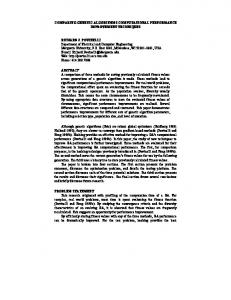
To better understand the behavior of the Hadoop implementation of cGA, we repeated the two experiment sets done in the case of the Hadoop SGA implementation. For each experiment, the population for the cGA is set to n log n where n is the number of variables. As done previously, 5 6

http://hadoop.apache.org http://cloud.cs.illinois.edu

10

10000 Time per iteration (in seconds)

140

Number of set bits

8000

6000

4000

2000

120 100 80 60 40 20

0

0 0

50

100

150 200 250 Number of Iterations

300

350

0

100 150 200 Number of Mappers

250

300

(b) Scalability of GA with constant load per node.

400

350

350

300 Time per iteration (in seconds)

Time per iteration (in seconds)

(a) Convergence of GA for 104 variables.

50

300 250 200 150 100

250 200 150 100 50

50 0 0

50

100 150 200 Number of Mappers

250

0 0 10

300

(c) Scalability of GA for 50, 000 variables with increasing number of mappers

10

1

10

2

3

10 10 Number of variables

4

10

5

10

6

(d) Scalability of GA with increasing number of variables.

Figure 2: Results obtained using Hadoop when implementing a simple genetic algorithm for solving the OneMAX problem.

11

200

140 80

●

●

40

60

●

●

●

150 100

● ●

●

●

●

● ●

●

● ●

●

50

100

Time per iteration (seconds)

●

0

0

20

Time per iteration (seconds)

120

● ●

0

50

100

150

200

250

300

1e+01

Number of mappers

(a) Scalability of compact genetic algorithm with constant load per node for the OneMAX problem.

1e+03

1e+05

1e+07

1e+09

Number of variables

(b) Scalability of compact genetic algorithm for OneMAX problem with increasing number of variables.

Figure 3: Results obtained using Hadoop when implementing the compact genetic algorithm. first we keep the load set to 200,000 variables per mapper. As shown in Figure 3(a), the time per iteration increases initially and then stabililizes around 75 seconds. Thus, increasing the problem size as more resources are added does not change the iteration time. Since, each node can run a maximum of 5 mappers, the overall map capacity is 5 · 52(nodes) = 260. Hence, around 250 mappers, the time per iteration increases due to the fact that no available resources (mapper slots) in the Hadoop framework are available. Thus, the execution must wait till mapper slots are released and the remaining portions can be executed, and the whole execution completed. In the second set of experiments, we utilized the maximum resources and increase the number of variables. As shown in Figure 3(b), our implementation scales to n = 108 variables, keeping the population set to n log n.

6

Discussion of Related Work

Several different models like fine grained (Maruyama et al., 1993), coarse grained (Lin et al., 1994) and distributed models (Lim et al., 2007) have been proposed for implementing parallel GAs. Traditionally, Message Passing Interface (MPI) has been used for implementing parallel GAs. However, MPIs do not scale well on commodity clusters where failure is the norm, not the exception. Generally, if a node in an MPI cluster fails, the whole program is restarted. In a large cluster, a machine is likely to fail during the execution of a long running program, and hence efficient fault tolerance is necessary. This forces the user to handle failures by using complex checkpointing techniques. MapReduce (Dean and Ghemawat, 2008) is a programming model that enables the users to easily develop large-scale distributed applications. Hadoop is an open source implementation of the MapReduce model. Several different implementations of MapReduce have been developed for other architectures like Phoenix (Raghuraman et al., 2007) for multicores and CGL12

MapReduce (Ekanayake et al., 2008) for streaming applications. To the best of our knowledge, MRPGA (Jin et al., 2008) is the only attempt at combining MapReduce and GAs. However, they claim that GAs cannot be directly expressed by MapReduce, extend the model to MapReduceReduce and offer their own implementation. We point out several shortcomings: Firstly, the Map function performs the fitness evaluation and the “ReduceReduce” does the local and global selection. However, the bulk of the work - mutation, crossover, evaluation of the convergence criteria and scheduling is carried out by a single co-ordinator. As shown by their results, this approach does not scale above 32 nodes due to the inherent serial component. Secondly, the “extension” that they propose can readily be implemented within the traditional MapReduce model. The local reduce is equivalent to and can be implemented within a Combiner (Dean and Ghemawat, 2008). Finally, in their mapper, reducer and final reducer functions, they emit “def ault key” and 1 as their values. Thus, they do not use any characteristic of the MapReduce model - the grouping by keys or the shuffling. The Mappers and Reducers might as well be independently executing processes only communicating with the co-ordinator. We take a different approach, trying to hammer the GAs to fit into the MapReduce model, rather than change the MapReduce model itself. We implement GAs in Hadoop, which is increasingly becoming the de-facto standard MapReduce implementation and used in several production environments in the industry. Meandre(Llor`a et al., 2008; Llor`a, 2009) extends beyond some limitations of the MapReduce model while maintaining a data-intensive nature. It shows linear scalability of simple GAs and EDAs on multicore architectures. For very large problems (> 109 variables), other models like compact genetic algorithms(cGA) and Extended cGA(eCGA) have been explored(Sastry et al., 2007).

7

Conclusions and Future Work

In this paper, we have mainly addressed the challenge of using the MapReduce model to scale simple and compact genetic algorithms. We described the algorithm design and implementation of GAs on Hadoop. The convergence and scalability of the implementation has been investigated. Adding more resources would enable us to solve even larger problems without any changes in the algorithm implementation. MapReducing more scalable GA models like extended compact GAs (Harik, 1999) will be investigated in future. We also plan to compare the performance with existing MPI-based implementations. General Purpose GPUs are an exciting addition to the heterogenity of clusters. The compute intensive Map phase and the random number generation can be scheduled on the GPUs, which can be performed in parallel with the Reduce on the CPUs. We would also like to demonstrate the importance of scalable GAs in practical applications.

Acknowledgment We would like to thank the anonymous reviewers for their valuable feedback. This research was funded, in part, by NSF IIS Grant #0841765. The views expressed are those of the authors only.

13

References Baluja, S. (1994). Population-based incremental learning: A method of integrating genetic search based function optimization and competitive learning. Technical Report CMU-CS-94163, Carnegie Mellon University. Baluja, S. and Caruana, R. (1995). Removing the genetics from the standard genetic algorithm. Technical Report CMU-CS-95-141, Carnegie Mellon University. Beynon, M. D., Kurc, T., Sussman, A., and Saltz, J. (2000). Design of a framework for dataintensive wide-area applications. In HCW ’00: Proceedings of the 9th Heterogeneous Computing Workshop, page 116, Washington, DC, USA. IEEE Computer Society. Cant´ u-Paz, E. (2000). Efficient and Accurate Parallel Genetic Algorithms. Springer. Dean, J. and Ghemawat, S. (2008). Mapreduce: Simplified data processing on large clusters. Commun. ACM, 51(1):107–113. Ekanayake, J., Pallickara, S., and Fox, G. (2008). Mapreduce for data intensive scientific analyses. In ESCIENCE ’08: Proceedings of the 2008 Fourth IEEE International Conference on eScience, pages 277–284, Washington, DC, USA. IEEE Computer Society. Foster, I. (2003). The virtual data grid: A new model and architecture for data-intensive collaboration. In in the 15th International Conference on Scientific and Statistical Database Management, pages 11–. Frnti, P., Kivijrvi, J., Kaukoranta, T., and Nevalainen, O. (1997). Genetic algorithms for large scale clustering problems. Comput. J, 40:547–554. Gallagher, K. and Sambridge, M. (1994). Genetic algorithms: a powerful tool for large-scale nonlinear optimization problems. Comput. Geosci., 20(7-8):1229–1236. Ghemawat, S., Gobioff, H., and Leung, S.-T. (2003). The google file system. SIGOPS Oper. Syst. Rev., 37(5):29–43. Goldberg, D., Deb, K., and Korb, B. (1989a). Messy genetic algorithms: motivation, analysis, and first results. Complex Systems, (3):493–530. Goldberg, D. E. (1989). Genetic algorithms in search, optimization, and machine learning. AddisonWesley, Reading, MA. Goldberg, D. E. (2002). The Design of Innovation: Lessons from and for Competent Genetic Algorithms. Kluwer Academic Publishers, Norwell, MA. Goldberg, D. E., Korb, B., and Deb, K. (1989b). Messy genetic algorithms: Motivation, analysis, and first results. Complex Systems, 3(5):493–530. Harik, G. (1999). Linkage learning via probabilistic modeling in the ecga. Technical report, University of Illinois at Urbana-Champaign). Harik, G., Cant´ u-Paz, E., Goldberg, D. E., and Miller, B. L. (1999). The gambler’s ruin problem, genetic algorithms, and the sizing of populations. Evolutionary Computation, 7(3):231–253. (Also IlliGAL Report No. 96004). 14

Harik, G., Lobo, F., and Goldberg, D. E. (1998). The compact genetic algorithm. Proceedings of the IEEE International Conference on Evolutionary Computation, pages 523–528. (Also IlliGAL Report No. 97006). Jin, C., Vecchiola, C., and Buyya, R. (2008). Mrpga: An extension of mapreduce for parallelizing genetic algorithms. eScience, 2008. eScience ’08. IEEE Fourth International Conference on, pages 214–221. Jong, K. D. and Sarma, J. (1995). On decentralizing selection algorithms. In In Proceedings of the Sixth International Conference on Genetic Algorithms, pages 17–23. Morgan Kaufmann. Larra˜ naga, P. and Lozano, J. A., editors (2002). Estimation of Distribution Algorithms. Kluwer Academic Publishers, Boston, MA. Lim, D., Ong, Y.-S., Jin, Y., Sendhoff, B., and Lee, B.-S. (2007). Efficient hierarchical parallel genetic algorithms using grid computing. Future Gener. Comput. Syst., 23(4):658–670. Lin, S.-C., Punch, W. F., and Goodman, E. D. (1994). Coarse-grain parallel genetic algorithms: Categorization and new approach. In Proceeedings of the Sixth IEEE Symposium on Parallel and Distributed Processing, pages 28–37. Llor`a, X. (2009). Data-intensive computing for competent genetic algorithms: a pilot study using meandre. In GECCO ’09: Proceedings of the 11th Annual conference on Genetic and evolutionary computation, pages 1387–1394, New York, NY, USA. ACM. ´ Llor`a, X., Acs, B., Auvil, L., Capitanu, B., Welge, M., and Goldberg, D. E. (2008). Meandre: Semantic-driven data-intensive flows in the clouds. In Proceedings of the 4th IEEE International Conference on e-Science, pages 238–245. IEEE press. Maruyama, T., Hirose, T., and Konagaya, A. (1993). A fine-grained parallel genetic algorithm for distributed parallel systems. In Proceedings of the 5th International Conference on Genetic Algorithms, pages 184–190, San Francisco, CA, USA. Morgan Kaufmann Publishers Inc. Mattmann, C. A., Crichton, D. J., Medvidovic, N., and Hughes, S. (2006). A software architecturebased framework for highly distributed and data intensive scientific applications. In ICSE ’06: Proceedings of the 28th international conference on Software engineering, pages 721–730, New York, NY, USA. ACM. M¨ uhlenbein, H. (1997). The equation for response to selection and its use for prediction. Evolutionary Computation, 5(3):303–346. M¨ uhlenbein, H. and Paaß, G. (1996). From recombination of genes to the estimation of distributions I. Binary parameters. Parallel Problem Solving from Nature, PPSN IV, pages 178–187. Pelikan, M., Lobo, F., and Goldberg, D. E. (2002). A survey of optimization by building and using probabilistic models. Computational Optimization and Applications, 21:5–20. (Also IlliGAL Report No. 99018). Raghuraman, R., Penmetsa, A., Bradski, G., and Kozyrakis, C. (2007). Evaluating mapreduce for multi-core and multiprocessor systems. Proceedings of the 2007 IEEE 13th International Symposium on High Performance Computer Architecture.

15

Sannomiya, N., Iima, H., Ashizawa, K., and Kobayashi, Y. (1999). Application of genetic algorithm to a large-scale scheduling problem for a metal mold assembly process. Proceedings of the 38th IEEE Conference on Decision and Control, 3:2288–2293. Sarma, A. J., Sarma, J., and Jong, K. D. (1998). Selection pressure and performance in spatially distributed evolutionary. In In Proceedings of the World Congress on Computatinal Intelligence, pages 553–557. IEEE Press. Sastry, K., Goldberg, D. E., and Llora, X. (2007). Towards billion-bit optimization via a parallel estimation of distribution algorithm. In GECCO ’07: Proceedings of the 9th annual conference on Genetic and evolutionary computation, pages 577–584, New York, NY, USA. ACM. Schaffer, J. and Eshelman, L. (1991). On Crossover as an Evolutionary Viable Strategy. In Belew, R. and Booker, L., editors, Proceedings of the 4th International Conference on Genetic Algorithms, pages 61–68. Morgan Kaufmann. Sywerda, G. (1989). Uniform crossover in genetic algorithms. In Proceedings of the third international conference on Genetic algorithms, pages 2–9, San Francisco, CA, USA. Morgan Kaufmann Publishers Inc. Uysal, M., Kurc, T. M., Sussman, A., and Saltz, J. (1998). A performance prediction framework for data intensive applications on large scale parallel machines. In In Proceedings of the Fourth Workshop on Languages, Compilers and Run-time Systems for Scalable Computers, number 1511 in Lecture Notes in Computer Science, pages 243–258. Springer-Verlag.

16