Apr 30, 2008 - functions, fA(x0), fP(x0) in the pseudoscalar channel, kV(x0) in the ..... [2] M. Lüscher, R. Narayanan, P. Weisz and U. Wolff, âThe Schrödinger functional: .... lattice QCD simulations and the thermodynamic limit,â JHEP 0602 ...
arXiv:0804.3383v2 [hep-lat] 30 Apr 2008
CERN-PH-TH-2008-079 DESY 08-043 HU-EP-08/12 MIT-CTP 3942 MS-TP-08-5 SFB/CPP-08-22
Scaling test of two-flavor O(a)–improved lattice QCD
ALPHA Collaboration
Michele Della Mortea,f , Patrick Fritzschb , Harvey Meyerc,e , Hubert Simmad,e , Rainer Sommere , Shinji Takedaf , Oliver Witzelf , Ulli Wolfff a
CERN, Physics Department, TH Unit, CH-1211 Geneva 23, Switzerland Institut f¨ ur Theoretische Physik, Westf¨ alische Wilhelms-Universit¨ at M¨ unster, Wilhelm-Klemm-Strasse 9, D-48149 M¨ unster, Germany c Center for Theoretical Physics, Massachusetts Institute of Technology, Cambridge, MA 02139, USA d Universit` a di Milano Bicocca, Piazza della Scienza 3, 20126 Milano, Italy e DESY, Platanenallee 6, 15738 Zeuthen, Germany Institut f¨ ur Physik, Humboldt Universit¨ at, Newtonstr. 15, 12489 Berlin, Germany b
f
Abstract We report on a scaling test of several mesonic observables in the non-perturbatively O(a) improved Wilson theory with two flavors of dynamical quarks. The observables are constructed in a fixed volume of 2.4 fm × (1.8 fm)3 with Schr¨ odinger functional boundary conditions. No significant scaling violations are found. Using the kaon mass determined (2) in [1], we update our estimate of the Lambda parameter to ΛMS /mK = 0.52(6).
1
Introduction
In this article we summarize the results of a set of simulations of QCD with two degenerate flavors of quarks employing Schr¨ odinger functional boundary conditions [2]. The range of quark masses covered corresponds to a ratio of the pseudoscalar mass to the vector mass, MPS / MV , in the interval [0.4, 0.75]. Our final goal is to compute the fundamental parameters of perturbative QCD, namely the scale parameter Λ and the quark masses Mq , in units of a hadronic observable such as the Kaon decay constant FK . We emphasize our effort to control all systematics. Here we focus on cutoff effects and reach (for one quark mass) a lattice spacing that is smaller than those previously achieved in large-volume simulations of the O(a) improved Wilson action [1, 3, 4, 5]. While simulations of QCD with at least Nf = 2+1 flavors of sea quarks are mandatory to provide accurate non-perturbative predictions with direct phenomenological implications, in our view the Nf = 2 theory represents a framework well suited to address a number of fundamental aspects of low-energy QCD that have not been clarified yet, a couple of which we shall presently mention. One such question is the Nf dependence of ΛMS / FK and Ms / FK . Since these quantities have been computed in the quenched theory [6, 7], it is interesting to know the separate effects of the (up, down) quarks and those of the strange quark. To our knowledge, the influence of the strange sea quarks on hadronic observables has not been demonstrated very clearly so far. Secondly, it is important to determine the quark mass at which one-loop SU(2) chiral perturbation theory becomes accurate at the (say) 3% level. We see a strong motivation to address this question in the Nf = 2 theory, with one parameter less to tune on the QCD side. And with a small number of low-energy constants in the chiral perturbation theory, this is probably the cleanest way to establish the latter as the low-energy description of QCD from first principles. Given the level of accuracy one is interested in, all sources of systematic error have to be addressed. In particular any observed non2 must first be shown to survive linearity in the quark-mass dependence of FPS and MPS the infinite volume limit before it can be claimed that the chiral logarithms have been observed. Cutoff effects represent an additional source of systematic uncertainty, which is computationally expensive to reduce. In particular, cutoff effects may be larger in the presence of sea-quarks [8]. With Wilson fermions, even in their O(a) improved version that we employ, it is well known that the chiral limit does not commute with the continuum limit, implying that at fixed lattice spacing a cutoff effects become large below some quark mass. It is therefore important to control cutoff effects as one proceeds to simulate deeper in the chiral regime. In the quenched work [9], rather accurate results were obtained in the pseudoscalar and vector channels using the Schr¨ odinger functional. In this paper we carry over this computational setup to the Nf = 2 theory. The accuracy achieved [9] on masses was comparable to the calculations performed with periodic boundary conditions, and for decay constants the Schr¨ odinger functional even proved to be the superior method. This is different when dynamical fermions are present. As shown in [10] multi-pion excited states contribute significantly. For a computation of ground state masses and matrix elements they have to be supressed by a rather large time extent of the Schr¨ odinger functional – in particular when the quark mass is low. In this situation it is more 1
practical to employ (anti)periodic boundary conditions with the associated translation invariance in time. We can nonetheless use our simulation results to perform a first scaling test of the Nf = 2 O(a)-improved theory at low energies. Note that at high energies and correspondingly small lattice spacings excellent scaling has been seen [11, 12]. Besides the scaling test we give some details of our simulations including the algorithmic performance (section 2).
2
Lattice simulations
Our discretization consists of the Wilson gauge action and the non-perturbatively O(a) improved Wilson quark action, with csw given in [13]. The algorithm and solver used in the present simulations have been described in some detail in [14, 15]. Using the notation of [16] for the hopping terms of the Dirac operator1 , we recall the Schur complements of the hermitian Dirac operator with respect to asymmetric and symmetric even-odd ˆ A, Q ˆ preconditioning Q ˆ A = cˆ γ5 (Moo − Moe M −1 Meo ) , Q ee
ˆ = M −1 Q ˆA , Q oo
cˆ = (1 + 64κ2 )−1 .
(1)
The action then reads S = SG + Spf + Sdet ,
(2)
with Spf
h
−2 ˆQ ˆ † + ρ20 Moo = φ†0 Q
i−1
h
i
ˆ −2 φ0 + φ†1 ρ−2 0 + QA φ1
Sdet = (−2) log det Mee + (−2) log det Moo ,
(3) (4)
and SG is the plaquette action. The determinants appearing in Sdet are taken into account exactly. In Tab. 1 and Tab. 2 we list the simulations discussed in this paper. The reference length scale L∗ is defined through g¯2 (L∗ ) = 5.5, where g¯ is the Schr¨ odinger functional coupling, and the values it assumes at the relevant bare couplings were presented in [10]. For an estimate of L∗ in fermis, one may use the result a = 0.0784(10)fm at β = 5.3 [1], yielding L∗ ≈ 0.6fm. Renormalization is carried out non-perturbatively in the SF at the scale µren = 1/Lren , where g¯2 (Lren ) = 4.61. The values of the renormalization factor ZP of the pseudoscalar density are taken from [17], while the values of the renormalization factor ZA of the axial current differ from [17]. They are presently re-evaluated using a Ward identity in a 1.8 fm × (1.2 fm)3 Schr¨ odinger functional where the O(a2 ) effects are significantly smaller than before. In the table we list our preliminary numbers [18], which are not expected to change by more than the quoted errors.
2.1
Stability and the spectral gap
The spectral gap µ of the Hermitian Dirac operator was used in [19] as a tool to diagnose the stability of the HMC algorithm. We define n√ o 1 ˆQ ˆ† , min λ λ is an eigenvalue of Q (5) µ ˆ= 4κˆ c 1
Moo , Mee correspond to 1 + Too and 1 + Tee respectively in [16, 15].
2
(L/a)3 × T /a
κ
L∗ /a
ZA
ZP
5.5
32 × 42
0.13630
10.68(15)
0.805(5)
0.5008(70)
5.3
243 × 32
0.13550 0.13590 0.13605 0.13625
7.82(6)
0.781(8)
0.4939(34)
5.2
163 × 32 243 × 32
0.13568 0.13568
6.51(12)
0.769(12)
0.4788(5)
sim. A1 B1 , B1′ B2 B3 B4 C1 C2
β
3
Table 1: Simulation parameters. We use L∗ , defined by g¯2 (L∗ ) = 5.5, as a reference scale. The renormalization factor of the axial current [17, 18], ZA , and of the pseudoscalar density [11] at scale µren are listed.
(0)
A1 B1 B1′ B2 B3 B4 C1 C2
mol. dyn. Nrep · τtot ρ0 hNCG i [LF; 2; 5; 50] 1 · 4340 0.019803 170 [SW; 2; 1; 64] 2 · 2400 0.0300 100 0.0300 100 [SW; 12 ; 1; 16] 2 · 1750 [SW; 21 ; 1; 16] 2 · 1900 0.0300 102 [LF; 2; 5; 50] 2 · 2600 0.019803 143 [LF; 2; 5; 50] 2 · 1448 0.0180 155 [LF; 2; 5; 64] 1 · 6500 0.0198 179 [LF; 2; 5; 80] 2 · 2080 0.0198 184
(1)
hNCG i 824 482 485 729 905 1195 791 1086
Pacc 88% 91% 90% 90% 91% 87% 96% 94%
Table 2: Algorithmic parameters of the simulations. The molecular dynamics is characterized by [Integrator; τ ; δτ1 /δτ0 ; τ /δτ1 ], where the integrator can be ‘leap-frog’ or ‘Sexton-Weingarten’ and subscripts refer to the two pseudofermions in use. For the (k) gauge force, the SW integrator with δτ0 /δτg = 4 is used in all cases, and hNCG i is the number of conjugate-gradient iterations used to solve the symmetrically even-odd preconditioned Dirac equation during the trajectory.
3
200 L=16 L=24
v
N( a µ )
150
100
50
0 0
0.005
0.01
0.015
0.02
0.025
0.03
v
aµ
Figure 1: Histogram of µ ˆ for two different spatial volumes, simulations C1 and C2 . The median is indicated in each case by the vertical dashed line. normalized such that it is given by the quark mass in the free theory with periodic boundary conditions. Since the only term that can potentially lead to unbounded flucˆ a sufficient condition tuations of the molecular dynamics forces is associated with Q, for the stability of the algorithm is for the distribution of µ ˆ to be well separated from the origin. We remark that µ ˆ and µ (which was considered in [19]) cannot be directly compared on a quantitative level as they differ by the boundary conditions in the time direction and due to our (symmetric) even-odd preconditioning. We obtained µ ˆ by comˆQ ˆ † using the algorithm of [20]. Figure 1 displays the puting the lowest eigenvalue of Q histogram of µ ˆ for simulations C1,2 . There is a clear separation of the median of the distribution from the origin, but in a few cases in the course of the simulations eigenvalues as small as a third of this value were seen. We consider now the variance σ ˆ 2 of µ ˆ. In [19],pa measure σ of the width of the µ distribution was found to approximately satisfy aσ L3 T /a4 ≈ constant. In the subset of our simulations where we computed µ ˆ, we find σ ˆ
√
L3 T /a
=
1.437(64)
1.268(23)
1.477(33)
varying only by about 15%.
4
A1 C1 C2 ,
(6)
2.2
Autocorrelation times
We compile observed integrated autocorrelation times τint [22] in Tab. 3 for five quantities discussed and defined in detail in the next section. The dependence of the autocorrelation times on the trajectory length was discussed previously [23]. Here we note that while there is a tendency for the autocorrelation time of the plaquette to decrease when the lattice spacing is increased, for other observables the opposite trend appears to be present underlining that autocorrelations have to be monitored for each observable separately. The most important information in Tab. 3 is that all autocorrelations are small compared to the length of the runs (cf. Tab. 2). Error estimates are hence trustworthy. P V m(T /2) mA eff (T /2) meff (T /2) Feff (T /2) meff (T /2) Geff (T /2)
τint [O]
P
A1 B1 B1′ B2 B3 B4 C1 C2
5.0(9) 13(3) 6(1) 4.1(7) 9(2) 8(2) 9(2) 11(3)
4.9(9) 5.5(9) 6(1) 4.1(7) 3.9(6) 5(1) 5.3(8) 6(1)
11(3) 7(1) 10(2) 10(3) 4.7(7) 6(1) 5.2(8) 6(1)
21(6) 16(4) 22(7) 14(4) 11(2) 7(2) 5.1(8) 7(1)
10(2) 4.2(7) 14(4) 8(2) 6(1) 4.6(9) 4.7(7) 3.9(6)
40(10) 23(7) 24(8) 23(7) 11(3) 15(5) 4.9(7) 6(1)
23(7) 11(3) 12(3) 24(8) 11(2) 8(2) 5.6(9) 6(1)
Table 3: The integrated autocorrelation times for the plaquette, the current quark mass, the effective pseudoscalar mass and decay constant, and the effective vector mass. The unit is molecular dynamics time, i. e. trajectories times the length of the trajectory. For a precise definition of the observables see the following section.
3
Scaling test
In this section, which represents the central part of this paper, we investigate the cutoff effects on a number of non-perturbatively renormalized quantities. In order to keep systematic effects due to a varying volume negligible, we compare series of simulations in a fixed (but quite large) volume on a physical scale. More precisely we determine L/L∗ = 3.00(4), 3.07(3) and T /L∗ = 3.93(4), 4.09(3) on the A and B lattices. At β = 5.2, the volumes came out less uniform, L(C1 )/L∗ = 2.46(5), L(C2 )/L∗ = 3.69(6) and T (Ci )/L∗ = 4.92(10). We shall discuss how to correct for these small mismatches after introducing the finite volume observables of this study. They are extracted from the zero spatial momentum boundary-to-bulk correlation functions, fA (x0 ) , fP (x0 ) in the pseudoscalar channel, kV (x0 ) in the vector channel and the boundary-to-boundary pseudoscalar correlator f1 [9]. We include the O(a) improvement term proportional to cA [21] in fA,I = fA +a cA ∂0 fP . Effective masses and decay constants 1 ∗ mA eff (x0 ) ≡ − 2 (∂0 + ∂0 ) log(fA,I (x0 )) 1 ∗ mP eff (x0 ) ≡ − 2 (∂0 + ∂0 ) log(fP (x0 ))
mV eff (x0 )
≡
− 21 (∂0∗
+ ∂0 ) log(kV (x0 )) 5
(7) (8) (9)
sim.
am
a mA eff
a mP eff
a mV eff
a Feff ZA (1+bA a mq )
a2 Geff ZP (1+bp a mq )
A1 B1 B2 B3 B4 C1 C2 CI
0.015519(37) 0.03388(12) 0.019599(95) 0.01460(11) 0.00727(14) 0.01401(21) 0.01442(14) 0.01431(19)
0.1800(20) 0.3272(18) 0.2391(35) 0.2118(24) 0.1423(55) 0.2173(55) 0.2328(39) 0.2286(97)
0.1793(15) 0.3236(16) 0.2406(19) 0.2066(17) 0.1528(20) 0.2338(24) 0.2261(15) 0.2282(63)
0.2821(50) 0.4520(35) 0.3953(51) 0.3647(35) 0.3058(69) 0.4354(60) 0.4152(42) 0.410(14)
0.05999(42) 0.09451(41) 0.08442(68) 0.07714(60) 0.0698(11) 0.0877(13) 0.08773(67) 0.08772(61)
0.0629(10) 0.1507(14) 0.1267(22) 0.1170(13) 0.0985(15) 0.1637(25) 0.1614(15) 0.1620(17)
Table 4: Simulation results for the effective quantities evaluated at x0 = T /2. The bare current quark mass has been averaged over T /3 ≤ x0 ≤ 2T /3. The last line gives the interpolation of C1 , C2 , including the corrections described in the text.
Feff (x0 ) ≡ −2ZA
fA (x0 ) (1 + bA a mq ) exp(mA eff (x0 )(x0 − T /2)) �1/2
= −2ZA (1 + bA a mq ) Geff (x0 ) ≡ 2ZP (1 + bp a mq ) = 2ZP (1 + bp a mq )
3 f 1 mA eff (x0 ) L fA,I (T /2)
3 f 1 mA eff (T /2) L
�1/2
at x0 = T /2
(10)
P 1/2 fP (x0 ) exp(mP eff (x0 )(x0 − T /2)) meff (x0 )
(f1 L3 )1/2
1/2 fP (T /2) mP eff (T /2)
(f1 L3 )1/2
at
x0 = T /2
(11)
are related to (L-dependent) masses and matrix elements, P mA eff (x0 ) ≈ MPS ≈ meff (x0 ) ,
mV eff (x0 ) ≈ MV ,
Feff (x0 ) ≈ FPS ,
Geff (x0 ) ≈ GPS .(12)
These relations hold in the limit of large x0 and T up to correction terms [9] Oeff (x0 ) = O + ηO exp(−(E1 − MPS ) x0 ) + η˜O exp(−E2 (T − x0 )) + . . . ,
(13)
where the coefficients ηO and η˜O are ratios of matrix elements, E1 is the energy of the first excitation in the zero momentum pion channel and E2 in the vacuum channel. For not too small L and not too large MPS we expect E1 ≈ 3 MPS and E2 ≈ 2 MPS . Our results for the effective observables at x0 = T /2 are listed in Tab. 4 together with the bare current quark mass m stabilized by averaging over T /3 ≤ x0 ≤ 2T /3, m =
n2 X 1 m(x0 ) , n2 − n1 + 1 x /a=n 0
m(x0 ) =
1 ∗ 2 (∂0
1
n1 ≥ T /3a , n2 ≤ 2T /3a
+ ∂0 )fA (x0 ) + cA a∂0∗ ∂0 fP (x0 ) . 2fP (x0 )
(14) (15)
The results at β = 5.3 can be compared directly to those of [3], shown in Tab. 5, for which the correction terms in Eq. (13) can safely be neglected. In other words they 6
sim.
am
a MPS
a MV
a FPS ZA (1+bA a mq )
a2 GPS ZP (1+bp a mq )
D1 D2 D4
0.03386(11) 0.01957(07) 0.00761(07)
0.3286(10) 0.2461(09) 0.1499(15)
0.464(3) 0.401(3) 0.344(9)
0.0949(13) 0.0815(10) 0.0689(13)
0.1512(20) 0.1260(16) 0.1017(24)
Table 5: Observables from fits of [3] i.e. x0 , T → ∞. Input parameters β, κ and L/a match those of lattices B1 , B2 , B4 ; note that D4 has been renamed here compared to [3].
correspond to x0 , T → ∞. This allows us to estimate the effects due to T (C) > T (A) ≈ T (B) in addition to those coming from the mismatch in L. 1. For the matrix elements Feff , Geff no systematic differences between B and D lattices are visible. No correction due to T is necessary. We just interpolate the C1 and C2 results in L to L/L∗ = 3 using the Ansatz a1 + a2 L−3/2 e− MPS L , with MPS the pion mass on the larger volume. A small systematic error is added linearly to the statistical one. It is estimated by comparing with the result from an alternative interpolation with a′1 + a′2 L−1 . P 2. We observe | mP eff (B)/ meff (D)−1| ≤ 0.03 without a systematic trend as a function of the quark mass. We take this into account as a systematic error of 2% on mP eff (C) and2 subsequently we interpolate in L as in 1. The numbers for mA are not used eff further. V 3. Finite T effects are not negligible in the vector mass (mV eff (B)/ meff (D) − 1 ≈ −0.10 . . . − 0.03). We thus first perform a correction for the finite T effects using fits to Eq. (13) with E1 = 2(MPS 2 +(2π/L)2 )1/2 , E2 = 2 MPS . A systematic error of 50% of this correction is included for the result. Next the finite L correction is performed as above.
The interpolated values are included in Tab. 4 as “simulation” CI . After these small corrections we are ready to look at the lattice spacing dependence of our observables. To this end the necessary renormalization factors are attached (with perturbative values for bA , bp [24]) and we form dimensionless combinations by multiplying with L∗ . At 2 ∝ m. It lowest order in the quark mass expansion (in large volume), one has MPS P ∗ 2 ∗ is thus natural to consider [meff L ] /[m(µ ¯ ren )L ] instead of the quark mass itself. We choose m ¯ renormalized non-perturbatively in the SF scheme at scale µren = 1/Lren where g¯2 (Lren ) = 4.61 [11]. The quantities considered are shown in Fig. 2 as a function of the ∗ 2 dimensionless [mP eff L ] . At β = 5.3 we have a few quark-mass points. As a reference, ∗ 2 these are locally interpolated in [mP eff L ] with a second order polynomial. For masses lighter than in simulation B2 , the interpolation involves the lightest three masses and for heavier ones, it involves the heaviest three masses. The two-sigma bands (±2σ) of these interpolations are depicted as dotted vertical lines. Our results at the other β-values are seen to be in agreement with these error bands, which are generally around 5%, but 2
From Eq. (13) this finite T effect scales with exp(− MPS T ), yielding a reduction of 3% by a factor [1 − exp(− MPS L∗ )] when one considers the difference between T ≈ 5L∗ and the target T = 4L∗ .
7
5
β=5.2 β=5.3 β=5.5
4.5
4
3.5
3
2.5
2
1.5
1
0.5 0
1
2
3
4
P [meff (T/2)
5
6
7
*2
L]
Figure 2: Dimensionless renormalized finite volume observables as a function of ∗ 2 ∗ 2 V ∗ ∗ P ∗ 2 ¯ ∗ [mP ren )L ]/15 eff L ] . From top to bottom Geff (L ) , meff L , 4 Feff L , [meff L ] /[m(µ are shown. Squares, circles and triangle are for β = 5.2 , 5.3 , 5.5 respectively. Effective quantities are at x0 = T /2. The dotted band is an interpolation of the β = 5.3 data as described in the text.
8
2.8 B 2 fA 2.6
B 2 fP A1 fA
2.4
A1 fP
meff( x0 ) L
*
2.2 2 1.8 1.6 1.4 1.2 1 0.8 0
0.5
1
1.5 x0 / L
2 -2
*
-1.5
-1 * - (T-x0) / L
-0.5
0
P Figure 3: The effective pseudoscalar masses mA eff and meff in simulations B2 and A1 . The horizontal error bars are shown on some of the points only for clarity. The horizontal line is to guide the eye. The vertical line indicates the middle of the B2 lattice. ∗ 2 ¯ ∗ 10% for [mP ren )L ] after all errors are included. Even if the precision is not eff L ] /[m(µ very impressive, large cutoff effects are clearly absent. So far we have discussed the scaling of the ground state properties for a given symmetry channel. We now turn to the size of cutoff effects affecting excited state contributions P to the correlators. Figure 3 compares the effective pseudoscalar masses mA eff and meff in simulation A1 and B2 . The large size of the excited state contributions [10], while a drawback in extracting ground state properties, means that these functions are rather sensitive to the aforementioned cutoff effects. Because the A1 time extent is shorter by 4(1)%, on this figure we have separately aligned the two boundaries of lattice A1 and B2 . We observe that the two data sets are consistent within uncertainties well before the function flattens off. With the exception of mP eff for x0 < T /2, the agreement sets in at a distance to the closest boundary of about L∗ , where it is easily seen that several excited states contribute significantly to the correlation functions. Altogether this figure is evidence that the masses and matrix elements of the first excited state in both the pion and vacuum channel have scaling violations not exceeding the few percent level. But higher states can have rather significant discretization errors.
4
(2)
Conclusion and an updated value of ΛMS
We carried out a finite size scaling test of the standard non-perturbatively O(a)-improved [25, 26, 13] Wilson theory with two flavors of dynamical fermions. In contrast to previous 9
indications [8], cutoff effects are rather small in the present situation where the linear extent of the volume is around 1.6 fm. In fact within our precision of about 5% (collecting all errors) for effective masses and matrix elements, no a2 effects are visible. Continuum extrapolations of data from (say) 0.08 fm ≤ a ≤ 0.04 fm lattices which can nowadays be simulated [27, 28], seem very promising. Such a programme has been initiated [29]. A complementary effort [30] uses the twisted mass regularization of QCD [31]. Also in this case linear a-effects are absent [32] and the O(a2 ) effects appear to be moderate [33]. Finally we exploit the increased confidence in the scaling behavior of the simulated lattice theory to slightly refine our earlier estimate of the Λ-parameter. In [12] the product L∗ ΛMS = 0.801(56) was computed non-perturbatively in the two-flavor theory. (2)
Setting the scale through r0 = 0.5 fm the value ΛMS = 245(16)(16) MeV was obtained emphasizing that more physical observables should be used in the future to set the scale. Given the quality of scaling observed in the previous section, it seems safe to assume that L∗ mK in the continuum limit differs by no more than 5% from its value at β = 5.3 where mK a = 0.197(10) from [1, 3] and L∗ /a = 7.82(6) [10] are known.3 We then obtain (2) (2) ΛMS /mK = 0.52(6) or ΛMS = 257(26) MeV, where a 5% uncertainty for a possible scaling violation has been added to the error (in quadrature). The new estimate is a bit higher than the previous one [12].
Acknowledgements We thank DESY/NIC for computing resources on the APE machines and the computer team for support, in particular to run on the apeNEXT systems. This project is part of ongoing algorithmic development within the SFB Transregio 9 “Computational Particle Physics” programme. We thank the authors of [1] for discussions and for communicating simulation results prior to publication.
References [1] L. Del Debbio, L. Giusti, M. L¨ uscher, R. Petronzio and N. Tantalo, “QCD with light Wilson quarks on fine lattices. I: First experiences and physics results,” JHEP 0702 (2007) 056 [arXiv:hep-lat/0610059]. [2] M. L¨ uscher, R. Narayanan, P. Weisz and U. Wolff, “The Schr¨ odinger functional: A Renormalizable probe for nonAbelian gauge theories,” Nucl. Phys. B 384, 168 (1992) [arXiv:hep-lat/9207009]; S. Sint, “On the Schr¨ odinger functional in QCD,” Nucl. Phys. B 421, 135 (1994) [arXiv:hep-lat/9312079]; S. Sint, “One Loop Renormalization Of The QCD Schr¨ odinger Functional,” Nucl. Phys. B 451, 416 (1995) [arXiv:hep-lat/9504005]. [3] L. Del Debbio, L. Giusti, M. L¨ uscher, R. Petronzio and N. Tantalo, “QCD with light Wilson quarks on fine lattices. II: DD-HMC simulations and data analysis,” JHEP 0702 (2007) 082 [arXiv:hep-lat/0701009]. 3
We have used mK = mK,ref with an error of 5% where mK,ref is defined in [1].
10
[4] D. Brommel et al. [QCDSF/UKQCD Collaboration], “The pion form factor from lattice QCD with two dynamical flavours,” Eur. Phys. J. C 51 (2007) 335 [arXiv:hep-lat/0608021]. [5] S. Aoki et al. [JLQCD Collaboration], “Light hadron spectroscopy with two flavors of O(a)-improved dynamical Phys. Rev. D 68 (2003) 054502 [arXiv:hep-lat/0212039]. [6] S. Capitani, M. L¨ uscher, R. Sommer and H. Wittig [ALPHA Collaboration], “Nonperturbative quark mass renormalization in quenched lattice QCD,” Nucl. Phys. B 544, 669 (1999) [arXiv:hep-lat/9810063]. [7] J. Garden, J. Heitger, R. Sommer and H. Wittig [ALPHA Collaboration], “Precision computation of the strange quark’s mass in quenched QCD,” Nucl. Phys. B 571, 237 (2000) [arXiv:hep-lat/9906013]. [8] R. Sommer et al. [ALPHA Collaboration], “Large cutoff effects of dynamical Wilson fermions,” Nucl. Phys. Proc. Suppl. 129 (2004) 405 [arXiv:hep-lat/0309171]. [9] M. Guagnelli, J. Heitger, R. Sommer and H. Wittig [ALPHA Collaboration], “Hadron masses and matrix elements from the QCD Schr¨ odinger functional,” Nucl. Phys. B 560 (1999) 465 [arXiv:hep-lat/9903040]. [10] M. Della Morte et al., “Preparing for Nf =2 simulations at small lattice spacings,” PoS LAT2007 (2007) 255 [arXiv:0710.1263 [hep-lat]]. [11] M. Della Morte, R. Hoffmann, F. Knechtli, J. Rolf, R. Sommer, I. Wetzorke and U. Wolff [ALPHA Collaboration], “Non-perturbative quark mass renormalization in two-flavor QCD,” Nucl. Phys. B 729 (2005) 117 [arXiv:hep-lat/0507035]. [12] M. Della Morte, R. Frezzotti, J. Heitger, J. Rolf, R. Sommer and U. Wolff [ALPHA Collaboration], “Computation of the strong coupling in QCD with two dynamical flavours,” Nucl. Phys. B 713 (2005) 378 [arXiv:hep-lat/0411025]. [13] K. Jansen and R. Sommer [ALPHA collaboration], “O(alpha) improvement of lattice QCD with two flavors of Wilson quarks,” Nucl. Phys. B 530 (1998) 185 [Erratum-ibid. B 643 (2002) 517] [arXiv:hep-lat/9803017]. [14] H. B. Meyer and O. Witzel, “Trajectory length and autocorrelation times: N(f) = 2 simulations in the Schr¨ odinger functional,” PoS LAT2006, 032 (2006) [arXiv:hep-lat/0609021]. [15] M. Della Morte, F. Knechtli, J. Rolf, R. Sommer, I. Wetzorke and U. Wolff [ALPHA Collaboration], “Simulating the Schr¨ odinger functional with two pseudo-fermions,” Comput. Phys. Commun. 156 (2003) 62 [arXiv:hep-lat/0307008]. [16] K. Jansen and C. Liu, “Implementation of Symanzik’s improvement program for simulations of dynamical Wilson fermions in lattice QCD,” Comput. Phys. Commun. 99 (1997) 221, [arXiv:hep-lat/9603008].
11
[17] M. Della Morte, R. Hoffmann, F. Knechtli, R. Sommer and U. Wolff, “Nonperturbative renormalization of the axial current with dynamical Wilson fermions,” JHEP 0507, 007 (2005) [arXiv:hep-lat/0505026]. [18] M. Della Morte, R. Sommer and S. Takeda, work in progress [19] L. Del Debbio, L. Giusti, M. L¨ uscher, R. Petronzio and N. Tantalo, “Stability of lattice QCD simulations and the thermodynamic limit,” JHEP 0602 (2006) 011 [arXiv:hep-lat/0512021]. [20] T. Kalkreuter and H. Simma, “An Accelerated Conjugate Gradient Algorithm To Compute Low Lying Comput. Phys. Commun. 93, 33 (1996) [arXiv:hep-lat/9507023]. [21] M. Della Morte, R. Hoffmann and R. Sommer, “Non-perturbative improvement of the axial current for dynamical Wilson fermions,” JHEP 0503, 029 (2005) [arXiv:hep-lat/0503003]. [22] U. Wolff [ALPHA collaboration], “Monte Carlo errors with less errors,” Comput. Phys. Commun. 156, 143 (2004) [Erratum-ibid. 176, 383 (2007)] [arXiv:hep-lat/0306017]. [23] H. B. Meyer, H. Simma, R. Sommer, M. Della Morte, O. Witzel and U. Wolff, “Exploring the HMC trajectory-length dependence of autocorrelation times in lattice QCD,” Comput. Phys. Commun. 176 (2007) 91 [arXiv:hep-lat/0606004]. [24] S. Sint and P. Weisz, “Further results on O(a) improved lattice QCD to one-loop order of perturbation theory,” Nucl. Phys. B 502 (1997) 251 [arXiv:hep-lat/9704001]. [25] B. Sheikholeslami and R. Wohlert, “Improved Continuum Limit Lattice Action For QCD With Wilson Fermions,” Nucl. Phys. B 259 (1985) 572. [26] M. L¨ uscher, S. Sint, R. Sommer and P. Weisz, “Chiral symmetry and O(a) improvement in lattice QCD,” Nucl. Phys. B 478 (1996) 365 [arXiv:hep-lat/9605038]. [27] M. L¨ uscher, “Schwarz-preconditioned HMC algorithm for two-flavour lattice QCD,” Comput. Phys. Commun. 165 (2005) 199 [arXiv:hep-lat/0409106]. [28] M. L¨ uscher, “Deflation acceleration of lattice QCD simulations,” JHEP 0712 (2007) 011 [arXiv:0710.5417 [hep-lat]]. [29] https://twiki.cern.ch/twiki/bin/view/CLS/WebHome [30] Ph. Boucaud et al. [ETM Collaboration], “Dynamical twisted mass fermions with light quarks,” Phys. Lett. B 650, 304 (2007) [arXiv:hep-lat/0701012]. [31] R. Frezzotti, P. A. Grassi, S. Sint and P. Weisz [Alpha collaboration], “Lattice QCD with a chirally twisted mass term,” JHEP 0108 (2001) 058 [arXiv:hep-lat/0101001]. [32] R. Frezzotti and G. C. Rossi, “Chirally improving Wilson fermions. I: O(a) improvement,” JHEP 0408 (2004) 007 [arXiv:hep-lat/0306014]. 12
[33] P. Dimopoulos, R. Frezzotti, G. Herdoiza, C. Urbach and U. Wenger [ETM Collaboration], “Scaling and low energy constants in lattice QCD with Nf =2 maximally PoS LAT2007 (2007) 102 [arXiv:0710.2498 [hep-lat]].
13