distortions, by rectifying the 3D point clouds from the range sensor. ... come
popular, e.g. Microsoft Kinect and the Asus WAVI ..... 200. 85. 86. 87. 88. 89. 90.
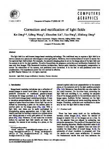
91. 1 − 2. 1 − 3. 2 − 3. Figure 5. Angles between box sides, as function of
rotational ve-.
Scan Rectification for Structured Light Range Sensors with Rolling Shutters Erik Ringaby and Per-Erik Forss´en Department of Electrical Engineering Link¨oping University, Sweden {ringaby,perfo}@isy.liu.se
Abstract Structured light range sensors, such as the Microsoft Kinect, have recently become popular as perception devices for computer vision and robotic systems. These sensors use CMOS imaging chips with electronic rolling shutters (ERS). When using such a sensor on a moving platform, both the image, and the depth map, will exhibit geometric distortions. We introduce an algorithm that can suppress such distortions, by rectifying the 3D point clouds from the range sensor. This is done by first estimating the time continuous 3D camera trajectory, and then transforming the 3D points to where they would have been, if the camera had been stationary. To ensure that image and range data are synchronous, the camera trajectory is computed from KLT tracks on the structured-light frames, after suppressing the structured-light pattern. We evaluate our rectification, by measuring angles between the visible sides of a cube, before and after rectification. We also measure how much better the 3D point clouds can be aligned after rectification. The obtained improvement is also related to the actual rotational velocity, measured using a MEMS gyroscope.
Figure 1. Top row: Depth map, and NIR frame from a Kinect sequence acquired during fast motion. Bottom row: Re-projected depth map, and NIR frame from rectified point cloud. The structured light pattern in the NIR frames have been suppressed using the method in section 3.
ever, the high price for time-of-flight and laser-range sensors have this far limited a more widespread use. SLRS are directly useful for short range obstacle perception (typically up to 3.5m [17]), and they also have the potential to be useful in simultaneous localisation and mapping (SLAM) [12]. Doing SLAM using these devices is somewhat problematic, as they make use of CMOS cameras with electronic rolling shutters (ERS). In an ERS camera, all pixels are not exposed at the same time (as is the case in a global shutter camera). Instead each row is exposed at a slightly different time interval, that is characterised by the sensor readout time [10, 9, 2]. The effect of this is geometric distortions in the image, when either the camera or the scene changes during exposure, see figure 1, top row. Unless rolling shutter distortions are modelled, a SLAM system using a rolling shutter sensor is limited to slow motions, or move-stop-look image acquisition cycles (analogous to stop motion animation). In this paper, we introduce an algorithm that rectifies
1. Introduction Structured light range sensors (SLRS) have recently become popular, e.g. Microsoft Kinect and the Asus WAVI Xtion. Both these devices are based on a patented reference implementation by the company Primesense [17]. The intended purpose for these sensors is full body gesture based human-computer interfaces. As these devices deliver quasidense depth maps at 30 fps (computed using a built-in SoC) they also have many other applications (see e.g. http://kinecthacks.net/ for some examples). We want to make these sensors more useful for dynamic robot perception. 3D range sensing has proven to be very useful for autonomous robots, as demonstrated in the 2007 DARPA urban challenge [21]. In this competition, all of the successful contenders made heavy use of 3D sensing, both for mapping, and to perceive nearby obstacles. How1
sensor data affected by rolling shutter distortions. An example of sensor data before, and after the proposed rectification is shown in figure 1.
1.1. Related Work Simultaneous Localisation and Mapping (SLAM) is the on-line equivalent of the Structure from Motion problem [11]. SLAM has been extensively studied over the years, and a good introduction is given in [7]. We do not study the full SLAM problem, instead the algorithm presented in this paper is a pre-processing step that makes the output from SLRS systems useful in a SLAM framework under more general motions. An alternative to our proposed correction is to use conventional global-shutter sensors, as has been explored by others. Se and Jasiobedzki built a structured light stereo system using a global shutter stereo camera [18]. In order to allow dense correspondences from stereo in untextured environments, a random dot structured light pattern (SLP) is projected onto the scene in every second frame. Frames without the SLP are used to acquire textures for the 3D meshes, and to compute SIFT feature correspondences that are used to align the 3D meshes over longer pose changes. For SLRS systems with rolling shutters, we have only found one attempt at SLAM. Henry et al. [12] have used the Primesense reference platform [17] to do 3D mapping. 3D point clouds are aligned in two steps, first a rigid body transformation between two scans is estimated using visual features. This is then refined using a fusion of visual feature alignment, and range scan alignment from the Iterative Closest Point algorithm (ICP) [23]. This solution appears to be effective as loop-closing is used to correct for drifts, but as mentioned on the author’s YouTube channel (RGBDvision) it can fail “in the hands of a non technical user”, and a requirement is that care is taken to avoid fast camera motions. There has also been work on rectification of sweeps from moving laser range sensors, where the sensor is rotating [5], or nodding [8]. These are related as they also deal with rectification of 3D point clouds. In [8] planes are found in the scene, and then 3D rotations are optimised for to make the planes as flat as possible. In [5] ICP between neighbouring scans is used, augmented with local scene structure constraints. The sought trajectory is first gridded, and then interpolated with a cubic spline. Ait-Aider et al. [1] and Klein et al. [13] solve the perspective-n-point problem (PnP) [11] under linear motion across a rolling shutter frame. This is somewhat similar to our problem, but note that we have distorted 3D to 3D correspondences, whereas [1, 13] deal with 2D to 3D correspondences, where the 3D points are assumed undistorted. Another related line of work is rectification of rolling shutter video. This problem has been studied, and solved to
some extent [9, 2]. What is different here is that in SLRS systems we also have access to depth values in most pixels, and these allow us to robustly solve for the full 3D camera trajectory, instead of resorting to affine motion [2], or rotation only models [9]. Our rolling shutter model is similar to [9], but instead of assuming a pure rotational motion, or that the scene is purely planar, we model both the camera rotation and translation in an arbitrary static scene. This is possible since we have the depth values for most pixels in the image, and can formulate a cost function on the 3D point correspondences.
1.2. Contributions We introduce a scheme for scan-matching on SLRS with rolling shutters (e.g. the Microsoft Kinect and the Asus Wavi Xtion), under more general camera motions. • We describe a simple and efficient technique to remove the structured light pattern from the NIR images. This allows us to use feature tracking in the NIR images. • We describe how to automatically tune the parameters of the structured light filter, to maximise the performance of the feature tracking step. • We provide estimates of the readout times for both the NIR and the colour cameras on the Kinect. These should be useful for any researcher that wants to use the Kinect under a rolling shutter model. • We derive models of rolling shutter correction of structured light range scans, and verify their effectiveness on real data. • We demonstrate the effectiveness of our approach using experiments on real data.
1.3. Example Calculation A reasonable question to ask is when the rolling shutter problem matters. To answer this, we give an example calculation for a panning Kinect NIR sensor below (the calculation for tilt is similar, but translations are more complicated characterise, as the distortion now depends on the distance to scene objects). For a pin-hole camera, the sensor width w in pixels, the horizontal field of view hFoV , and the focal length f are related according to [11]: w/(2f ) = tan(hFoV /2) .
(1)
Assume that we can tolerate a pixel distortion of 5 pixels between the top and the bottom of the frame. For hFoV = 58◦ and w = 640 [17] we get the focal length f = 577.3 pixels. If we now set w = 5, and solve for hFoV we get the rotation corresponding to a 5 pixel skew at the image centre (this is an underestimate, as pixels in the periphery span smaller angles). The result is θ = 0.496◦ . By dividing this by the readout time r = 30.55 msec for the Kinect
NIR camera (see section 5), we get the angular velocity, ω = θ/r = 16.2◦ /sec. That is, if we want to bound the geometric distortion to 5 pixels, we need to constrain the camera pan to always be below 16.2◦ /sec (At this speed a full 360◦ pan lasts 22.2 seconds). For tilt we instead get a 14.2◦ /sec bound.
1.4. Overview This paper is organised as follows: Section 2 briefly describes our approach to solve the range scan rectification problem. In section 3 we introduce a filter that suppresses the structured light pattern, and demonstrate how to tune the filter for maximal feature tracking performance. In section 4 we introduce the motion model and cost functions for camera ego-motion estimation, and methods for rectification of point clouds, depth maps and video frames. Section 5 describes how the sensor calibration was performed. In section 6 we evaluate our algorithm by measuring angles between the visible sides of a cube, and by comparing the closest point distances in the rectified point clouds to the unrectified point clouds. The paper concludes with outlooks and concluding remarks in section 7.
2. Our Approach As both the NIR structured light camera and the RGB camera have rolling shutters, and their readout times are different in general, the correspondence problem is problematic under camera motion. (Corresponding pixels in the NIR and RGB images are in general acquired at slightly different times, as the acquisition time depends on the image row.) We use only the NIR camera here, as this ensures temporal correspondence between depth and intensity values. We have also noticed that indoors, the NIR camera uses shorter shutter speeds than the RGB camera, resulting in less motion blur. Using the NIR camera images does however require that we can somehow suppress the influence of the structured light pattern present in the NIR images. Our full approach consists of the following steps: 1. We suppress the structured light pattern in the NIR images, and use feature tracking to find correspondences between frames.
3. Removing the Structured Light Pattern The structured light pattern consists of small circular disks of uniform illumination (see figure 2, left). We have noticed that the scene in-between these illuminated dots is also illuminated, by a weak ambient light. In order to track regions in the NIR images, we thus remove the structured light pattern, and use interpolation to fill in the gaps. We detect the structured light pattern peaks using normalised difference of Gaussian filtering of the NIR image f (x): s(x) =
(f ∗ (gσ1 − gσ2 ))(x) . (f ∗ gσ2 )(x)
(2)
Here gσ1 and gσ2 are two Gaussian kernels, with σ1 < σ2 , and ’∗’ is the convolution operator. Note that since the Gaussian kernel is separable, and f can be factored in, the whole operation consists only of four 1D convolutions, and some point-wise operations. The numerator in (2) serves as a pattern-detector, while the denominator is a local magnitude normalisation. The normalisation is useful because the structured light pattern varies substantially in magnitude across a scene. In order to remove the structured light pattern, we make use of a technique called normalized averaging [16, 14]. This requires that we first convert the pattern function to a confidence map c ∈ [0, 1]: c(x) = max(0, min(1, s(x) · w)) ,
(3)
where w is a parameter that controls the scaling of the input. Using the confidence signal, we can now remove the structured light pattern using the quotient of two additional convolutions: (f · c ∗ gσ3 )(x) , fˆ(x) = (c ∗ gσ3 )(x)
(4)
where the σ3 parameter controls the amount of blurring in the output image. The result of this operation is shown in figure 2, right. Note that the input image has also been gamma corrected by taking the square root of image intensities in the range f ∈ [0, 1].
2. We solve the ego-motion estimation problem by optimising over the continuous NIR camera trajectory to minimise the alignment errors in the 3D model. 3. We rectify the 3D model using the estimated motion, and rectify both the filtered NIR images, and the depth map, by projecting the rectified point cloud through the camera again.
Figure 2. Removal of structured-light pattern in NIR image. Left: input image (gamma corrected) Right: result of pattern removal.
3.1. Parameter Tuning We tune the parameters for the SLP filter to give the best performance for the pyramid KLT tracker [6] in OpenCV. We do this by first selecting five pairs of images in a sequence where the camera was rotating sideways. We then run the SLP filter with a particular parameter setting. Next we detect interest points using the good features to track measure [19], and run the KLT tracker on these points. To remove bad tracks, we also apply the a crosschecking rejection with a threshold of 0.5 pixels [9, 3]. After this we have a set of correspondences: {xk ↔ yk }K 1 , where xk are interest points, and yk are the corresponding locations found by KLT. As we know that the camera was panning, we then separate the correspondences into two categories: G = {xk ↔ yk : xk,1 − yk,1 ≤ −5, |xk,2 − yk,2 | ≤ 10} B = {xk ↔ yk : k ∈ [1, K]}/G (5) where the thresholds for G membership were found by manual inspection. We can now define a score function as J(σ1 , σ2 , w, σ3 ) = |G|/(|G| + |B|) .
(6)
That is, we want to maximise the fraction of correct correspondences. The simple form of a box constraint in (5) has been chosen as this test needs to be performed in the centre of an optimisation loop. In practise we have found it to be quite effective at finding good filter parameters. Note also in particular that we can not use e.g. a fundamental matrix, or homography constraint [11] for outlier rejection here, as the camera motion causes each image row in a rolling shutter camera to move in a different way. We have used coordinate-wise optimisation, with alternating exhaustive search in a fixed grid along each coordinate. This is a simple and reasonably efficient way to find useful parameters, it is also straight-forward to implement. Note however that there is no guarantee that the global minimum is found, and that more sophisticated approaches exist. Note also that e.g. gradient descent, and Newton style methods are not suitable, as the score function (6) is not continuous. The parameters we found are listed in table 1. As 5 × 5 blocks gave the highest score, we have used this setting throughout the paper.
4. Geometry Estimation and Rectification Since the sensor has a rolling shutter, the reconstructed 3D scene will have geometric distortions if the sensor is moving during a frame capture. To compensate for this we need to model the camera motion and rectify the 3D points accordingly. In contrast to previous work that assumed affine [2], or purely rotational models [9], we model both the camera rotation and translation in an arbitrary static
block size 13 × 13 11 × 11 9×9 7×7 5×5 3×3
σ1 0.35 0.475 0.575 0.375 0.575 0.575
σ2 1.0 1.0 2.4 2.1 2.3 2.4
w 4.5 4.5 5.0 5.0 9.0 9.0
σ3 3.5 3.4 3.4 3.4 3.4 3.4
J 0.8909 0.8959 0.8991 0.8989 0.9026 0.8887
Table 1. Parameters at maximal scores found for different KLT block sizes.
scene. This is possible since we have the depth values for most pixels in the image, and can formulate a cost function on the 3D point correspondences.
4.1. Pre-processing of Points When the NIR images have been filtered from the structured-light pattern these can be used, together with the depth images, to compute each pixel’s 3D point. The same method as described in section 3.1 is used to find point correspondences between consecutive frames. The interest point detector finds points at corners, which could represent a depth discontinuity. Since the KLT-tracker has sub-pixel accuracy, the values in the depth image must be interpolated in a small neighbourhood. Values on different sides of the discontinuity may differ a lot, and interpolation must in such cases be avoided. We create a validity mask to select which KLT tracks are good. For this, an edge detector is used on each depth image to detect the discontinuities. The thresholded edge map is then expanded by 4 pixels to create the validity mask. The Kinect’s depth map is quite noisy, and this can considerably affect a point’s 3D position. In addition to the possibly incorrect z value, the depth values are also multiplied with a point’s x and y coordinates after projection through the camera matrix, which gives larger distances between 3D point correspondences, even though image point correspondences in consecutive frames are close. To remove these outliers, point correspondences are fed into a rigid motion estimation RANSAC loop [11]. In each sample, the camera’s per frame rotation and translation is estimated using the orthogonal Procrustes method, see e.g. [22]. Even though the 3D point clouds exhibit geometric distortions due to the rolling shutter (which violates the rigid motion model), outliers can still be rejected, by using a high inlier threshold.
4.2. Camera Motion Model A 3D point in the scene, X, and its projections, x (homogeneous), in the NIR and depth images, have the following relationship in the camera’s coordinate system: x = KX , and
X = z(x)K−1 x ,
(7)
where K is a 5DOF upper triangular 3 × 3 intrinsic camera matrix, and z(x) is the point’s value in the depth image. We model the camera motion as a sequence of rotation matrices R(t) ∈ SO(3) and translation vectors d(t) ∈ R3 . We use the image row N , as time parameter starting at the top row. By calibrating the camera’s readout time tr (see section 5), the inter-frame delay td can be calculated and expressed as number of blank rows Nb [9]: Nb = Nr td /(1/f ) = Nr (1 − tr f ) ,
(8)
where f is the frame rate. For an image pair, this gives us the time parameter N1 = x2 /x3 for a homogeneous point in the first image and N2 = x2 /x3 + Nr + Nb for a homogeneous point in the second image, where Nb is the number of image rows.
4.3. 3D Motion from Image and Range Video Since the camera is moving during frame capture, corresponding points in the images will reconstruct different 3D points. Assuming that the 3D points are static, this difference is used to find the camera motion. Assuming a point in the first image is at row N1 , and its corresponding point in the second image is at row N2 , their reconstructed 3D points can be written as X1 and X2 for frame 1 and 2, and calculated using the image coordinates and the depth map according to (7). These points can be transformed to the position X0 , where the reconstructed point should have been, if it was imaged at the same time as the first row in the first image:
4.4. 3D Motion using Known Model If the 3D structure of the scene is known beforehand, point correspondences (e.g. from SIFT [15]) between the model and the rolling shutter video can be used to find the camera motion. Given 3D point correspondences Xm,k ↔ X1,k we optimise: J=
K X
||Xm,k − R(N1,k )X1,k − d(N1,k )||2 ,
(12)
k=1
where Xm is a point in the 3D model and X1 a point in the point cloud calculated from the Kinect data. Since the position of Xm is known, we now only have 6 unknowns for each point correspondence. We parametrise the rotations and translations with interpolating splines as before, but now we also have to estimate the rotation and translation for the first knot.
4.5. Rectification
X0 = R(N1 )X1 + d(N1 )
(9)
When the camera motion has been estimated, the point clouds can be geometrically rectified to better represent the correct 3D scene. This can be done either per point, if a sparse number of points is to be rectified, or row-wise, in the dense reconstruction case, since all the pixels within a row share the same transformation. A distorted 3D point Xx can be transformed to the rectified position X′ by:
X0 = R(N2 )X2 + d(N2 ).
(10)
X′ = Rref (R(N1 )X1 + d(N1 )) + dref ,
(11)
where Rref and dref describe a global transformation to a reference coordinate system. By choosing Rref = I and dref = [0 0 0]T , the point cloud will be transformed to the position the camera had at the first knot in each spline. Once a 3D point cloud has been rectified, the corresponding depth map and video frame can also be rectified. By projecting the 3D points through the camera matrix, and saving the rectified image coordinates in a new image grid, at the same position as the original points, a forward mapping is created. This is a combination of (7) and (13):
The cost function to minimise is thus: J=
frame interval can be chosen depending on how fast the motion is changing and how many correspondences we have. With L number of knots in one of the splines, and M knots in the other, we have 3(L + M − 2) unknowns to solve for.
K X
||R(N1,k )X1,k + d(N1,k )−
k=1
R(N2,k )X2,k − d(N2,k )||2 ,
where K is the number of point correspondences. In the experiments we have minimised (11) using the Matlab solver lsqnonlin with the trust-region reflective algorithm. We represent each rotation with a three element axisangle-vector and each 3D translation by another three element vector. This results in 12 unknowns for each point correspondence, which only gives us three equations. In order to solve this, we parametrise rotations and translations with two interpolating splines, using SLERP (Spherical Linear intERPolation) [20] for the rotations and linear interpolation for the translations. Since we fixate the origin at the beginning of a spline, the parameters for this knot do not need to be estimated. The number of spline knots during a
x′ = K[Rref (R(N1 )X1 + d(N1 )) + dref ].
(13)
(14)
The mapping tells us how each pixel (where depth information is available) in the depth map or video frame should be moved to its rectified position x′ . Note that since the 3D points are re-projected into the camera, even the noisy depth values can be used here as most of the noise will be removed by the projection. Figure 1 shows an example of a Kinect NIR frame and depth map acquired during fast motion, and the re-projected results from our rectified point cloud.
oscillation (Hz) 58 65 87 93 115 124
readout time (msec) 25.7069 26.8769 26.2414 25.914 25.8957 26.0323 µ = 26.11 σest = 0.17
oscillation (Hz) 57 66 87 92 117 122
readout time (msec) 30.7018 30.4848 30.5977 30.5217 30.4957 30.4918 µ = 30.549 σest = 0.0350
Table 2. Measured readout times, mean estimate (µ), and std of estimate (σest ). Left: colour camera, Right: NIR camera.
6.1. Ground Truth Rotational Velocities We have generated several series of panning motions, at various rotational velocities, by rotating the Kinect while mounted on a tripod. During capture of the Kinect data, we also logged actual rotational velocities using an iPod Touch4. The gyro in the iPodTouch4 is surprisingly accurate (we have estimated the standard deviation to be less than 0.7 degrees/second). Synchronization between the devices is obtained by tapping the Kinect, and setting timeshifts to the time where the distortion occurs in each data stream. The setup, and an example gyro log are shown in figure 3. 375
5. Readout Time Calibration
da(t)/dt a(t)
250 125
We have calibrated the rolling shutter readout times for the colour camera (not used in this paper) and the NIR camera in the Kinect, using the method and implementation described in [9]. This involves imaging an LED that flashes with a known frequency, and measuring the width of the resultant stripes in the image. We have used a DSO Nano pocket oscilloscope to generate the square waves that power the LEDs. For the colour camera, we used a plain red LED, and for the NIR camera, we used an Osram SFH 485-2 IRLED, with 880nm wavelength. For each camera we used six probing frequencies, and thus obtained six readout values. The obtained values are listed in table 2, together with their means and standard deviations. For the NIR camera, we also noticed a slight drift in the frame delivery. When imaging the IR-LED when flashing at 60 Hz, one should obtain a fixed pattern of horizontal stripes if the camera has a 30 Hz frame-rate. By measuring the slope of these stripes over time we found a correction factor for the frame-rate. Assuming that the frequency delivered by the DSO Nano is correct, the actual frame-rate of the NIR camera is 29.9688 Hz. For the colour camera no such drift was observed.
0 −125 −250 −375
0
10
20
30
40
50
60
70
Figure 3. Setup for rotation ground-truth measurement. Left: A Kinect mounted on a tripod, together with an rigidly duct-taped iPod Touch4, with built-in gyro, which are used to estimate rotations. Right: Example of measured rotational velocity in degrees/second (BLUE), and integrated position in degrees (RED).
6.2. Angle estimation from known object We evaluate our method by comparing the angles between the visible sides of a wooden box, before and after rectification. The three sides of the box are manually segmented in each evaluated frame. Ground-truth angles are obtained by imaging the box when the sensor was stationary, see figure 4. We estimate the plane angles, by first finding the cube normals using RANSAC, with an inlier threshold of 0.01. We then compute the angle between two normals using the formula ˆ l k) , Θk,l = sin−1 (kˆ nk × n
(15)
ˆ k and n ˆ l are normal vectors for the two planes. where n
6. Experiments We evaluate our algorithm by by measuring angles between the visible sides of a cube, before and after rectification. We also compare the closest point distances in the rectified point clouds to the unrectified point clouds. In order to relate the alignment accuracy to rotational velocities, we have computed the sensor rotational velocity using an iPod Touch4 device. Even though rolling shutter artifacts can arise from a fast translation of the sensor (moving platform, such as a car) the dominant cause is usually due to rotation. Our method estimates both translation and rotation, but the sensor has only been rotated in the experiments.
Figure 4. Left: Depth frame from a static sensor. Right: Manually marked planes on frame captured during sensor rotation.
In figure 5 we plot the estimated angles between the box sides before and after rectification. As can be seen, the an-
91 1−2 1−3 2−3
90 89 88 87 86 85
0
50
100
150
200
91 1−2 1−3 2−3
90 89 88
86 85
Unrectified Rectified
0.04
87
0.03
0
50
100
150
200
Figure 5. Angles between box sides, as function of rotational velocity. Each colour corresponds to a particular pair of planes, and the horizontal dashed lines show the ground-truth. Top: Box angles before rectification. Bottom: Box angles after rectification. The corresponding plane numbers are given in figure 4.
0.02 0.01 0
0
50
100
150
Figure 7. Point cloud alignment at 233.0◦ /sec relative rotation. Top left: ICP alignment of unrectified point clouds. Top right: ICP alignment of rectified point clouds. Bottom: p(d) for the two alignments.
6.3. ICP Alignment Another way to evaluate the point cloud rectifications, is to check how well two rectified point clouds can be aligned, compared to the corresponding unrectified point clouds. As evaluation measure we use the distribution of closest point distances after alignment. For two point clouds, we first find the best alignment using the iterative closest point algorithm (ICP) [23]. We then transform one of them using the found transformation, yielding aligned point clouds {X}M 1 , . Using these, we now compute closest point disand {Y}N 1 tances for all points in the first set to the second one: dm = d(Xm , {Y}N 1 ) = min ||Xm − Yn || . n∈[1,N ]
Figure 6. Top row: Unrectified and rectified point clouds at rotational velocity 172.9◦ /sec. Bottom row: Re-projected depth maps
gles after rectification are closer to the ground-truth, especially the angles that include the top plane (plane 2). For high rotational velocities (to the right in figure 5), the motion blur is severe, and the plane normals are difficult to estimate accurately. The depth data appears to be less noisy on the top side, which may be the reason why angles that include this side are more accurate. At velocities above about 115◦ /sec, depth maps are simply too noisy to be useful. However, the rectified point clouds and depth maps at high velocities still look less geometrically distorted than the originals. See figure 6 for a rectification at a rotational velocity of 172.9◦ /sec.
(16)
For these distances, we then compute a kernel density estimate (KDE) [4], to obtain a probability density curve p(d). Figure 7 shows an example of aligned point clouds, without rectification, and with rectification applied. The corresponding KDE plots are given below. Each two pairs of point clouds have been generated from two images, approximately imaging the same part of the scene, but with different motions. For one of the point clouds in a pair, the sensor was panning left, and for the other one it was panning right. The images have been down-sampled 8 times in each dimension to speed up the ICP calculations. This corresponds to approximately 4800 points per image depending on how much depth data is available.
7. Concluding Remarks We have introduced an algorithm that suppresses rolling shutter distortions caused by device motion and describe
∆rotation 71.5◦ 134.3◦ 156.8◦ 233.0◦
µd (unrectified) 24.0907 26.1565 25.7794 26.4491
µd (rectified) 21.1574 20.602 20.1405 18.994
∆µd 2.9333 5.5545 5.6389 7.4551
Table 3. Average improvements of alignment errors for various relative rotational speeds. µd values are sample means (i.e. the centre-of-gravities for the corresponding KDE curves).
how to rectify the 3D point clouds. We also show how the point clouds can be used for rectification of the corresponding depth maps and video frames. Only one previous attempt to use SLRS with rolling shutters during device motion has been made [12], and it required slow motion of the device. We have demonstrated that our method improves the geometric consistency of the 3D scene by comparing the closest point distances between rectified point clouds with min distances for unrectified ones. We have also shown that our rectification can restore planar surfaces under rotational velocities up to 115◦ /sec. At higher velocities the depth maps from the structured light sensor are too noisy to be useful. A strength and a weakness with the proposed method is that it relies on feature correspondences. While feature correspondences help avoiding the local minima that ICP is sensitive to, fast motions will cause motion blur, which removes many correspondences. Furthermore, if a scene without structure is imaged (e.g. a white wall) no correspondences can be found. For better robustness, more sources of information are needed. For example, one could also use range data features to find correspondences. Another interesting line of future work would be to add a gyroscopic sensor to the structured light device. The proposed rectification scheme could then instead be fed with device motion estimated from the inertial sensors. Such an approach would also work for scenes with neither texture nor 3D structure. We have found that it is important to have good points as input to the optimisation. This is because with too much noise in the data, the algorithm may not converge. However, in such cases the result is still better than using the Procrustes method or ICP on the unrectified data. We currently use three rejection steps (cross-checking, validity mask, and RANSAC), and in the future we would like to improve and simplify this process. It would also be interesting to feed the estimated camera trajectory as a starting guess to a SLAM, or a bundle adjustment system.
References [1] O. Ait-Aider, N. Andreff, J. M. Lavest, and P. Martinet. Simultaneous object pose and velocity computation using a single view from a rolling shutter camera. In Proceedings of ECCV’06, pages 56–68, Graz, Austria, May 2006. 2
[2] S. Baker, E. Bennett, S. B. Kang, and R. Szeliski. Removing rolling shutter wobble. In CVPR10, San Francisco, USA, June 2010. IEEE Computer Society, IEEE. 1, 2, 4 [3] S. Baker, D. Scharstein, J. P. Lewis, S. Roth, M. J. Black, and R. Szeliski. A database and evaluation methodology for optical flow. In ICCV07, Rio de Janeiro, Brazil, 2007. 4 [4] C. M. Bishop. Neural Networks for Pattern Recognition. OU Press, 1995. 7 [5] M. Bosse and R. Zlot. Continuous 3d scan-matching with a spinning 2d laser. In ICRA09, Kobe, Japan, May 2009. 2 [6] J.-Y. Bouguet. Pyramidal implementation of the Lucas Kanade feature tracker. Technical report, Intel Corporation., 2000. 4 [7] H. Durrant-Whyte and T. Bailey. Simultaneous localization and mapping: Tutorial part I. Robotics and Automation Magazine, 13(2):99–110, 2006. 2 [8] J. Elseberg, D. Borrmann, K. Lingemann, and A. N¨uchter. Non-rigid registration and rectification of 3d laser scans. In IROS10, Taipei, Taiwan, October 2010. 2 [9] P.-E. Forss´en and E. Ringaby. Rectifying rolling shutter video from hand-held devices. In CVPR10, San Francisco, USA, June 2010. IEEE Computer Society. 1, 2, 4, 5, 6 [10] C. Geyer, M. Meingast, and S. Sastry. Geometric models of rolling-shutter cameras. In 6th OmniVis WS, 2005. 1 [11] R. Hartley and A. Zisserman. Multiple View Geometry in Computer Vision. Cambridge University Press, 2000. 2, 4 [12] P. Henry, M. Krainin, E. Herbst, X. Ren, and D. Fox. RGBD mapping: Using depth cameras for dense 3D modeling of indoor environments. In ISER, December 2010. 1, 2, 8 [13] G. Klein and D. Murray. Parallel tracking and mapping on a camera phone. In (ISMAR’09), Orlando, October 2009. 2 [14] H. Knutsson and C.-F. Westin. Normalized and differential convolution: Methods for interpolation and filtering of incomplete and uncertain data. In CVPR93, pages 515–523, New York City, USA, 1993. 3 [15] D. G. Lowe. Distinctive image features from scale-invariant keypoints. IJCV, 60(2):91–110, 2004. 5 [16] T. Q. Pham and L. J. van Vliet. Normalized averaging using adaptive applicability functions with applications in image reconstruction from sparsely and randomly sampled data. In SCIA03, pages 485–492, 2003. 3 [17] Primesense reference platform http://www.primesense.com/files/FMF_2.PDF. 1, 2 [18] S. Se and P. Jasiobedzki. Photo-realistic 3D model reconstruction. In ICRA06, Orlando, Florida, May 2006. 2 [19] J. Shi and C. Tomasi. Good features to track. In CVPR94, Seattle, June 1994. 4 [20] K. Shoemake. Animating rotation with quaternion curves. In Int. Conf. on CGIT, pages 245–254, 1985. 5 [21] Various. Special issues on the 2007 DARPA urban challenge, parts I- III. In M. Buehler, K. Iagnemma, and S. Singh, editors, JFR, volume 25. Wiley Blackwell, August 2008. 1 [22] T. Viklands. Algorithms for the Weighted Orthogonal Procrustes Problem and Other Least Squares Problems. PhD thesis, Ume˚a University, 2006. 4 [23] Z. Zhang. Iterative point matching for registration of freeform curves and surfaces. IJCV, 13(2), 1994. 2, 7