Journal of Industrial and Systems Engineering Vol. 2, No. 3, pp 236-249 Fall 2008
Scheduling Accumulated Rework in a Normal Cycle: Optimal Batch Production with Minimum Rework Cycles Babak Haji1, Alireza Haji*2, Ali Rahmati Tavakol3 Department of Industrial Engineering, Sharif University of Technology, Tehran, Iran, P.O.box11365-9414 1
[email protected], 2
[email protected], 3
[email protected] ABSTRACT In this paper we consider a single machine system that produces items part of which are defective. The defective items produced in a time period, consisting of several equal cycles, are accumulated and are all reworked in the last cycle of this period called the rework cycle. At the end of the rework cycle the whole process will start all over again. The first significant objective of this study is that, for the ease of production and resource planning, the rework cycle has to have the same length as the other cycles. The other objective is that the number of rework cycles be as small as possible, because of changeover costs needed for going from normal production to rework as well as special attention required for rework to satisfy the zero defect criterion. For this system, assuming no shortages are permitted we drive the total system cost per unit time and obtain the economic batch quantity which minimizes this total cost.
Keywords: Imperfect Production, Economic batch quantity, Rework
1. INTRODUCTION
One underlying assumption in the classical economic batch quantity (EBQ) is that items are produced at a constant rate and due to the perfectly reliable facility; no single defective item is ever produced (See for example Johnson and Montgomery, 1974; Nahmias, 2001). Such an assumption often runs contrary to the reality surrounding numerous instances in which defective items are also produced for a range of reasons rooted in the faulty material or mediocre workmanship. As such, the optimal batch size not only is affected by cost parameters, but also by the proportion of defective items produced. In case a production system includes a rework facility, very few, if any of the defective items end up as scrap. While the perfectly reliable production processes have attracted a great deal of interest on the part of researchers, the interest shown for the imperfect production processes with rework has been very limited (Jamal et al., 2004). A substantial amount of research has been carried out to study the imperfect, finite production models. Resenblatt and Lee (1986), Lee (1992), and Hayek and Salameh (2001) are among those who have investigated the issue of imperfect production and quality *
Corresponding Author
Scheduling Accumulated Rework in a Normal Cycle…
237
control. Lee and Rosenblatt (1987) studied the simultaneous determination of production cycles and inspection schedules. Porteus (1986) used Markov chains to model the shifting behavior of a production system from in-control status to out-of-control status and derived the optimal lot size for the system. Schwaller (1988) addressed the EOQ problem when in detecting a given portion of defective items both fixed and variable costs are considered. Zhang and Gerchak ( 1990) considered an EOQ model with random yield with the aim of investigating joint lot sizing and inspection. Cheng (1991) considered an imperfect production process with demand-dependent unit production cost and derived the optimal solution for the EOQ model. Salameh and Jaber (2000), Lee et al. (1997), Chakrabarty and Rao (1988), Gupta and Chakrabarty (1984), and Sarker et al. (2008) are among the notable efforts that have considered different variants of imperfect production processes. Buscher and Lindner (2007) like Sarker et al. (2008) investigated a multistage imperfect production system. In this work they simultaneously addressed the lot sizing analysis and the scheduling problem. Haji et al. (2008) studied an imperfect production process with rework in which several products are produced on a single machine. Considering the reworking of defective items, Jamal et al. (2004), developed two models for obtaining the economic batch quantity for the single product. In the second model they considered the case in which defective items from each cycle are accumulated until N equal cycles are completed after which all defectives are reworked in a new cycle, rework cycle. In their paper, the length of the rework cycle is not the same as the regular production cycles. They also ignored the cost of waiting time of defectives in the first cycle of the N regular production cycles. In their derivation of the total cost they let N to be equal to the ratio of the demand rate to the order size. In this paper we consider their second model. We develop this model for the case in which (a) the length of the rework cycle is the same as the length of the regular production cycle. This assumption is important for ease of scheduling, as well as preventing interference with other scheduling tasks, in particular, when we observe that in most practical situations the schedule periods are multiple numbers of days, weeks, etc. (b) we also include the cost of waiting time of defectives for rework in the first cycle of the N regular production cycles, and (c) we do not restrict the value of N to be equal to the ratio of the demand rate to the order size. In this paper we choose N such that the number of rework cycles remains as small as possible, because of changeover costs needed for going from normal production to rework as well as special attention required for rework to produce no defective items during rework production. For this model we formulate the total system cost function consisting of setup, regular production process, rework process, and inventory holding costs. Then, we obtain the optimal order quantity which minimizes the above total cost. 2. ASSUMPTIONS In this paper, all the standard assumptions of the general EPQ hold true (Lee, 1992). The most relevant assumptions used in this paper are as follows: −
Demand rate and production rate for the product are constant, known, and finite.
−
No shortages are permitted.
−
Proportion of defectives is constant in each cycle,
238
Haji, Haji and Rahmati Tavakol
−
The production rate of non-defectives is constant and greater than the demand rate,
−
Scrap is not produced at any cycle
−
Production and rework are done using the same resources at the same speed
3. NOTATIONS In this paper the following notations is used P D C
β
S H K T
τ
N t1
t2 Q
Q′ Q′′
T1
Production rate, units/unit time Demand rate, units/unit time Processing cost for each unit of product, $/unit Proportion of defectives in each cycle Setup cost for product, $/batch Inventory carrying cost, $/unit/unit time Waiting time cost of a defective unit for rework, $/unit/unit time Length of a single cycle A period equal to the total length of (N+1) cycles Number of production cycles of τ in which no rework is done Length of production time in the (N+1)th cycle of τ , during which no rework is done. Length of rework of defective units produced during production time t1 in the (N+1)th cycle of τ . Batch quantity, total items produced in each cycle T of the first N cycles of τ Total items produced during t1 .
Total number of defective items produced during τ Q′′ T1 = D
h1
The maximum inventory at the end of normal production time t1 , in cycle (N+1) of the period τ , after which time the rework process of the defective units start
h2
h2 =
Q′′ P
The length of time in the last cycle of period τ allocated for reworking of Nβ defective units produced during the first N cycles of τ I The average inventory of the product TC (Q) Total cost of the system per unit time
t3
4. THE MODEL Consider a period τ consisting of N+1 equal cycles each with length T. The pattern of production will be repeated after each period τ ends. In this paper we consider a model in which the defective units from each cycle of the first N cycles of τ are accumulated until the (N+1) th cycle, the last cycle of τ . In cycle N+1, the items are produced for t1 units of time during which time both good and defectives items are produced. At the end of t1 the rework of defective items starts (Figure 1). We suppose in this cycle first all defectives produced in t1 are reworked during t 2 units of time
Scheduling Accumulated Rework in a Normal Cycle…
239
(Figure 2) after which time the rework of accumulated defectives of the first N cycles ( NβQ units)
Inventory
starts and is completed during t3 units of time.
P(1−β) − D
(P− D)
P Q
Td
TP
T cycle 1
Time
t1
TP
T cycle 2
τ
T
T
cycle N
cycle N+1
Figure 1.The inventory during τ The rate of production of non-defective items during production in the first N cycles and during time t1 in the last cycle is ⎡⎣ P (1 − β ) − D ⎤⎦ . During (t 2 + t3 ) , the rate of production of non-defective items is [P − D ] (Figure 2). The length of each cycle of the first N cycle is T=
Q(1 − β ) D
(1)
The total accumulated number of defective items of the first N cycles is NβQ units. If integer number then clearly TN +1 =
1− β
β
is an
Nβ Q = T which implies that t1 = 0 , i.e., only rework is done in D 1− β 1− β
(N+1)th cycle. But, this is not always the case and
β
may not be an integer. When
β
is not an
⎡1 − β ⎤ 1− β , i.e., we let N to be the largest integer equal or less than . In this ⎥ β ⎣ β ⎦ Q(1 − β ) case, the relation TN +1 = T = holds true only if we have some normal production, in cycle D N+1, for a time t1 during which defective and non-defective items are produced (Figure 2).
integer we let N = ⎢
Figure 2 shows the case in which the cycle N+1 has the same length T.
240
Inventory
Haji, Haji and Rahmati Tavakol
t3
NβQ
NβQ
Q ′′ = β Q ′ + N β Q
P(1− β)−D
h2 β Q′
Q′
T1
h1
t1
−D
P−D
Time t2
T − T1
T1
T Figure 2.The inventory in the last cycle of τ Let Q′ = the total production in t1 , then from Figure 2 it is clear that
Q′ = Pt1
(2)
And
Q′ + N β Q = DT ,
(3)
Thus from (1) and (3) we can write
Q′ = Q(1 − β ) − N β Q or
Q′ = Q(1 − β − N β Q) = Q[1 − β ( N + 1)]
(4)
Therefore from (1) and (4) t1 =
Q′ Q = (1 − β − Nβ ) , P P
(5)
241
Scheduling Accumulated Rework in a Normal Cycle…
And βQ′
t2 =
P
= (1 − β − Nβ )
βQ P
.
(6)
From Figure 2 it is apparent that
T1 =
Q′′ β Q′ + N β Q = D D
(7)
In which Q′′ , the total number of defectives produced during τ ,is Q ′′ = β Q ′ + N β Q = β Q (1 − β )(1 + N )
(8)
Thus, from (4), (7), and (8) we have T1 =
Q ′′ β Q (1 − β )(1 + N ) = D D
(9)
Inventory holding cost
From Figure 1 the average inventory is
I=
I1 NT + I 2T N I1 + I 2 = ( N + 1)T N +1
(10)
Where I 1 = the average inventory in the first N cycle of τ , and I 2 = the average inventory in the last cycle of τ . From Figure 1 we can write I1 =
Q [P(1 − β ) − D] 2P
(11)
Now, in Figure 2, let S1 =
1 h2T1 represent the area of triangle with height 2
S2 =
1 h1 (T + T1 ) represent the area of 2
h2 and base T1 ,
trapezoid with height h1 and two parallel sides T1 and T,
and S = S1 + S2 . Then the average inventory during the last cycle of τ can be written as:
242
Haji, Haji and Rahmati Tavakol
I2 =
S T
(12)
To obtain S we first calculate S1 and S 2 as shown below.
It is clear from Figure 2 that h2 = ( P − D )(t 2 + t3 )
(13)
In which
t3 = ( N β )
Q P
(14)
And t 2 + t3 =
Q ′′ P
(15)
Thus we can rewrite (13) as h2 = ( P − D )
Q ′′ P
Now the area of triangle based on (9) can be written as S1 =
1 (P − D) 2 , h2T1 = Q ′′ 2 2 PD
And from (8) one can write S1 =
( P − D ) β 2 Q 2 (1 − β ) 2 (1 + N ) 2 2 PD
(16)
To calculate the area of the trapezoid one can use (1) and (7) to write S2 =
1 1 ⎛ Q (1 − β ) β Q (1 − β )(1 + N ) ⎞ h1 (T + T1 ) = h1 ⎜ + ⎟ 2 2 ⎝ D D ⎠
(17)
Resorting to Figure 2 and (5) we can write h1 = (P(1 − β ) − D ).t1 = (P(1 − β ) − D )(1 − β − Nβ )
Substituting (18) in (17) yields
Q P
(18)
243
Scheduling Accumulated Rework in a Normal Cycle… ( P − β P − D ) ⎡⎣1 − β 2 ( N + 1) 2 ⎤⎦ Q 2 (1 − β )
S2 =
(19)
2 PD
Using (1) in (16) and (19) we arrive at S1 =
( P − D ) β 2 Q (1 − β )(1 + N ) 2 T 2P
(20)
And S2 =
( P − β P − D ) ⎡⎣1 − β 2 ( N + 1) 2 ⎤⎦ Q 2P
(21)
T
From (12), (20), (21), and the fact that S = S1 + S 2 we have
I2 =
S Q ⎡⎣ P − D − β P + β 2 ( N + 1) 2 ( β D) ⎤⎦ = T 2P
(22)
Now from (10), (11), and (22) the average inventory is
I=
N ( P − D − β P)
Q Q + ⎡⎣ P − D − β P + β 3 ( N + 1) 2 D ⎤⎦ 2P 2P N +1
Or
I = ( ( P − D − β P) + β 3 ( N + 1) D )
Q 2P
Thus the total holding cost per time unit, denoted by TCH , is
TCH = H I = H ( ( P − D − β P) + β 3 ( N + 1) D )
Q 2P
(23)
Waiting time cost of defective units
The average waiting time of a defective item (for rework) produced in cycle i, i=1,…,N, until the beginning of time period t3 in the last cycle ( Figure 2) is 1 Wi = Tp + Td + ( N − i )T + t1 + t2 2
Or since T = Tp + Td
(24)
244
Haji, Haji and Rahmati Tavakol
1 Wi = ( N − i + 1)T − Tp + t1 + t2 2
From (1), (5), (6), and the fact that Tp = Wi = ( N − i + 1)T −
Q we can write Wi as P
(1 + β ) [1 − β ( N + 1) DT ] DT + 2(1 − β ) P P (1 − β )
The total waiting time for all defective units, i.e., β Q units, produced in cycle i, i =1,…,N, until the beginning of time period t3 in the last cycle (Figure 2) is TW i = ( β Q )Wi
Thus, the total waiting time for all defective units produced in the first N cycle of τ until the beginning of time period t3 denoted by TWa is N
TWa = ∑ TWi i =1
Or
⎡ N ( N + 1) N (1 + β ) [1 − β ( N + 1) DT ] ⎤ NDT + TWa = β Q ⎢ T− ⎥ 2 2 P(1 − β ) P(1 − β ) ⎣ ⎦
=
N β Q ⎡ D ⎡⎣1 − 2(1 + β ) [1 − β ( N + 1) ]⎤⎦ ⎤ ⎢1 − ⎥ T ( N + 1) P (1 − β )( N + 1) 2 ⎣⎢ ⎦⎥
To obtain the total waiting time of all defective units produced in the first N cycle of τ we must add the waiting time of these defectives during time period t3 in cycle N+1, (Figure 2). Let
TWN1 +1 = Waiting time of all defective units produced in the first N cycle of τ during time period t3 in cycle N+1. Now from Figure 2 we can write TWN1 +1 =
1 N β Qt3 2
Or from (14)
TWN1 +1 =
1 N βQ ( N βQ) = NβQ 2 2P P
2
245
Scheduling Accumulated Rework in a Normal Cycle…
Thus from (1) we can rewrite the above relation as
TWN1 +1 =
( N β ) 2 Q DT 2 P (1 − β )
Let
TWN2+1 = Total waiting time of only those defective units that are produced during t1 in cycle N+1 Then, from Figure 2 we can write
TWN2+1 =
1 β Q′(t1 + t2 ) 2
(25)
From (4), (5), and (6), we can write (25) as
TWN2+1 =
β Q2 2P
(1 + β ) [1 − β ( N + 1)]
2
Or from (1)
2 N +1
TW
2 ⎤ N β Q ⎡ (1 + β ) [1 − β ( N + 1) ] = DT ⎥ ⎢ 2P ⎢ N (1 − β ) ⎥⎦ ⎣
Thus, the total waiting time of all defective units, denoted by TW, is TW = TWa + TWN1 +1 + TWN2+1
That is,
⎡ N β Q N β QD ⎡⎣1 − 2(1 + β ) [1 − β ( N + 1) ]⎤⎦ ⎤ TW = ⎢ − ⎥ T ( N + 1) + 2 P (1 − β )( N + 1) ⎢⎣ 2 ⎥⎦ 2 ⎤ N β Q ⎡ (1 + β ) [1 − β ( N + 1) ] ( N β ) 2 Q DT DT ⎥ + ⎢ N (1 − β ) 2 P (1 − β ) 2P ⎢ ⎥⎦ ⎣ Or
⎧⎪ D ⎡1 − 2(1 + β ) [1 − β ( N + 1)]⎤⎦ Nβ D + + TW = ⎨ P − ⎣ (1 − β )( N + 1) (1 − β )( N + 1) ⎪⎩ ⎡ (1 + β ) [1 − β ( N + 1) ]2 ⎤ ⎫⎪ N β Q D T ( N + 1) ⎢ ⎥⎬ (1 − β )( N + 1) ⎢ N 2 P ⎥ ⎣ ⎦ ⎭⎪
246
Haji, Haji and Rahmati Tavakol
Now we can write the total waiting time cost per unit time, denoted by TCK , as TC K =
K .TW
τ
Replacing TW and τ in the above relation we have
⎡ D ⎡1 − 2(1 + β ) [1 − β ( N + 1) ]⎤⎦ Nβ D TCK = KN β ⎢ P − ⎣ + + (1 − β )( N + 1) (1 − β )( N + 1) ⎢⎣ ⎡ (1 + β ) [1 − β ( N + 1) ]2 ⎤ ⎤ Q D ⎢ ⎥⎥ N (1 − β )( N + 1) ⎢ 2P ⎥ ⎣ ⎦ ⎥⎦ ⎡ ⎡1 β β 2 ( N + 1) ⎤ ⎤ Q = KN β ⎢ P − D ⎢ − − ⎥⎥ N ⎣ N 1− β ⎦ ⎦ 2P ⎣
(26)
Setup costs
The setup cost of the system for a period τ , denoted by TCS (τ ) ,
can be written as
TCS (τ ) = S ( N + 1) and the setup cost per unit time, denoted by TCS , is TCS =
DS Q (1 − β )
(27) Processing costs
The total processing cost per unit time during normal production is CD and during rework process is β CD . Thus the total processing cost per unit time, denoted by TCP , is TC P = C (1 + β )D
(28)
Total system costs
The total cost of the system is the sum of setup cost, inventory holding cost, waiting time cost of defective units for rework, and processing costs, that is TC (Q) = TC S + TC H + TC K + TC P
Thus, from (23), (26), (27), (28), and (29) we can write
(29)
247
Scheduling Accumulated Rework in a Normal Cycle…
TC (Q) =
(
)
DS Q + C (1 + β ) D + H ( P − D − β P ) + β 3 ( N + 1) D Q (1 − β ) 2P ⎡ ⎡1 β β 2 ( N + 1) ⎤ ⎤ Q + KN β ⎢ P − D ⎢ − − ⎥⎥ N ⎣ N 1− β ⎦ ⎦ 2P ⎣
5. THE OPTIMAL BATCH QUANTITY
The first derivative of TC (Q) with respect to Q is dTC (Q ) DS H =− 2 + ( ( P − D − β P) + β 3 ( N + 1) D ) dQ Q (1 − β ) 2 P +
KN β 2P
⎡ ⎡1 β β 2 ( N + 1) ⎤ ⎤ − − − P D ⎢ ⎢ ⎥⎥ N ⎣ N 1− β ⎦⎦ ⎣
It is clear that the second derivative of TC (Q) with respect to Q is positive. Thus, letting the first derivative of TC(Q) equal to zero we obtain the optimal batch quantity, Q∗ . Therefore, 1
⎛ DS ⎞2 ⎧ H Nβ 3 − Q* = ⎜⎜ ⎟⎟ ⎨ ( ( P − D − β P ) + β ( N + 1) D ) + K 2 ⎝ (1 − β ) ⎠ ⎩ 2 P −
β β 2 ( N + 1) ⎤ ⎪⎫ KN β D ⎡ 1 − − ⎢ ⎥⎬ N 2P ⎣ N 1 − β ⎦ ⎪⎭
1 2
(30)
For N = 0 (30) reduces to 1
⎛ ⎞2 ⎜ ⎟ DS Q* = ⎜ ⎟ , ⎜ (1 − β ) H ( ( P − D − β P) + β 3 D ) ⎟ ⎝ ⎠ 2P
which can be easily shown to be the same result as obtained by Jamal et al (2004) for immediate rework process. For β = 0 , (30) will reduce to the classical economic batch quantity formula
Q* =
5. CONCLUSION
2 DS D H (1 − ) P
248
Haji, Haji and Rahmati Tavakol
In this paper we obtained the economic batch quantity (EBQ) in a single machine system in which defective items are produced in each cycle of production. We assumed that the defective items produced in the first N cycles are accumulated at the end of the Nth cycle and are all reworked in a separate cycle called the rework cycle which has the same length as the other cycles and begins just at the end of the Nth cycle. At the end of the rework cycle the whole process will start all over again. For this system, assuming no shortages are permitted we formulated the total system cost per unit time consisting of setup, regular production process, rework process, and inventory holding costs. Then, we obtained the optimal order quantity which minimizes the above total cost. REFERENCES [1]
Chakrabarty S., Rao N.V. (1988), EBQ for a multi stage production system considering rework; Opsearch 25(2); 75-88.
[2]
Cheng T.C.E. (1991), An economic order quantity model with production processes; IIE Transactions 23(1); 23-28.
[3]
Goyal S.K., Gonashekharan A. (1990), Effect of dynamic process quality control on the economic production; International Journal of Operations and Production Management 10(3); 69-77.
[4]
Gupta T., Chakraborty S. (1984), Looping in a multistage production system; International Journal of Production Research 22(2); 299-311.
[5]
Haji R., Haji A., Sajadifar M., Zolfaghari S. (2008), Lot sizing with non-zero setup times for rework; Journal of Systems Science and Systems Engineering 17(2); 230-240.
[6]
Hayek P.A., Salameh M.K. (2001), Production lot sizing with the reworking of imperfect quality item produced; Production Planning and Control 12(6); 584 - 590.
[7]
Jamal A.M.M., Sarker B.R., Mondal S. (2004), Optimal manufacturing batch size with network process at a single-stage production system, Computers & Industrial Engineering 47; 77-89.
[8]
Johnson L.A., Montgomery D.C. (1974), Operations research in production planning and inventory control; New York, John Wiley and Sons.
[9]
Lee H. L., Rosenblatt M. J. (1987), Simultaneous determination of production cycle and inspection schedules in a production system; Management science 33(9); 1125-1136.
[10]
Lee H.L. (1992), Lot sizing to reduce capacity utilization in production process with defective item, process corrections and rework; Management Science 38(9); 1314 -1328.
[11]
Lee H.L., Chandra M.J., Deleveaux V.J. (1997), Optimal batch size and investment in multistage production systems with scrap; Production Planning and Control 8(6); 586-596.
[12]
Nahmias S. (2001), Production and Operations Analysis; Mcgraw-Hill, (4th ed), new York.
[13]
Porteus E.L. (1986) Optimal lot sizing, process quality improvement and setup cost reduction; Operations Research 34 (1); 137–144.
[14]
Resenblatt M. J., Lee H.L. (1986), Economic production cycles with imperfect production processes; IIE Transactions 18(1); 48-55.
Scheduling Accumulated Rework in a Normal Cycle…
249
[15]
Sarker B.R.J, amal A.M.M., Mondal S. (2008), Optimal batch sizing in a process at multi-stage production system with network consideration; European Journal of Operational research 184(3); 915-929.
[16]
Salameh M.K., Jaber M.Y. (2000), Economic production quantity model for items with imperfect quality; International Journal of Production Economics 64; 59–64.
[17]
Schwaller R.L. (1988), EOQ under inspection costs; Production and Inventory Management journal 29(3); 22-24
[18]
Zhang X., Gerchak Y. (1990), Joint lot sizing and inspection policy in an EOQ model with random yield; IIE Transactions 22(1); 41-47.