Scheduling algorithms for energy and thermal management in ... - Hal

Scheduling algorithms for energy and thermal management in computer systems Dimitrios Letsios

To cite this version: Dimitrios Letsios. Scheduling algorithms for energy and thermal management in computer systems. Operations Research [cs.RO]. Université d’Evry Val d’Essonne, 2013. English.

HAL Id: tel-01147203 https://hal.archives-ouvertes.fr/tel-01147203 Submitted on 29 Apr 2015

HAL is a multi-disciplinary open access archive for the deposit and dissemination of scientific research documents, whether they are published or not. The documents may come from teaching and research institutions in France or abroad, or from public or private research centers.

L’archive ouverte pluridisciplinaire HAL, est destinée au dépôt et à la diffusion de documents scientifiques de niveau recherche, publiés ou non, émanant des établissements d’enseignement et de recherche fran¸cais ou étrangers, des laboratoires publics ou privés.

UNIVERSITÉ EVRY VAL D’ESSONNE Ecole Doctorale Sciences et Ingénierie Laboratoire IBISC - Equipe AROBAS

THÈSE présentée et soutenue publiquement le 22 octobre 2013 pour l’obtention du grade de

Docteur de l’Université d’Evry Val d’Essonne Discipline: Informatique

par

Dimitrios LETSIOS

Titre: Politiques de gestion d’Énergie et de Température dans les Systèmes Informatiques

ii

Jury Nikhil Bansal (reviewer) Department of Mathematics and Computer Science Eindhoven University of Technology Cristoph Dürr CNRS et LIP6 University Pierre and Marie Curie Ioannis Milis Department of Informatics Athens University of Economics and Business Yves Robert LIP Ecole Normale Supérieure de Lyon Maxim Sviridenko Department of Computer Science University of Warwick Denis Trystram (reviewer) LIG Grenoble Institute of Technology Eric Angel (co-advisor) IBISC University of Evry Evripidis Bampis (advisor) LIP6 University Pierre and Marie Curie

iii

iv

Résumé La gestion de la consommation d’énergie et de la température est devenue un enjeu crucial dans les systèmes informatiques. En effet, un grand centre de données consomme autant d’électricité qu’une ville et les processeurs modernes atteignent des températures importantes dégradant ainsi leurs performances et leur fiabilité. Dans cette thèse, nous étudions différents problèmes d’ordonnancement prenant en compte la consommation d’énergie et la température des processeurs en se focalisant sur leur complexité et leur approximabilité. Pour cela, nous utilisons le modèle de Yao et al. (1995) (modèle de variation de vitesse) pour la gestion d’énergie et le modèle de Chrobak et al. (2008) pour la gestion de la température.

v

vi

Abstract Nowadays, the energy consumption and the heat dissipation of computing environments have emerged as crucial issues. Indeed, large data centers consume as much electricity as a city while modern processors attain high temperatures degrading their performance and decreasing their reliability. In this thesis, we study various energy and temperature aware scheduling problems and we focus on their complexity and approximability. A dominant technique for saving energy is by proper scheduling of the jobs through the operating system combined with appropriate scaling of the processor’s speed. This technique is referred to as speed scaling in the literature. The theoretical study of speed scaling was initiated by Yao, Demers and Shenker (1995) who considered the single-processor problem of scheduling preemptively a set of jobs, each one specified by an amount of work, a release date and a deadline, so as to minimize the total energy consumption. In order to measure the energy consumption of a processor, the authors considered the well-known rule according to which the processor’s power consumption is P (t) = s(t)α at each time t, where s(t) is the processor’s speed at t and α > 1 is a machine-dependent constant (usually α ∈ [2, 3]). Here, we study speed scaling problems on a single processor, on homogeneous parallel processors, on heterogeneous environments and on shop environments. In most cases, the objective is the minimization of the energy but we also address problems in which we are interested in capturing the trade-off between energy and performance. We tackle speed scaling problems through different approaches. For non-preemptive problems, we explore the idea of transforming optimal preemptive schedules to nonpreemptive ones. Moreover, we exploit the fact that some problems can be formulated as convex programs and we propose greedy algorithms that produce optimal solutions satisfying the KKT conditions which are necessary and sufficient for optimality in convex programming. In the context of convex programming and KKT conditions, we also study the design of primal-dual algorithms. Additionally, we solve speed scaling problems by formulating them as convex cost flow or minimum weighted bipartite matching problems. Finally, we elaborate on approximating energy minimization problems that can be formulated as integer configuration linear programs. We can obtain an approximate solution for such a problem by solving the fractional relaxation of an integer configuration linear program for it and applying randomized rounding. In this thesis, we solve some new energy aware scheduling problems and we improve the best-known algorithms for some other problems. For instance, we improve the bestknown approximation algorithm for the single-processor non-preemptive energy minimization problem which is strongly N P-hard. When α = 3, we decrease the approximation ratio from 2048 to 20. Furthermore, we propose a faster optimal combinatorial algorithm vii

viii for the preemptive migratory energy minimization problem on power-homogeneous processors, while the best-known algorithm was based on solving linear programs. Last but not least, we improve the best-known approximation algorithm for the preemptive nonmigratory energy minimization problem on power-homogeneous processors for fractional values of α. Our algorithm can be applied even in the more general case where the processors are heterogeneous and, for αmax = 2.5 (which is the maximum constant α among all processors), we get an improvement of the approximation ratio from 5 to 3.08. In order to manage the thermal behavior of a computing device, we adopt the approach of Chrobak, Dürr, Hurand and Robert (2011). The main assumption is that some jobs are more CPU intensive than others and more heat is generated during their execution. So, each job is associated with a heat contribution which is the impact of the job on the processor’s temperature. In this setting, we study the complexity and the approximability of multiprocessor scheduling problems where either there is a constraint on the processors’ temperature and our aim is to optimize some performance metric or the temperature is the optimization goal itself.

Acknowledgements This thesis was realized jointly in the Algorithm’s group of the laboratory IBISC at the University of Evry and in the Operations Research group of the laboratory LIP6 at the University Pierre and Marie Curie. I would like to thank all the members of these groups and the staff for their hospitality. Of course, nothing of these would have been possible without the generous financial support by • a research grant of the French ministry of education (sur thématiques prioritaires) • the DEFIS program TODO, ANR-09-EMER-010 • the project ALGONOW co-financed by the European Union (European Social Fund - ESF) and greek national funds (the operational program "Education and Lifelong Learning" and the program THALES) • a PHC CAI YUANPEI France-China bilateral project • GDR-RO of CNRS • a grant of the Doctorate School of Sciences and Engineering of the University of Evry I am grateful to my advisor Evripidis Bampis for his continuous support. I thank him especially for inspiring me and learning me how to think in a simple way. I also thank my advisor in the master Ioannis Milis whose guidance was essential. Moreover, I would like to express my deep appreciation to Eric Angel, Vincent Chau, Fadi Kacem, Alexander Kononov, Evangelos Markakis, Maxim Sviridenko and Kirk Pruhs for the pleasant and enriching cooperation I had with them. Furthermore, I want to thank Agapi Kyriakidou for bearing with me and because she kept encouraging me most of the times. Additionally, I thank my friends Konstantinos Balamotis, Angelos Balatsoukas, Katerina Kinta, Petros Kotsalas, Panagiotis Smyrnis and Georgios Zois whose presence was very significant. I also feel very lucky and pleased to be surrounded by Giorgio Lucarelli who stood like my big brother these years. Finally and most importantly, I am grateful to my family, my father Yannis, my mother Petroula and my little brother Manthos for supporting me by all means and being present whenever I needed them.

ix

x

Contents 1 Introduction 1.1 Energy and Thermal Models . . . 1.2 Problem Definitions . . . . . . . . 1.3 Notation for Scheduling Problems 1.4 Algorithm Analysis . . . . . . . . 1.5 Related Work . . . . . . . . . . . 1.6 Contributions . . . . . . . . . . .

. . . . . .

1 2 6 9 11 13 19

. . . . . . .

25 25 28 30 33 35 35 43

. . . .

49 49 50 61 63

4 Heterogeneous Environments 4.1 Energy Minimization with Migrations and Preemptions . . . . . . . . . . 4.2 Energy Minimization without Migrations with Preemptions . . . . . . . . 4.3 Average Completion Time Plus Energy Minimization . . . . . . . . . . .

69 69 73 85

. . . . . .

. . . . . .

. . . . . .

. . . . . .

. . . . . .

. . . . . .

. . . . . .

. . . . . .

. . . . . .

. . . . . .

. . . . . .

. . . . . .

2 Single Processor 2.1 Energy Minimization with Preemptions . . . . . . . . . 2.2 Energy Minimization without Preemptions . . . . . . . 2.2.1 From Single-Processor Preemptive Schedules . . 2.2.2 From Multiprocessor Non-Migratory Preemptive 2.3 Maximum Lateness Minimization . . . . . . . . . . . . 2.3.1 Offline . . . . . . . . . . . . . . . . . . . . . . . 2.3.2 Online . . . . . . . . . . . . . . . . . . . . . . .

. . . . . .

. . . . . .

. . . . . .

. . . . . .

. . . . . .

. . . . . .

. . . . . . . . . . . . . . . . . . Schedules . . . . . . . . . . . . . . . . . .

3 Homogeneous Parallel Processors 3.1 Energy Minimization with Migrations and Preemptions . 3.1.1 Optimal Algorithm based on Maximum Flow . . . 3.1.2 Optimal Algorithm based on Convex Cost Flow . 3.2 Energy Minimization without Migrations or Preemptions

. . . .

. . . .

. . . .

. . . .

. . . .

5 Shop Environments 5.1 Energy Minimization in an Open Shop . . . . . . . . . . . . . . . 5.1.1 Optimal Primal-Dual Algorithm . . . . . . . . . . . . . . . 5.1.2 Experimental Evaluation of the Primal-Dual Algorithm . . 5.1.3 Optimal Algorithm based on Minimum Convex Cost Flow 5.2 Energy Minimization in a Job Shop . . . . . . . . . . . . . . . . . xi

. . . . . .

. . . . . . .

. . . .

. . . . .

. . . . . .

. . . . . . .

. . . .

. . . . .

. . . . . .

. . . . . . .

. . . .

. . . . .

. . . . .

89 89 90 94 99 104

xii 6 Temperature-Aware Scheduling 6.1 Makespan Minimization . . . . . . . . . . . . . . . . . . . . . 6.1.1 Inapproximability . . . . . . . . . . . . . . . . . . . . . 6.1.2 Approximation Algorithm based on a transformation to 6.1.3 LPT oriented Approximation Algorithm . . . . . . . . 6.2 Maximum and Average Temperature Minimization . . . . . . . 7 Conclusion

Contents

. . . . . . . . . . P ||Cmax . . . . . . . . . .

. . . . .

111 111 112 114 117 119 125

Chapter 1 Introduction As the technology scales, the energy consumption of computer systems becomes a major concern. This issue touches the designers and the users of almost any computing device ranging from small portable devices to large data centers. To begin with, in server farms, energy efficiency is very important because there are large costs incurred for buying energy. Moreover, part of this energy is converted into heat which increases the overall temperature of the system and this is not desirable since high temperatures affect the processors’ performance and reliability. Furthermore, in battery systems, we would like to conserve energy because lower energy implies higher lifetime of the battery. The above are the principal reasons for which the energy consumption of computing devices is a crucial topic and it has become an important field of research both in academia and in industry the past years. Another equally important subject that bothers modern computer scientists and engineers is the thermal management in computer systems. For roughly half a century, the processing speed of computing devices has been improving at high rates based on the Moore’s law. It is expected that this will be no longer possible due to the large heat dissipation of modern microprocessors. High temperatures degrade the performance and reduce the lifetime of a microprocessor. Additionally, if the value of temperature becomes too high then the processor might be permanently damaged. Therefore, in order to keep satisfying the increasing demand for performance, we need to investigate ways of maintaing the temperature of computing devices as low as possible. In this direction, computer manufacturers incorporate cooling components but these components are costly. Hence, managing the processors temperature has emerged as a really hot issue recently and necessites novel approaches. The energy consumption and thermal behavior of computing systems has always been a concern for computer scientists. Before a decade, problems concerning these issues were mainly tackled via hardware oriented solutions. The last decade, their management is also addressed at the operating system’s level. Specifically, the energy expenses and the evolution of the temperature of a processor are strongly influenced by a fundamental task of the operating system known as job scheduling. The running software on a processor is divided into jobs and a job is simply part of an executed program. Traditionally, the job scheduling task consists of deciding which job is executed at each time. In order to enforce the ability of managing the energy consumption and the temperature of computing 1

2

Chapter 1. Introduction

devices, computer manufacturers have introduced an additional task for the scheduler of the operating system known as speed scaling. At each time, the scheduler of the operating system has now to decide not only the job to be run but the processor’s speed as well. Speed scaling is indeed possible nowadays. For instance, speed scaling is applied to Intel processors trough the “Turbo Boost” technology while on AMD processors it is achieved with the “PowerNow” technology. The energy and temperature of a processor can be reduced by properly adjusting its speed and, in this context, we would like to design energy aware and temperature aware scheduling algorithms for the operating system which include proper job scheduling and speed scaling policies. An efficient scheduling algorithm should satisfy the demand for performance by executing the jobs as fast as possible, but at the same time it should reduce the processor’s energy consumption and maintain its temperature as low as possible. In general, energy/temperature and performance are conflicting objectives since high processors’ speeds imply good performance at the price of high energy consumption and temperatures. Hence, a successful scheduling algorithm has to be constructed so as to attain a good trade-off between energy/temperature and performance. Today, there are several types of computing environments including small desktops with a single processor and large scale data centers with several processors. Moreover, there exist special purpose processors which have been designed to execute particular types of jobs. Due to the diversity of computing environments, the principles for designing efficient scheduling algorithms, with respect to energy/temperature and performance, might not be the same for every kind of computing system. Thus, we need to focus on each type separately. In this thesis, we study the issue of energy and thermal management in computing systems. Our principal target is the design of energy and temperature aware scheduling algorithms. In this direction, we address several scheduling problems by considering different computational environments and various optimization goals. The main contribution is the study of different algorithmic techniques which are useful in the design of efficient scheduling algorithms taking into account energy or temperature.

1.1

Energy and Thermal Models

In this section, we describe the models that we use in this thesis in order to manage the energy consumption and the temperature of a processor. The flow of the electric current and the heat dissipation of a computing device are complex phenomena and they cannot be modeled accurately. However, there exist some well-studied approximate models in the literature that offer the possibility to study the performance and the energy/temperature in an analytical way. In this thesis, we use the speed scaling model for managing the energy. For completeness, we describe some alternative models for the energy appeared in the literature, namely the power down model and the speed scaling model combined with power down, but we do not study them. As far as the temperature is concerned, there exists a continuous thermal model combined with speed scaling for the thermal management. However, the one we study is a discrete thermal model.

1.1. Energy and Thermal Models

3

Speed Scaling The speed scaling model was introduced by Yao, Demers and Shenker [62] and it is based on the fact that the processors speed can be varied. Consider a processor that has to execute some jobs. The processor has to execute an amount of work in order to complete each one of these jobs. We can imagine that this amount of work corresponds to a certain number of CPU cycles. Then, we define the processor’s speed (or frequency) as the amount of work it executes per unit of time. Let s(t) be the processor’s speed at time t. Thes amount of work that the processor executes during an interval of time [a, b) is equal to ab s(t)dt. The processor consumes an amount of energy in order to execute an amount of work. We denote by Q(t) the power, i.e. the instantaneous energy consumption, of the processor at time t. According to the model in [62], the power consumption of a processor is a convex function of its speed. Specifically, at any time t, we have that Q(t) = s(t)α where α > 1 is a constant which depends on the technical characteristics of the processor. For instance, the processors which are constructed according to the CMOS technology are known to satisfy the cube-root rule, i.e. α ≃ 3 (see [14]). The energy consumption of sb the processor during an interval of time [a, b) is equal to a s(t)α dt. So, if the processor operates at a constant speed s during an interval of time [a, b), then it executes (b − a) · s units of work and it consumes (b − a) · sα units of energy during the same interval.

speed

speed

8

8

6

6

4

4

2

2

0

1

2

3

4

time

0

1

2

3

4

time

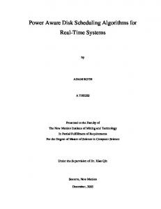
Figure 1.1: An example of two schedules for a processor whose power function is P (t) = s(t)2 . The processor executes w = 20 units of work during the interval of time [0, 4) in both schedules. The first schedule consumes E1 = 1 · 42 + 1 · 22 + 1 · 82 + 1 · 62 = 120 units of energy while the second one consumes E2 = 2 · 62 + 2 · 42 = 104 units of energy.

Power Down The power down model was formalized by Irani, Gupta and Shukla [45]. In this model, we assume that a processor can be in an active or in an inactive state. In the former state, we say that the processor is ON and that it consumes an amount of energy for being active even if nothing is executed while, in the latter state, we say that it is OFF,

4


it consumes less (or no) energy and no execution is possible. A processor can execute a job only when it is active. For simplicity, let c be the power consumption, i.e. the energy consumption per unit of time, of the processor when it is active and assume that no energy is consumed when it is inactive. The processor can save energy by turning into the inactive state during the idle periods where there are no jobs to be executed. However, an amount of energy L is dissipated for switching back from the inactive to the active state. If a processor is active for t units of time and it performs x transitions from the inactive to the active state, then its energy consumption is E =t·c+x·L Note that, the maximum amount of time that the processor can execute any job is equal to t.

0

1

2

3

4

time

5

0

ON

1

ON

2

3

OFF

4

5

time

ON

Figure 1.2: An example of two schedules for a processor which has to execute some jobs during the intervals of time [0, 1) and [4, 5). Its power consumption is c = 1 in the active state. The transition cost from the inactive to the active state is L = 2 units of energy. In the first schedule, the processor stays active during the whole interval [0, 5) and it consumes E1 = 5 · 1 + 0 · 2 = 5 units of energy. In the second schedule, it transitions to the inactive state at the time t = 1 and goes back to the active state at the time t = 4 and it consumes E2 = 2 · 1 + 1 · 2 = 4 units of energy.

Power Down with Speed Scaling There exists a hybrid model which combines speed scaling with power down mechanisms which was also introduced by Irani, Shukla and Gupta [47]. In this model, at time t, the processor’s speed-to-power function is defined as Q(t) = s(t)α + c where the speed s(t) and the constant α come from the standard speed scaling setting while c > 0 is a constant that specifies the additional power consumed at each time for being in the active state. In the inactive state, no energy is consumed. Moreover, there is an energy consumption L incurred for switching from the inactive to the active state. Continuous Thermal Model with Speed Scaling In the context of speed scaling, there exists a model for measuring the evolution of the processor’s temperature which was introduced by Bansal, Kimbrel and Pruhs [16] and

1.1. Energy and Thermal Models

5

we refer to this model as the continuous thermal model. According to this model, the increase of the temperature is proportional to the power supplied to the processor. Moreover, the processor’s cooling is assumed to be proportional to the difference between its temperature and the ambient temperature (Newton’s law of cooling). The ambient temperature Θ0 is constant and the processor’s temperature is never below Θ0 . Furthermore, the temperature scale is such that Θ0 = 0. Then, a first-order approximation for the rate of change Θ′ (t) of the temperature Θ(t) at time t is Θ′ (t) = b · Q(t) − c · Θ(t) where Q(t) is the power consumption, i.e. the instantaneous energy consumption, at time t and b, c ≥ 0 are constants. We refer to the constant c as the cooling parameter of the device. A consequence of the Newton’s law of cooling is that if the processor is supplied no power, then its temperature is reduced by a constant fraction every 1/c units of time. Discrete Thermal Model The discrete thermal model was introduced by Chrobak, Dürr, Hurand and Robert [30]. Note that this model is not combined with speed scaling. The main assumption is that some jobs require more effort to be executed than others and, thus, more heat is generated for their execution. So, each job is associated with a heat contribution which reflects the impact of the job to the temperature when the job is executed. Moreover, the processor’s cooling occurs according to the Newton’s law of cooling. That is, the processor’s temperature is reduced at a rate proportional to the difference of its current temperature and the ambient temperature of the processor’s surroundings which is, without loss of generality, equal to zero. Furthermore, the thermal behavior of a processor depends on the technical characteristics of the processor. In order to model this, we associate each processor with constant which we call its cooling factor. For simplicity, we assume that the time is partitioned into unit length time slots and at every such time slot either a single job is executed during the whole slot or the processor is idle. Formally, let us consider a processor with cooling factor c. Assume that, during the time slot [t, t + 1), the processor executes a job with heat contribution h. Let Θ(t) and Θ(t + 1) be the temperatures at times t and t + 1, respectively. Then, we have that Θ(t + 1) =

Θ(t) + h c

If the processor is idle, then the processor’s temperature is modified as if a job of zero heat contribution is executed. That is, if the processor is idle during [t, t + 1), then Θ(t + 1) =

Θ(t) c

At this point notice that Chrobak et al. [30] studied a normalization of the discrete thermal model in which the processors have c = 2 and the jobs have heat contributions in the interval [0, 2]. In fact, this is the case we consider in this thesis.

6


0

0.75

0.375

1.5 0

0.888

0.444

1.4 1

2

temperature

0.872

0

1.3 3

4

0.7 1.4

5

0

time

1

0.5

1.3 1

1 1.5

2

3

4

Figure 1.3: An example of two schedules for a processor whose cooling factor is c = 2. In both schedules, the processor executes three jobs with unit processing times and heat contributions 1.5, 1.4 and 1.3, respectively. Note that the temperature does not exceed the value 1 in any schedule.

1.2

Problem Definitions

In this section, we formally establish the setting for the scheduling problems considered in this thesis. Note that a scheduling problem is specified by a set of jobs, a processing environment and an optimization goal. Typically, a scheduling problem consists of a set of n jobs J = {J1 , J2 , . . ., Jn }. Every job Jj has an amount of work (or processing requirement) wj which must be executed for it. Moreover, each Jj is associated with a release date (or arrival time) rj and a deadline dj meaning that it can only be executed during the interval [rj , dj ). We say that Jj is active during [rj , dj ) and that [rj , dj ) is the active interval of Jj . In general, we tackle problems such that the parameters of the jobs are arbitrary. However, we sometimes restrict our attention to special cases in which some parameters might be related. First of all, we consider problems where one of the jobs’ parameters is equal for all the jobs. For example, we study a problem such that all the jobs have equal works, i.e. wj = wj ′ for each pair of jobs Jj , Jj ′ , which might arise in systems that execute the same type of jobs. Furthermore, we consider problems where the active intervals of the jobs have special structures. In agreeable instances, for every couple of jobs Jj and Jj ′ such that rj < rj ′ , it must be the case that dj ≤ dj ′ . This kind of instances include the ones where all the jobs have active intervals of equal size and there is a sort of fairness among the jobs. We also address problems where the active intervals of the jobs have a laminar structure, that is, for every couple of jobs Jj and Jj ′ such that rj < rj ′ , it holds that either dj ≥ dj ′ or dj ≤ rj ′ . Note that laminar instances occur if the jobs are created by recursive calls of a program.

r1

d1 r2

d2 r3

d3 r4

d4

Figure 1.4: An example of an agreeable instance.

1.2. Problem Definitions

r5 r3 r1

7

d5 r7

d7

r8 d3 r4

d8 d4 d1 r2

d2

Figure 1.5: An example of a laminar instance.

In a given scheduling problem, we may or not allow preemptions and migrations of the jobs. When preemptions of jobs are permitted, a job may start its execution, be suspended and resumed later from the point of suspension. In computer systems with several processors where the jobs can be preempted, if migrations of jobs are allowed, then one job may be executed by more that one processors. However, each job can only be executed by at most one processor at each time. For certain types of applications, there are precedence constraints among the jobs. If the job Jj is constrained to precede the job Jj ′ , then Jj ′ cannot start its execution until Jj is completed. The precedence relations among the jobs are represented by a directed acyclic graph G = (V, A). The set of vertices V of this graph contains one vertex for each job and there is an arc (Jj , Jj ′ ) if and only if there is a constraint according to which Jj must precede Jj ′ . In general, we consider different processing environments on which the jobs must be executed. In all the cases, a processor can only execute at most one job at each time. First, we consider environments with a single processor. Small portable devices are included in this type of environments. Today, for improving the performance of modern computing systems, designers use parallelism, i.e. multiple processors running at lower frequencies but offering better performances than a single processor. So, we also study multiprocessor environments consisting of a set of m processors P = {P1 , P2 , . . . , Pm } which run in parallel and they obey to the same speed-to-power function Q(t) = s(t)α . Another characteristic of the multiprocessor computing systems is that they tend to be heterogeneous consisting of processors of different types. Heterogeneity offers the possibility of further improving the performance of the system by allowing the execution of a job on the most appropriate type of processor. So, we also consider heterogeneous environments with special-purpose processors designed for particular types of jobs. In such environments, each processor Pi satisfies its own speed-to-power function Qi (t) = s(t)αi . Furthermore, a processor Pi may execute a job Jj more efficiently than another processor Pi′ . That is, Pi might need to execute less work than Pi′ in order to complete Jj . Therefore, each job Jj is associated with a set of values wi,j which correspond to the amount of work that the processor Pi has to execute in order to complete Jj . Additionally, every job Jj might have processor-dependent release dates ri,j and deadlines di,j . Scheduling problems with processor-dependent release dates and deadlines have been studied in the literature to model the situation in which the processors are connected by a network. In this case, it is assumed that every job is initially available at some processor and a transfer time must elapse before it becomes available for a new processor. The transfer time is reflected by an increase in the release date and the deadline.

8


In this thesis, we also consider a special type of processing environments known as shop environments. A typical shop environment consists of a set of m special-purpose parallel processors P = {P1 , P2 , . . . , Pm }. There is a set of n jobs J = {J1 , J2 , . . . , Jn } and, now, every job Jj ∈ J consists of nj operations O1,j , O2,j , . . . , Onj ,j . Every operation Ok,j has an amount of work wk,j . The processors in P are special-purpose in the sense that each processor Pi is designed to execute a particular type of operations. Therefore, every operation Ok,j is associated with a processor Pi on which it must be entirely executed. In a shop environment we assume that all the operations of a job access a common resource which is dedicated to that job. As a result, two operations of the same job cannot be executed simultaneously. We consider two kinds of shop environments, namely the open shop and the job shop. In an open shop environment, each job Jj can have at most one operation on each processor. In a job shop environment, a job Jj can have more than one operations on the same processor and there are precedence constraints among the operations of each job in the form of a chain. Specifically, the operations of the job Jj are numbered as O1,j , O2,j , . . . , Onj ,j and they must be executed in this order. That is, the operation Ok+1,j can start only once the operation Ok,j has finished. Next, we elaborate on the optimization goals of the scheduling problems that we study in this thesis. Firstly, we consider the objective of minimizing the total energy consumption. Recall that our study of the energy is based on the model of Yao et al. [62] by performing speed scaling. In most of the energy-related problems studied in this thesis, there is always an optimal schedule where each job Jj is executed with a single speed sj and this comes from the convexity of the speed-to-power function. In such schedules, we only have to define one speed for each job and the energy consumption for executing a job Jj is Ej = wj sα−1 . Therefore, our objective function is to minimize j q q α−1 E = Jj ∈J Ej = Jj ∈J wj sj . In the context of shop environments, it holds that each operation Ok,j is executed at a constant speed sk,j and the total energy consumption in q α−1 , where O is the set of all the operations. an optimal schedule is Ok,j ∈O wk,j sk,j Moreover, we study objective functions related with the thermal management. Recall that, in all the temperature aware scheduling problems that we tackle in this thesis, we adopt the discrete thermal model of Chrobak et al. [30] and, in this model, each job Jj is associated with a heat contribution hj . We, first, have to ensure that the processors’ temperature does not become too high at any time. In order to accomplish this, we consider scheduling problems where the objective is to minimize the maximum temperature Θmax attained at any time, i.e. Θmax = maxt∈T {Θ(t)}, where T is the time horizon. Another objective that we address and concerns the overall thermal behavior of q a computing system is the minimization of the average temperature t∈T Θ(t). Finally, we consider scheduling problems where the goal is to achieve high performance under energy or thermal limitations. Specifically, we try to optimize some performance metric under either a budget of energy E or a temperature threshold Θ which must not be exceeded. In general, good performance means that the completion times of the jobs are as low as possible. We denote the completion time of the job Jj by Cj . There exist many well-known performance metrics of a schedule in the bibliography. A first metric is the makespan Cmax which corresponds to the time at which the last job completes, i.e. Cmax = maxJj ∈J {Cj }. Clearly, we would like to construct schedules with

1.3. Notation for Scheduling Problems

9

minimum makespan. A generalization of the makespan is the maximum lateness of a schedule. When this objective is considered, we assume that, once the job Jj has been completed, an additional amount of time qj ≥ 0 has to elapse until it is delivered. The parameter qj is known as the delivery time of the job. Then, the lateness of a job Jj is defined as Lj = Cj + qj and the maximum lateness of the schedule is the maximum lateness among the jobs, i.e. Lmax = maxJj ∈J {Lj }. The objective now is to minimize the maximum lateness. Another classical metric of the quality of a schedule is the average (or total) completion q time Jj ∈J Cj of all the jobs. In the literature, there exists a generalization of this q objective, namely the total flow time Jj ∈J Fj of the jobs, where the flow time of a job is defined as Fj = Cj − rj . We also consider the weighted versions of these objectives. In this case, each job Jj has a weight βj > 0 which specifies its relevant importance with respect to the other jobs. The higher the weight, the higher the importance of the job is. q q A schedule with good performance should minimize either Jj ∈J βj Cj or Jj ∈J βj Fj . In energy-efficient scheduling problems, another type of objective functions is to optimize a linear combination of the energy and a performance metric. For instance, we consider problems in which we would like to minimize the energy consumption plus β times the maximum lateness, where β > 0 is a parameter specifying the relevant importance between the energy and the maximum lateness. The motivation of such a problem comes from an economic viewpoint. Specifically, we assume that we are willing to pay β units of energy in order to get a reduction of one unit of maximum lateness. So, in order to minimize our cost, it suffices to minimize the maximum lateness plus β times the energy.

1.3

Notation for Scheduling Problems

In this section, we describe a notation for energy and temperature aware scheduling problems which is a natural adaptation of the well-known three-field notation of Graham, Lawler, Lenstra and Rinnooy Kan [37] for classical scheduling problems. According to this notation, a scheduling problem is denoted by an expression with three fields in the form f1 |f2 |f3 . The field f1 corresponds to the processing environment, the field f2 concerns the jobs’ characteristics and the field f3 specifies the objective function. In the field for the processing environment f1 , we add the parameter S to specify that the processors are speed-scalable or the parameter T for the problems under the discrete thermal model. If these terms are omitted, then we consider a classical scheduling problem without energy and thermal considerations where each job Jj has a fixed processing time. In order to indicate the processing environment, we use one of the following parameters.

10

Chapter 1. Introduction 1 P R O J

Single Processor Homogeneous Parallel Processors Heterogeneous Parallel Processors Open Shop Job Shop

Table 1.1: Processing Environments for the 1st field of the 3-field Notation

As far as the job characteristics are concerned, we use wj (or wi,j in the case of heterogeneous or shop environments) for specifications on the works of the jobs (or operations). We use these parameters if we want to indicate that the jobs have equal works by writing wj = w. If we omit the term, then the jobs (or the operations) have arbitrary works. In problems without speed scaling, i.e. the ones under the discrete thermal model or the ones without energy/thermal considerations, we use pj for the processing times of the jobs instead of wj . We write rj and dj (or ri,j and di,j ) for clarifications concerning the release dates and the deadlines of the jobs. If the parameter rj is not included in the 3-field notation, then all the jobs are available to the system at the time t = 0. Otherwise, if the jobs do not have equal release dates, then we have to add rj . By omitting dj , we mean that the jobs do not have deadlines. In order to indicate that the jobs have equal or arbitrary deadlines, we write dj = d and dj , respectively. In problems under the discrete thermal model, we add the term hj to specify that every job has a heat contribution. Note that, in the case of the maximum lateness objective, each job Jj is associated with a delivery time qj and we do not add anything in the field f2 . By including the term agrbl or lmnr, the problem is restricted to agreeable or laminar instances, respectively. The default setting in our notation is that we do not allow preemptions and migrations of the jobs. In order to permit them, we must include the parameters pmtn or mgtn, respectively, in f2 . Finally, we add the term prec so as to indicate that there are precedence constraints among the jobs. The possible expressions that concern the jobs’ characteristics are summarized in the following table. wj = w (or wi,j = w) pj = p rj (or ri,j ) dj (or di,j ) dj = d hj agrbl lmnr pmtn mgtn prec

Equal-Work Jobs (Operations) Equal Processing Times Arbitrary Release Dates Arbitrary Deadlines Equal Deadlines Heat Contributions Agreeable Instances Laminar Instances Preemptions Preemptions and Migrations Precedence Constraints

Table 1.2: Expressions for the 2nd field of the 3-field Notation

Finally, in the field f3 , we specify the objective function of the problem. In the case where the objective function is a performance-related objective function with a constraint

1.4. Algorithm Analysis

11

on the energy or the temperature, we have to indicate whether we have a budget of energy or a temperature threshold by adding in parantheses the symbols E or Θ, respectively. The possible objective functions are stated in the following table. E Θmax q Θt Cmax (E) or Cmax (Θ) Cmax + βE Lmax (E) or Lmax (Θ) Lmax + βE q q Cj (E) or Cj (Θ) q Cj + βE q q wj Cj (E) or wj Cj (Θ) q wj Cj + βE q q Fj (E) or Fj (Θ) q Fj + βE q q wj Fj (E) or wj Fj (Θ) q wj Fj + βE

Energy Maximum Temperature Average Temperature Makespan Makespan plus Energy Maximum Lateness Maximum Lateness plus Energy Average Completion Time Average Completion Time plus Energy Weighted Average Completion Time Weighted Average Completion Time plus Energy Total Flow Time Total Flow Time plus Energy Weighted Total Flow Time Weighted Total Flow Time plus Energy

Table 1.3: Objective Functions for the 3rd field of the 3-field Notation

For example, S, 1|rj |Lmax (E) is the problem of minimizing the maximum lateness of a set of jobs with release dates where the objective is the minimization of the maximum lateness and there is a budget of energy. In the problem S, R|ri,j , di,j , mgtn|E, we would like to minimize the energy of a set of jobs with processor-dependent release dates and deadlines on fully heterogeneous parallel processors where preemptions and migrations of jobs are allowed. Finally, in T, P|pj = 1, dj = d, hj |Θmax , our objective is to minimize the maximum temperature on parallel identical processors under the discrete thermal model, where there is a set of unit-length jobs with equal release dates and deadlines.

1.4

Algorithm Analysis

Tractability and Approximation Algorithms The running time of an algorithm is the number of elementary operations it performs such as primitive arithmetic operations, primitive logic operations etc. A polynomial algorithm for a given optimization problem, is an algorithm which produces an optimal solution for the problem in time polynomial the size of its instance |I|, i.e. the number of the bits needed in order to encode the instance I in a binary representation. We say that an optimization problem is tractable if it admits a polynomial algorithm. In general, there exist problems which are tractable and others which are intractable. However, there is also a class of problems, the N P-complete problems, for which we do not know whether they are tractable or not. A basic aspect of the N P-complete problems is that they all have, in a sense, equivalent difficulty. Specifically, if there was a tractable

12


N P-complete problem, then this would imply tractability for every other N P-complete problem. On the other hand, if there was an intractable N P-complete problem, then this would imply intractability for every other N P-complete problem. The question of the tractability of N P-complete problems in a major open question in computer science and it is known as the P = N P question. In general, it is conjectured that P = Ó NP which means that the N P-complete problems are intractable. The opposite is considered unlikely. The equivalence property of the N P-complete problems, provide a way of showing that a problem is N P-complete through a so called N P-completeness reduction. Specifically, assume that we are given an optimization problem Π and that we know that another problem Π′ is N P-complete. In order to show that Π is N P-complete, it suffices to show that if we are given an optimal polynomial algorithm for Π′ , then we can use it as a black box an define an optimal algorithm for Π. Unless P = N P, we do not expect a polynomial-time algorithm for an N P-complete problem. However, many N P-complete problems are very important in practice and we would like to cope with them. One way to solve such a problem is by an approximation algorithm. An approximation algorithm is a polynomial-time algorithm which does not produce an optimal solution but a near-optimal solution instead. Formally, consider an optimization problem for which we are given a polynomial-time algorithm A. For a given instance I of the problem, we denote by CA (I) and COP T (I) the cost of the algorithm’s solution and the cost of the optimal solution, respectively. Then, A is a ρ-approximation algorithm if, for any possible instance I of the problem, it holds that CA (I) ≤ ρ · COP T (I) If a problem admits a ρ-approximation algorithm, then we can compute, in polynomial time, a solution whose cost is at most ρ times the cost of an optimal solution. We refer to the value ρ as the approximation ratio of the algorithm A. For some N P-complete problems, we may define a polynomial time approximation scheme (PTAS) which is an algorithm that computes a solution whose cost is very close to the optimal. Formally, a PTAS is an algorithm which computes an (1+ǫ)-approximate solution in time polynomial to the size of the instance, for any ǫ > 0. When an algorithm computes an (1 + ǫ)approximate solution in time polynomial to the size of the instance and 1/ǫ, for any ǫ > 0, then we call it a fully polynomial time approximation scheme (FPTAS). Online Algorithms Our discussion so far has lied around the offline setting. That is, we assume that the algorithm knows the entire instance before solving a problem. This is not the case in the online setting in which the algorithm does not know all the instance in advance but the knowledge comes over the time while the algorithm runs. In order to evaluate the performance of online algorithms for some optimization problem, we adopt the competitive analysis according to which the solution of an algorithm is compared with the solution of an optimal offline algorithm. Assume that we are given an online algorithm A for some optimization problem. For a given instance I of the problem, let CA (I) and COP T (I) the cost of an algorithm’s solution and the cost of the optimal offline solution, respectively.

1.5. Related Work

13

We say that A is ρ-competitive if, for any possible instance I of the problem, it holds that CA (I) ≤ ρ · COP T (I)

1.5

Related Work

In this section, we will describe existing work on energy and temperature aware scheduling problems which is closely related to this thesis. Initially, we present part of the literature for speed scaling problems on a single processor, on homogeneous parallel processors and on heterogeneous parallel processors. We also briefly describe existing work on the power down model and the hybrid model that combines speed scaling with power down. Note that there exist some surveys in the context of energy-efficient scheduling by Albers [2] and by Irani and Pruhs [46]. Finally, we present existing work for thermal management problems. Speed Scaling on a Single Processor Offline Energy Minimization. The theoretical study of speed scaling was initiated in a seminal paper by Yao et al. [62] who considered the single processor problem of scheduling a set of jobs with release dates and deadlines, preemptively, so as to minimize the total energy consumption, i.e. S, 1|rj , dj , pmtn|E. The authors showed that the particular problem is polynomially solvable by constructing an optimal algorithm whose running time is O(n3 ). Later, Li et al. [52] proposed a faster algorithm with time complexity O(n2 log n). When the instances are restricted to be laminar, Li et al. [51] showed that the problem can be solved in O(n) time. Antoniadis et al. [9] were the first to consider the non-preemptive energy minimization problem S, 1|rj , dj |E for which they observed that it is strongly N P-hard even for laminar instances. They also presented a 24α−3 -approximation algorithm for laminar instances and a 25α−4 -approximation algorithm for general instances. Furthermore, the authors noticed that the problem can be solved optimally in polynomial time when the instances are agreeable by observing that the optimal preemptive schedule produced by the algorithm in [62] is always non-preemptive.

14

Chapter 1. Introduction Problem S, 1|rj , dj , pmtn, lmnr|E S, 1|rj , dj , pmtn|E S, 1|rj , dj , agrbl|E S, 1|rj , dj , lmnr|E S, 1|rj , dj |E

Complexity Polynomial Polynomial Polynomial N P-hard N P-hard

Best-known Algorithm O(n) [51] O(n2 log n) [52] O(n3 ) [9] [62] 4α−3 2 -approximation [9] 25α−4 -approximation [9]

Table 1.4: Offline Energy Minimization

Online Energy Minimization. Yao et al. [62] considered also the online version of the problem S, 1|rj , dj , pmtn|E in which each job is known at its release date. They proposed two reasonable online algorithms, namely the AVR (Average Rate) and the OA (Optimal Available). For AVR, they established a competitive ratio of 2α−1 αα and they showed that it cannot be better than αα . Later, Bansal et al. [12] presented a more elementary (simpler) proof of the fact that AVR is 2α−1 αα -competitive and they concluded that this ratio is almost tight by showing that AVR’s competitive ratio cannot be less than (2 − δ)α−1 αα , where δ approaches zero as α goes to infinity. In another work, Bansal et al. [16] proved that OA is αα -competitive and they showed that this ratio is essentially tight for OA, because there is an instance such that the energy consumption of the OA’s schedule is αα times the energy consumption of an optimal offline schedule. α α α ) e , In the same work, they proposed the BKP algorithm with competitive ratio 2( α−1 which is better than OA for α ≥ 5. Finally, Bansal et al. [14] defined the qOA algorithm α which is 2e1/24 α1/4 -competitive. Moreover, the authors showed that qOA cannot be better α−1 α−1 than 4 α (1 − α2 )α/2 -competitive and they established a generic lower bound e α on the competitive ratio of any deterministic algorithm for the problem. Algorithm AVR OA BKP qOA Any Deterministic

Competitive Ratio Lower Bound Upper Bound (2 − δ)α−1 αα [12] 2α−1 αα [62] αα [16] αα [16] α α α 2( α−1 ) e [16] 2 α/2 4α −1 4α [14] [14] α (1 − α ) 2e1/2 α1/4 eα−1 α [14]

Table 1.5: Online Energy Minimization

Next, we consider single processor speed scaling problems where the objective is a performance criterion under a budget of energy. Offline Average Completion Time Minimization. The first work in this context was by Pruhs et al. [56] who considered the problem of minimizing the average completion time under a budget of energy and proposed an O(n2 log Eǫ ) polynomial time algorithm for the special case where the jobs have equal works, where E is the energy budget and ǫ

1.5. Related Work

15

is the desired accuracy. In another work, Albers et al. [5] proposed a simplified algorithm for the problem of minimizing the average completion time plus energy which is based on dynamic programming. These results hold for the objective of minimizing the total flow time under a budget of energy as well. Megow et al. [54] considered the weighted version of the average completion time objective. For the case where all the jobs have equal release dates, they established a polynomial time approximation scheme (PTAS) and, interestingly, they showed that this q α−1 problem is equivalent to the problem 1|| wj (Cj ) α in which no speed scaling is performed and every job has a fixed processing time. The complexity status of the latter q problem is an open question. Independently from [54], the equivalence of 1|| wj Cj (E) q α−1 with 1|| wj (Cj ) α was also shown by Vásquez [60]. For the preemptive problem q S, 1|rj , pmtn| wj Cj (E), where the jobs have arbitrary release dates, Megow et al. [54] proposed a (2 + ǫ)-approximation algorithm. Problem q S, 1|rj , pj = p| Cj (E) q S, 1|| wj Cj (E) q S, 1|rj , pmtn| wj Cj (E)

Complexity Polynomial ? N P-hard

Best-known Algorithm O(n2 log Eǫ ) [56] PTAS [54] (2 + ǫ)-approximation [54]

Table 1.6: Offline Average Completion Time Minimization

Online Total Flow Time. For the online version of the average completion time q minimization problem with a budget of energy S, 1|rj , pmtn| Cj (E), where each job is known only once it has arrived (i.e. at its release date), it is not possible to have a constant factor competitive algorithm even if we consider instances with unit-work jobs. A formal proof of this invariant was presented by Bansal et al. [17] where they proposed an adversarial strategy which makes any deterministic algorithm run out of energy. For this reason, in order to optimize both the average completion time and the energy in the online setting, Albers et al. [5] proposed to study problems where the objective function is the sum of the two objectives. Albers et al. [5] initiated the study of the online non-preemptive energy-efficient q problem S, 1|rj | Fj + E for which they showed that the best possible algorithm cannot be better than Ω(n1−1/α )-competitive. So, they considered the case where the jobs have unit works and they proposed an O(1)-competitive algorithm whose competitive ratio α α ) . Next, Bansal et al. [17] improved this result by showing that the is 8(1 + Φ)α ( α−1 algorithm in [5] is 4-competitive for unit-work jobs. Since an optimal preemptive schedule is non-preemptive for unit-work jobs, the competitive ratio of the algorithm in [5] is the same for the preemptive case as well. q Bansal et al. [17] studied the more general problem S, 1|rj , pmtn| Fj + E where the jobs have arbitrary release dates and preemptions are allowed. They constructed an 2(α−1) }. When the value algorithm with a competitive ratio equal to (1 + ǫ) max{2, 1− 1 of α is large, this ratio is approximately 2 algorithm of competitive ratio

2( lnαα )2 .

α 1−(α−1)/(α α−1 )

α−(α−1)

α−1

Later, Lam et al. [49] proposed a better . This ratio tends to 2 lnαα for large values

16


of α. Next, Bansal et al. [15] made significant progress on this problem by presenting a 3-competitive algorithm. Finally, Andrew et al. [7] established the best online algorithm for the problem which is a slight modification of the one in [15] and which is 2-competitive. Moreover, they showed a lower bound of 2 on the competitive ratio of any algorithm in a class of reasonable algorithms. q As far as the online problem S, 1|rj , pmtn| wj Fj + E of minimizing the weighted flow time is concerned, no deterministic algorithm can be O(1)-competitive and this holds even for the classical scheduling setting where no speed scaling is performed. The proof of this negative result was due to Bansal et al. [13]. Problem q S, 1|rj | Fj + E q S, 1|rj , pmtn| Fj + E q S, 1|rj , pmtn| wj Fj + E

Lower Bound 1 Ω(n1− α ) [5]

Best-known Algorithm 2-competitive [7]

no O(1)-competitive [13]

Table 1.7: Online Total Flow Time Minimization

Offline Makespan Minimization. Bunde [28] studied the non-preemptive offline problem S, 1|rj |Cmax (E) of minimizing the makespan of a set of jobs with release dates under an energy budget. Specifically, he proposed an optimal polynomial-time algorithm with running time O(n2 ). Note that, for the preemptive case of the problem, there is always an optimal schedule which is non-preemptive. Therefore, the algorithm in [28] is optimal for the preemptive case, too. Speed Scaling on Homogeneous Parallel Processors Offline Energy Minimization. Chen et al. [29] were the first to study a multiprocessor energy-efficient scheduling problem involving speed scaling. More specifically, they proposed a polynomial-time algorithm for solving optimally the multiprocessor migratory preemptive energy minimization problem of a set of jobs with equal release dates and deadlines. The running time of their algorithm is O(n log n). Later, Bingham et al. [23] constructed an optimal algorithm for the general version of the problem S, P|rj , dj , mgtn|E where the jobs have arbitrary release dates and deadlines. The algorithm in [23] makes repetitive calls of a black-box algorithm for solving linear programs. Then, Albers et al. [4] presented a faster combinatorial algorithm which is based on a formulation of the problem as a maximum flow problem. It has to be noticed here that, independently, we presented another optimal polynomial time algorithm for the same problem which is based on the relation of the problem with the maximum flow problem. Albers et al. [6], considered the non-migratory preemptive problem of minimizing the energy of a set of unit-work jobs with arbitrary release dates and deadlines. The authors showed that this problem can be solved optimally in polynomial time if the instances are restricted to be agreeable. Moreover, they established an N P-hardness proof for the unit-work case when the release dates and the deadlines of the jobs are arbitrary and they proposed an αα 24α -approximation algorithm for it. They also produced an

1.5. Related Work

17

algorithm of the same approximation ratio for arbitrary-work instances when the jobs have either equal release dates or equal deadlines. Next, Greiner et al. [39] presented a B⌈α⌉ -approximation algorithm for the general problem S, P|rj , dj , pmtn|E with jobs having arbitrary processing requirements, where B⌈α⌉ is the ⌈α⌉-th Bell number. Very little attention has been given to the non-migratory non-preemptive problem S, P|rj , dj |E. Albers et al. [6] observed that the problem is N P-hard even in the special case where the jobs have the same release date and the same deadline. Moreover, they claimed that, for this special case of the problem, there exists a polynomial time approximation scheme (PTAS) which can be derived easily from an existing PTAS of the well-known problem P||Cmax . Problem S, P|dj = d, mgtn|E S, P|rj , dj , mgtn|E S, P|wj = 1, rj , dj , agrbl, pmtn|E S, P|wj = 1, rj , dj , pmtn|E S, P|rj , dj , pmtn|E S, P|dj = d|E

Complexity Polynomial Polynomial Polynomial N P-hard N P-hard N P-hard

Best-known Algorithm O(n log n) [29] max-flow based [4] O(mn2 log n) [6] α 4α min{α 2 , B⌈α⌉ }-approximation [6] [39] B⌈α⌉ -approximation [39] PTAS [6]

Table 1.8: Offline Energy Minimization

Online Energy Minimization. For the online version of S, P|rj , dj , mgtn|E, Albers et al. [4] proposed the online algorithms AVR and OA which are the straightforward generalizations of the corresponding algorithms for the single processor case presented α in [62]. In [4], they showed that AVR is (3α) + 2α -competitive and that OA is αα 2 competitive. Albers et al. [6] considered the online variant of the problem S, P|rj , dj , pmtn|E and restricted their attention to unit work instances. For agreeable instances, they constructed α α α a 2( α−1 ) e -competitive algorithm while, for the case where the release dates and the deadlines of the jobs are arbitrary, they developed an αα 24α -competitive algorithm. For general instances with arbitrary release dates and works, Bell et al. [21] proposed an online algorithm with competitive ratio 24α (logα P + αα 2α−1 ), where P is the ratio of the maximum work among the jobs over the minimum work. Problem S, P|pj = 1, rj , dj , mgtn|E S, P|pj = 1, rj , dj , agrbl, pmtn|E S, P|pj = 1, rj , dj , pmtn|E S, P|rj , dj , pmtn|E

Best-known Algorithm αα -competitive [4] α α α ) e -competitive [6] 2( α−1 αα 24α -competitive [6] 24α (logα P + αα 2α−1 )-competitive [21]

Table 1.9: Online Energy Minimization

18


Online Total Flow Time Minimization. For the problem S, P|rj , pmtn| Fj + E, Lam et al. [48], proposed an online algorithm whose competitive ratio is O(2α(log P + 2α )). Moreover, on the negative side, Leonardi et al. [50] showed that no deterministic algorithm can be O(1)-competitive even for processors with fixed speeds which is extended to the speed scaling setting. q

Offline Makespan Minimization. Pruhs et al. [57] studied the non-migratory multiprocessor problem S, P||Cmax (E) of minimizing the makespan of a set of jobs with equal release dates under a budget of energy and derived a PTAS for it by using as a black box an existing PTAS for the classical scheduling problem of minimizing the ℓα norm of a load balancing problem. Moreover, they considered the more general version where there are 2 precedence constraints among the jobs and they proposed an O(log1+ α m)-approximation algorithm for it. Speed Scaling on Heterogeneous Parallel Processors There does not exist much work on environments with heterogeneous processors. In [41] and [42], Gupta et al. considered the online problem of minimizing the flow time plus energy and they presented online algorithms with a constant competitive ratio which are based on resource augmentation. These works indicate that energy efficient scheduling on heterogeneous processors may be more difficult than the homogeneous case and new algorithms are required. Power Down The power down model was formalized by Irani, Gupta and Shukla [45]. Baptiste [18] considered the single processor problem of minimizing the energy of a set of jobs with release dates and deadlines. He proposed an optimal algorithm for jobs with unit processing times a FPTAS for the more general case where the jobs have arbitrary processing times and preemptions are allowed. Later, Baptiste et al. [20] proposed a faster polynomial algorithm for unit jobs and presented a polynomial algorithm for the preemptive problem with arbitrary processing times. Further results with respect to this model can be found in [8], [31] and [32]. Power Down with Speed Scaling The model that combines speed scaling with power down was first studied by Irani et al. [47] who derived a constant factor approximation for the problem of minimizing the energy of a set of jobs with release dates and deadlines. Then, Albers et al. [3] showed that the problem is N P-hard if the power function is of a particular form. They also proposed an improved approximation algorithm. Finally, Bampis et al. [11] proved that the problem is polynomially solvable for agreeable instances.

1.6. Contributions

19

Continuous Thermal Model The continuous thermal model was introduced by Bansal et al. [16]. First, they considered the offline problem S, 1|rj , dj , pmtn|Θmax of minimizing the maximum temperature and they showed that it can be solved in polynomial time by applying the Ellipsoid Alα α gorithm. In the same work, they proposed an eα 2α+1 (6( α−1 ) + 1)-competitive algorithm for the online version of the problem of minimizing the maximum temperature in which each job is known at its release date. Atkins et al. [10] developed a faster O(n2 ) combinatorial algorithm for the offline case where the jobs have equal release dates. Moreover, they defined another algorithm for the online case with arbitrary release dates whose e (2 + 3eαα ). This algorithm is better than the one in [16] for some competitive ratio is e−1 values of α, e.g. when the cube-root rule α = 3 holds. Discrete Thermal Model The study of temperature-aware scheduling problems with respect to the discrete thermal model was initiated by Chrobak et al. [30] who considered the single-processor problem of finding schedules with maximum throughput for unit jobs. They showed that the problem is strongly N P-hard even when the jobs have equal release dates and deadlines and unit processing times and the processor’s cooling factor is c = 2. In this problem it is possible that we cannot schedule feasibly all the jobs between their release dates and their deadlines and our objective is to maximize the number of jobs which are completed on time. The N P-hardness proof in [30] implies that the problems T, 1|pj = 1, dj = d, hj |Θmax q (maximum temperature minimization), T, 1|pj = 1, hj | Fj (Θ) (total flow time minimization) and T, 1|pj = 1, hj |Cmax (Θ) (makespan minimization) are also N P-hard. For the problem of minimizing the total flow time, Birks et al. [27] proposed a 2.618-approximation algorithm for the special case where all the jobs are released at the same time and they established an Ω(n1/2−ǫ )-inapproximability result for instances with arbitrary release dates, where ǫ > 0. Chrobak et al. [30] also considered the online problem of maximizing the throughput in which the jobs arrive over time and they proposed an algorithm with constant competitive ratio. Then, Birks et al. [24], [25], [26] addressed several generalizations of the online throughput maximization problem. In fact, in [24] the weighted throughput objective is considered. In [25] the cooling effect is generalized by multiplying the temperature by 1/c, where c > 1, instead of one half, while in [26] the jobs have equal (non-unit) processing times. Finally, Dürr et al. [34] considered the offline problem of maximizing the throughput and proposed positive and negative results on the approximation ratio of the coolest first algorithm.

1.6

Contributions

In this section, we briefly describe the contributions of this thesis.

20


Single Processor Initially, we consider the single-processor non-preemptive energy minimization problem S, 1|rj , dj |E. Recall that the study of this problem was initiated recently and it was observed that the problem is strongly N P-hard [9]. Antoniadis et al. [9] proposed a constant factor approximation algorithm for the non-preemptive problem through a transformation to the unrelated machine scheduling problem with the ℓα -norm objective. Here, we explore the idea of transforming an optimal preemptive schedule to a non-preemptive one and we show that, for unit-work instances, this approach leads to an improved approximation ratio. In Section 2.1, we derive some properties of optimal preemptive schedules produced by the algorithm of Yao et al. [62]. Next, in Section 2.2 we prove that the preemptive optimal solution does not preserve enough of the structure of the non-preemptive optimal solution and, more precisely, that the ratio between the energy consumption of an optimal non-preemptive schedule and the energy consumption of an optimal preemptive one can be Ω(nα−1 ). So, with this )α -approximation algorithm, where wwmax is the ratio approach, we obtain an (1 + wwmax min min between the maximum and the minimum work among the jobs. For equal-work instances, this algorithm is 2α -approximate which is better than the 25α−4 -approximation algorithm by Antoniadis et al. [9] proposed for arbitrary work instances. Next, we follow another approach for solving S, 1|rj , dj |E which based on a reduction of the problem to the multiprocessor non-migratory preemptive energy minimization problem S, P|ri,j , di,j , pmtn|E in which the release dates and the deadlines of the jobs are processor-dependent. Our reduction allows us to prove that based on a ρ-approximation algorithm for the latter problem, we obtain a 2α−1 ρ-approximate solution for the former one. In Section 2.3, we initiate the study of the single-processor scheduling problem of minimizing the maximum lateness and the energy of a set of jobs. Initially, we address the problem of minimizing the maximum lateness under a budget of energy and we propose an optimal polynomial-time algorithm for the special case in which the jobs have equal release dates, i.e. for the problem S, 1||Lmax (E). This algorithm constructs greedily an optimal solution satisfying the KKT conditions applied to a convex programming formulation of the problem. Subsequently, we show that the problem S, 1|rj |Lmax (E) in which the jobs may have arbitrary release dates is strongly N P-hard. Finally, we move our attention to the online setting in which each job is known at its release date. Clearly, given the existing literature (see Bansal et al. [17]), we do not expect a constant factor competitive algorithm for the problem of minimizing the maximum lateness under a budget of energy. For this reason, following the approach of Albers et al. [5] for the average completion time objective, we study the online problem S, 1|rj |Lmax + βE of minimizing a linear combination of the maximum lateness and the energy and we obtain a 2-competitive algorithm by applying a batched scheduling strategy [59]. Homogeneous Parallel Processors Subsequently, we study multiprocessor scheduling problems on homogeneous parallel processors. Initially, we address the multiprocessor problem of minimizing the energy of a set of jobs on parallel homogeneous processors where preemptions and migrations of jobs

1.6. Contributions

21

are allowed, i.e. S, P|rj , dj , mgtn|E. Recall that the previously best known algorithm for this problem uses an optimal algorithm for solving linear programs as a black box. So, in Section 3.1, we present a faster combinatorial algorithm which is based on maximum flow computations. Note that, independently from the algorithm presented in this thesis, another algorithm was proposed for the same problem by Albers et al. [4] which also explores the relation of the problem with the maximum flow problem. These results introduce the use of maximum flow formulations in the context of speed scaling. In order to establish the optimality of our maximum flow based algorithm and of the one of Albers et al. [4] for S, P|rj , dj , mgtn|E, we need a series of technical lemmas. We present an alternative algorithm for S, P|rj , dj , mgtn|E which is based on a formulation of the problem as a minimum convex cost flow problem. This algorithm constructs an optimal schedule through a single convex cost flow computation and its analysis is much simpler. Finally, in Section 3.2, we initiate the study of the multiprocessor energy minimization problem in which migrations and preemptions of the jobs are not allowed. As for the single processor case, we study the idea of transforming optimal migratory preemptive schedules to non-preemptive ones. While for general instances we do not hope to obtain a constant-factor approximation algorithm by using this idea, we obtain a constant-factor approximation algorithm for agreeable instances. We propose an algorithm which starts by computing an optimal multiprocessor migratory preemptive schedule for the problem S, P|rj , dj , mgtn|E. In this way, it calculates a processing time for each job. By speeding up the execution of each job, it constructs a feasible non-preemptive schedule and we obtain a (2 − m1 )α -approximation algorithm for agreeable instances, i.e. S, P|rj , dj , agrbl|E. Heterogeneous Parallel Processors Next, we study scheduling problems on heterogeneous processors in which each processor satisfies its own speed-to-power function and the jobs have processor-dependent processing requirements. As Gupta et al. [41] noticed, scheduling problems with heterogeneous processors seem to require new techniques in order to be solved than their corresponding with homogeneous processors. In order to solve energy minimization problems in such environments, we introduce the idea of solving and rounding configuration linear programs. First we consider the energy minimization problem S, R|wi,j , ri,j , di,j , mgtn|E, where preemptions and migrations of the jobs are allowed. In order to obtain an algorithm for this problem, we formulate the problem as a configuration linear program (LP) with an exponential number of variables. This configuration LP cannot be solved directly in polynomial time. However, we show how to apply the Ellipsoid algorithm to its dual LP and, then, solve the configuration linear program with only a polynomial number variables. In this way, we obtain an (OP T + ǫ)-approximate solution in time polynomial to the size of the problem’s instance and 1/ǫ. Next, we move our attention to the problem S, R|wi,j , ri,j , di,j , pmtn|E in which preemptions of jobs are allowed but migrations are not permitted. This problem can be formulated as an integer configuration LP. In order to solve this LP, we show how to solve its fractional relaxation in polynomial time by applying the Ellipsoid algorithm.

22


Then we trasform the optimal fractional solution to a feasible integral one by applying ˜α (1 + ǫ)-approximate, where B ˜α is the generrandomized rounding. Our algorithm is B alized Bell number. Subsequently, we show that the algorithm can be made faster by solving a more compact LP and then transforming the optimal solution obtained into an optimal fractional solution of the configuration LP. Shop Environments Another type of computing environments considered in this thesis are the so called shop environments. Initially, we study the energy minimization problem S, O|dj = d, pmtn|E in an open shop environment, where preemptions of the operations are allowed. For this problem we follow two different approaches. Firstly, we derive an optimal algorithm for S, O|dj = d, pmtn|E based on a primaldual schema in the setting of convex programming and KKT conditions. Note that there exists much work on the use of the primal-dual method in the field of combinatorial optimization. However, most of this work concerns applications of the method in linear programming. This method was applied only recently to the more general setting of convex programming by Devanur et al. [33] and Vegh [61]. Because of the KKT conditions, the dual variables are related with the primal ones through a set of equalities. So, we obtain an optimal primal solution by properly adjusting the dual variables. We prove that our algorithm converges to the optimal solution but we are unable to prove that it converges in polynomial time. Therefore, we performed a series of experiments showing that the number of iterations of our algorithm increases linearly with the number of jobs n when it holds that m Ó= n, where m is the number of the processors. However, in the very specific case where n = m, our algorithm is slower. We are also interested in the comparison of the execution time of our method with respect to the time spent by a commercial solver which solves directly the corresponding convex program. Our second approach for solving S, O|dj = d, pmtn|E is to formulate of the problem as a minimum convex cost flow problem. The main technical difficulty behind our algorithm is that it is not obvious how the amount of flow F , which is a parameter for the minimum convex cost formulation, can be computed. However, we show a way for computing F through several minimum convex cost computations. ˜αmax -approximation algorithm for the energy minimization probNext, we present a B lem S, J|wi,j , ri,j , di,j , pmtn|E in a job shop environment. This algorithm is based on solving the fractional relaxation of an integer configuration LP and applying randomized rounding in order to obtain a feasible integral solution. Temperature Aware Scheduling Finally, we consider scheduling problems in which our focus is no longer the management of the energy but the management of the temperature. In this thesis, we adopt the discrete thermal model introduced by Chrobak et al. [30] and we initiate the study of several multiprocessor scheduling problems such that either there is a temperature threshold which must not be exceeded, or the temperature is the optimization goal itself. Firstly, we address the problem T, P|pj = 1, hj |Cmax (Θ) of minimizing the makespan under a temperature threshold and we solve it by transforming any instance of the

1.6. Contributions

23

problem to an instance of the classical makespan minimization problem P||Cmax in which there are no thermal considerations. Then, by using any ρ-approximation algorithm for P||Cmax as a black box, we obtain a 2ρ-approximation algorithm for the temperature-aware problem. Given that there exists a polynomial time approximation scheme (PTAS) for P||Cmax , our transformation leads to a (2 + ǫ)-approximation ratio for T, P|pj = 1, hj |Cmax (Θ) within a running time that is polynomial in n and expo1 )nential in 1/ǫ. If instead of the PTAS we use the standard LPT rule which is ( 34 − 3m approximate for P||Cmax , we present a tighter analysis, improving the 2ρ-approximation 1 ratio to ( 37 − 3m ), while the overall running time is O(n log n). Subsequently, we study the problem T, P|pj = 1, dj = d, hj |Θmax of minimizing the maximum temperature and we propose a 34 -approximation algorithm. Moreover, we show that our algorithm cannot not have better approximation ratio and our analysis is essenq tially tight. Then, we move our attention to the problem T, P|pj = 1, dj = d, hj | Θt of minimizing the average temperature and we show that it is polynomially solvable.

24

Chapter 1. Introduction The results of this thesis come from the following publications: • E. Bampis, A. Kononov, D. Letsios, G. Lucarelli and M. Sviridenko. Energy Efficient Scheduling and Routing via Randomized Rounding. Submitted. • E. Bampis, V. Chau, D. Letsios, G. Lucarelli and I. Milis. Energy Minimization via a Primal-dual Algorithm for a Convex Program. E. Bampis, V. Chau, D. Letsios, G. Lucarelli and I. Milis. 12th International Symposium on Experimental Algorithms (SEA’13), Rome, Italy, p. 366-377, LNCS 7933, Springer, 2013. • E. Bampis, A. Kononov, D. Letsios and G. Lucarelli and I. Nemparis. From Preemptive to Non-preemptive Speed-Scaling Scheduling. 19th International Computing and Combinatorics Conference (COCOON’13), Hangzhou, China, p. 134-146, LNCS 7936, Springer, 2013. • E. Bampis, D. Letsios and G. Lucarelli. Green Scheduling, Flows and Matchings. 23rd International Symposium on Algorithms and Computation (ISAAC’12), Taipei, Taiwan, p. 106-115, LNCS 7676, Springer, 2012. • E. Angel, E. Bampis, F. Kacem and D. Letsios. Speed Scaling on Parallel Processors with Migration. 18th International European Conference on Parallel and Distributed Computing (EURO-PAR’12), Rhodes, Greece, p. 128-140, LNCS 7484, Springer, 2012. • E. Bampis, D. Letsios, I. Milis and G. Zois. Speed Scaling for Maximum Lateness. 18th International Computing and Combinatorics Conference (COCOON’12), Sydney, Australia, p. 25-36, LNCS 7434, Springer, 2012. • E. Bampis, D. Letsios, G. Lucarelli, E. Markakis and I. Milis. On Multiprocessor Temperature-Aware Scheduling Problems. Joint Conference of 6th International Frontiers of Algorithmics Workshop and 8th International Conference on Algorithmic Aspects of Information and Management (FAW-AAIM’12), Beijing, China, p. 149-160, LNCS 7285, Springer, 2012.

Chapter 2 Single Processor In this chapter, we begin the study of energy efficient scheduling problems on the basic setting of a single processor. First, in Section 2.1, we present an optimal algorithm for the preemptive energy minimization problem S, 1|rj , dj , pmtn|E which was proposed by Yao et al. [62]. Then, in )α -approximation algorithm Section 2.2, based on this algorithm, we derive an (1 + wwmax min for the non-preemptive energy minimization problem S, 1|rj , dj |E, where wmax and wmin are the maximum and the minimum work of a job, respectively. Note that our algorithm is 2α -approximate for instances in which the jobs have equal works. In Section 2.2, we also propose another approximation algorithm for the non-preemptive problem S, 1|rj , dj |E which based on a transformation of the problem to the multiprocessor energy minimization problem S, P|ri,j , di,j , pmtn|E where preemptions of jobs are allowed but migrations are forbidden. Given a ρ-approximation algorithm for the latter problem as a black box, we obtain a 2α−1 ρ-approximation algorithm for the former problem. Subsequently, in Section 2.3, we consider offline and online energy aware problems where the objective is the minimization of the maximum lateness. Initially, we consider the offline problem S, 1|rj |Lmax (E) of minimizing the maximum lateness under a budget of energy. For the special case in which the jobs have equal release dates, i.e. S, 1||Lmax (E), we propose an optimal polynomial time algorithm. Then, we show that the problem becomes strongly N P-hard when the release dates of the jobs may be arbitrary. Finally, we move our attention to the online problem S, 1|rj |Lmax + βE of minimizing a linear combination of the maximum lateness and the energy. In the online setting, each job is known when it is released. For this problem, we propose a 2-competitive algorithm which schedules the jobs in batches by applying repeatedly an optimal offline algorithm for S, 1||Lmax + E. Such an algorithm for S, 1||Lmax + E can be obtained by using the optimal offline algorithm for S, 1||Lmax (E) as a black box and applying binary search.

2.1

Energy Minimization with Preemptions

In this section, we describe an optimal algorithm for the preemptive energy minimization problem S, 1|rj , dj , pmtn|E. This algorithm was proposed by Yao et al. [62]. Moreover, we establish some properties of the schedules produced by this algorithm that we use in Section 2.2 in order to derive an approximation algorithm for the non-preemptive problem 25

26

Chapter 2. Single Processor

S, 1|rj , dj |E. An instance of the problem S, 1|rj , dj , pmtn|E consists of a set of jobs J = {J1 , J2 , . . . , Jn } which have to be scheduled by a single processor. Each job Jj ∈ J has an amount of work wj , a release date rj and a deadline dj . Preemptions of jobs are allowed. That is, a job may be executed, suspended and resumed later from the point of suspension. The goal is to find a minimum energy schedule such that, for each job Jj ∈ J , wj units of work are executed during the interval [rj , dj ). We consider the time points t0 , t1 , . . . , tτ , in increasing order, where each tk , 0 ≤ k ≤ τ , corresponds to either a release date or a deadline, so that for each release date and deadline of a job there is a corresponding time point tk . Then, we define the intervals Ik,ℓ = [tk , tℓ ), for all 0 ≤ k < ℓ ≤ τ , and we denote by |Ik,ℓ | the length of Ik,ℓ , that is |Ik,ℓ | = tℓ − tk . We say that a job Jj is strictly active in a given interval Ik,ℓ , if [rj , dj ) ⊆ Ik,ℓ . The set of strictly active jobs in the interval Ik,ℓ is denoted by A(Ik,ℓ ). The density δ(Ik,ℓ ) of an interval Ik,ℓ is the total work of the jobs which are strictly active during this interval over 1 q its length, i.e. δ(Ik,ℓ ) = |Ik,ℓ Jj ∈A(Ik,ℓ ) wj . | Yao et al. [62] proposed a polynomial-time algorithm for finding an optimal schedule for S, 1|rj , dj , pmtn|E. Note that there is always an optimal schedule for this problem such that each job Jj ∈ J is executed with a constant speed sj ; this is a consequence of the convexity of the speed-to-power function. This algorithm schedules the jobs in distinct phases. More specifically, in each phase, the algorithm searches for the interval Ik,ℓ , 0 ≤ k < ℓ ≤ τ , of the highest density. All jobs in A(Ik,ℓ ) are assigned the same speed, which is equal to the density δ(Ik,ℓ ) of the interval, and they are scheduled in Ik,ℓ using the Earliest Deadline First (EDF) policy. That is, at each time, the algorithm schedules the job with the earliest deadline. Without loss of generality, we can assume that, in the case where two jobs have the same deadline, the algorithm schedules first the job of the smallest index. Then, the set of jobs A(Ik,ℓ ) and the interval Ik,ℓ are eliminated from the instance, the algorithm searches for the next interval of the highest density and so on. Off course, in the new critical interval, the algorithm does not take into account the subintervals in which it has already scheduled some jobs. A high-level description of the algorithm is given in Algorithm 2.1. The Figure 2.1 illustrates an example of the Algorithm 2.1. Algorithm 2.1 1: while there are remaining to jobs to be scheduled do 2: Identify the densest critical interval Ik,ℓ . 3: Schedule the remaining jobs in A(Ik,ℓ ) with speed δ(Ik,ℓ ) according to EDF, breaking ties in smallest job index first. 4: Remove these jobs and the intervals occupied by them. Given a schedule S and a job Jj , let Bj (S) and Cj (S) be the beginning and the completion time, respectively, of Jj in S. For simplicity, we will use Bj and Cj , if the corresponding schedule is clear from the context. Note that there are no jobs with the same beginning times, and hence all Bj ’s are distinct. For the same reason, all Cj ’s are distinct.

2.1. Energy Minimization with Preemptions

27

speed

2 w2 = 2 J2

1 w1 = 2 0

1

2

J1

J1 3

time

Instance

0

1

2

3

time

Optimal Preemptive Schedule

Figure 2.1: An instance with two jobs and their optimal preemptive schedule produced by the Algorithm 2.1. Initially, the densest critical interval is [1, 2) and J2 is critical job. In the second step, the densest critical interval is [0, 3) and the critical job is J1 . Note that the density of the interval [0, 3) is δ0,3 = 1 in the second step of the algorithm because the job J2 and the interval [0, 1) has been removed in the first step.

The following lemma describes some structural properties of the optimal preemptive schedule created by the Algorithm 2.1. ∗ Lemma 2.1. Consider the optimal preemptive schedule Spr created by the Algorithm 2.1. ∗ For any two jobs Jj and Jj ′ in Spr , the following hold.

(i) If Bj < Bj ′ , then either Cj > Cj ′ or Cj < Bj ′ . (ii) If Bj < Bj ′ and Cj > Cj ′ , then the job Jj is not executed during the interval (Bj ′ , Cj ′ ) and sj ≤ sj ′ . Proof. ∗ (i) Assume for contradiction that there are two jobs Jj and Jj ′ in Spr with Bj < Bj ′ , Cj < Cj ′ and Cj > Bj ′ . We prove, first, that Jj and Jj ′ cannot be scheduled in a different phase of the Algorithm 2.1. Without loss of generality, assume for contradiction that Jj is scheduled in a phase before Jj ′ and that Ik,ℓ is the interval of the highest density in this phase. As Bj < Bj ′ < Cj , there is a non-empty subinterval I ⊆ [Bj ′ , Cj ] ⊂ [Bj , Cj ] ⊆ Ik,ℓ during ∗ which Jj ′ is executed in Spr . By the definition of the Algorithm 2.1, every job is scheduled in a single phase. Moreover, the jobs scheduled at any time during Ik,ℓ cannot be scheduled after the phase at which Jj is scheduled because the interval Ik,ℓ is ignored in subsequent steps and we have a contradiction. Hence, Jj and Jj ′ are scheduled in the same phase. The Algorithm 2.1 schedules Jj and Jj ′ using the EDF policy. Since the EDF policy schedules Jj ′ at time Bj ′ and Bj < Bj ′ < Cj , it holds that dj ′ ≤ dj . In a similar way, since the EDF policy schedules Jj at time Cj and Bj ′ < Cj < Cj ′ , it holds that dj ≤ dj ′ . Hence, dj = dj ′ . However, since Jj and Jj ′ are available for execution and not completed at Bj ′ and Cj , the algorithm should have selected the same job for execution in both

28


times, i.e. the job of the smallest index. Therefore, there is a contradiction on the way that Algorithm 3.1 works. (ii) The fact that Jj cannot be scheduled during (Bj ′ , Cj ′ ) can be proved along with the same lines with the proof of the previous item. Similarly, we can show that Jj ′ cannot be scheduled at a phase after the one of Jj because no job is scheduled during [Bj , Cj ] once Jj has been scheduled. Hence, sj ≤ sj ′ . ∗ The Lemma 2.1 implies that, given an optimal preemptive schedule Spr for a set of ∗ . jobs J constructed by the Algorithm 2.1, we can construct a tree representation of Spr This tree representation is a directed graph T = (V, A), where V is the set of vertices, A is the set of edges, and it is constructed as follows. For each job Jj we create a vertex. For each pair of jobs Jj and Jj ′ with [Bj ′ , Cj ′ ] ⊂ [Bj , Cj ], we create an arc (Jj , Jj ′ ) if and only if there is not a job Jj ′′ with [Bj ′ , Cj ′ ] ⊂ [Bj ′′ , Cj ′′ ] ⊂ [Bj , Cj ]. Note that the created graph T = (V, A) is, in general, a forest. Moreover, by Lemma 2.1, we have that for each ∗ arc (Jj , Jj ′ ) it holds that sj ≤ sj ′ in Spr . In other words, the speed of a job is at most equal to the speed of its children in T . In what follows, we denote by Tj the subtree of T rooted at the vertex Jj ∈ V . Moreover, let nj be the number of children of Jj in T . ∗ Lemma 2.2. Consider an optimal preemptive schedule Spr created by the Algorithm 2.1 and its tree representation T = (V, A). Then, each job Jj ∈ J is preempted at most nj ∗ times in Spr , where nj is the number of children of the node Jj in T .

Proof. Consider any job Jj . The Lemma 2.1 implies that if some job Jj ′ is executed during [Bj , Cj ], then it must be the case that [Bj ′ , Cj ′ ] ⊆ [Bj , Cj ]. Additionally, because of Lemma 2.1, the job Jj can only be preempted at the beginning time Bj ′ of a job Jj ′ . Clearly, there does not exist any job Jj ′′ such that [Bj ′ , Cj ′ ] ⊆ [Bj ′′ , Cj ′′ ] ⊆ [Bj , Cj ]. These mean that Jj can only be preempted by its children in T and at most one time by each child. The lemma follows.

2.2

Energy Minimization without Preemptions

In this section, we turn our attention to the non-preemptive energy minimization problem S, 1|rj , dj |E. First, we show that the ratio between the energy consumption of any optimal non-preemptive schedule and the energy consumption of an optimal preemptive schedule can be Ω(nα−1 ). Next, we propose an (1 + wwmax )α -approximation algomin rithm which is based on the idea of transforming an optimal preemptive schedule to a non-preemptive one, where wmax = maxJj ∈J {wj } and wmin = minJj ∈J {wj }. This algorithm is 2α -approximate for equal-work instances. Finally, we present another 2α−1 ρapproximation algorithm for S, 1|rj , dj |E which uses as a black box any ρ-approximation algorithm for the multiprocessor non-migratory preemptive energy minimization problem S, P|ri,j , di,j , pmtn|E. In the problem S, 1|rj , dj |E, there is a set of jobs J = {J1 , J2 , . . . , Jn } which have to be executed non-preemptively on a single processor. The fact that we do not allow preemptions means that each job must be executed consecutively without any interruptions between its starting time and its completion time. Each job Jj ∈ J comes with an

2.2. Energy Minimization without Preemptions

29

w7 = 6 w4 = 8 w5 = 6

w8 = 4 w6 = 12

w3 = 4 w1 = 4

w2 = 6 time

0

1

2

3

4

5

6

7

8

9

10

11

12

13

speed

8

6

J4

4

J5

J7

J1

2

J6 J2

J3

J3

J6

J8

J2

J2 time

0

1

2

3

4

5

J4

J5

J3

J1

6

7

8

9

10

11

12

13

J7

J6

J8

J2

Figure 2.2: An instance of the problem S, 1|rj , dj , pmtn|E, the optimal preemptive schedule produced by the Algorithm 2.1 and its tree representation.

amount of work wj , a release date rj and a deadline dj . In a feasible schedule, every job Jj ∈ J is executed entirely during the interval [rj , dj ).

30

2.2.1


From Single-Processor Preemptive Schedules

In the following theorem, we show that, for general instances, the ratio between the energy consumption of an optimal non-preemptive schedule to the energy consumption of an optimal preemptive one can be very large. Theorem 2.1. The ratio of the energy consumption of an optimal non-preemptive schedule to the energy consumption of an optimal preemptive schedule of the single-processor energy minimization problem can be Ω(nα−1 ). Proof. Consider the instance consisting of n − 1 unit-work jobs J1 , J2 , . . . , Jn−1 and the job Jn of work equal to n. Each job Jj , 1 ≤ j ≤ n − 1, has release date rj = 2j − 1 and deadline dj = 2j, while rn = 0 and dn = 2n − 1. ∗ (see Figure 2.3) for this instance assigns to all The optimal preemptive schedule Spr jobs a speed equal to one. Each job Jj , 1 ≤ j ≤ n − 1, is executed during its whole active interval, while Jn is executed during the remaining n unit length intervals. The total energy consumption of this schedule is ∗ Epr = (n − 1) · 1α + n · 1α ∗ An optimal non-preemptive schedule Snpr for this instance (see Figure 2.3) assigns a to jobs J , J and J and schedules them non-preemptively in this order during speed n+2 1 n 2 3 ∗ the interval [1, 4]. Moreover, in Snpr , each job Jj , 3 ≤ j ≤ n − 1, is assigned a speed equal to one and it is executed during its whole active interval. The total energy consumption of this schedule is 3 4 n+2 α ∗ Enpr =3· + (n − 3) · 1α 3 Therefore, we have that ∗ Enpr )α + (n − 3) · 1α 3 · ( n+2 3 = = Ω(nα−1 ) ∗ Epr (n − 1) · 1α + n · 1α

Now, we present an approximation algorithm, whose ratio depends on wmax and wmin . In the case where all jobs have equal works, this algorithm achieves a 2α -approximation ratio. The main idea of our algorithm is to transform the optimal preemptive schedule ∗ Spr created by the Algorithm 2.1 into a non-preemptive schedule Snpr , based on the ∗ corresponding graph T = (V, A) of Spr as it is defined in Section 2.1. More specifically, the jobs are scheduled in three phases depending on the number (zero, one or at least two) of their children in T . A formal description of our algorithm is given in Algorithm 2.2.


w1 = 1

w2 = 1

31

wn−1 = 1

w3 = 1 wn = n

0

1

2

3

4

5

6

7

2n − 3 2n − 2 2n − 1

time

speed

1 J1

Jn 0

1

J2

Jn 2

3

J3

Jn 4

5

Jn−1

Jn 6

7

Jn

2n − 3 2n − 2 2n − 1

time

speed n+2 3

J1

Jn

J2

1

Jn−1

J3

time 0

1

2

3

4

5

6

7

2n − 3 2n − 2 2n − 1

Figure 2.3: An instance for which the ratio between the energy consumption of an optimal non-preemptive schedule and an optimal preemptive schedule is Ω(nα−1 ). The first schedule is the optimal preemptive one while the second is the optimal non-preemptive one.

32


Algorithm 2.2 ∗ 1: Apply the Algorithm 2.1 to create an optimal preemptive schedule Spr and construct ∗ the tree representation T = (V, A) of Spr . 2: for each job Jj with nj = 1 do 3: Schedule non-preemptively the whole work of Jj in the biggest interval where a ∗ part of Jj is executed in Spr . 4: Mark all the remaining jobs as unlabeled. 5: for each remaining non-leaf job Jj do 6: Find an unlabeled leaf job Jj ′ in Tj and label Jj ′ . 7: Schedule non-preemptively Jj and Jj ′ with the same speed in the interval where ∗ Jj ′ is executed in Spr . ∗ . 8: Schedule the remaining leaf jobs as in Spr Theorem 2.2. Algorithm 2.2 achieves an approximation ratio of (1 + problem S, 1|rj , dj |E.

wmax α ) wmin

for the

Proof. Consider first the jobs with exactly one child in T . By Lemma 2.2, every such job ∗ Jj is preempted at most once in Spr and, hence, it is executed into at most two disjoint ∗ maximal intervals in Spr . In Snpr , the whole work of Jj is scheduled in the largest of ∗ these two intervals. Thus, the speed of Jj in Snpr is at most twice the speed of Jj in Spr . ∗ , where Enpr,j and Therefore, for any job Jj with nj = 1 it holds that Enpr,j ≤ 2α−1 · Epr,j ∗ ∗ Epr,j is the energy consumption of Jj in Snpr and Spr , respectively. Consider now the remaining non-leaf jobs. As for each such job Jj it holds that nj ≥ 2, in the subtree Tj the number of non-leaf jobs with nj ≥ 2 is smaller than the number of leaf jobs. Hence, we can create an one-to-one assignment of the non-leaf jobs with nj ≥ 2 to leaf jobs such that each non-leaf job Jj is assigned to a different leaf job Jj ′ ∈ Tj . Consider a non-leaf job Jj with nj ≥ 2 and its assigned leaf job Jj ′ ∈ Tj . Recall ∗ that leaf jobs are executed non-preemptively in Spr . Let I be the interval in which Jj ′ is w ′ ∗ ∗ ∗ executed in Spr . Hence, the speed of Jj ′ in Spr is spr,j ′ = |I|j and its energy consumption ∗ ∗ α−1 is Epr,j . In Snpr both Jj and Jj ′ are executed during I with speed ′ = wj ′ (spr,j ′ ) wj +wj ′ snpr,j = snpr,j ′ = |I| . Thus, the energy consumed for Jj and Jj ′ in Snpr is Enpr,j + Enpr,j ′ = wj (snpr,j )α−1 + wj ′ (snpr,j ′ )α−1 A

wj + wj ′ = (wj + wj ′ ) |I| α

= (wj + wj ′ ) A

A ∗ s

pr,j ′

wj ′

Bα

Bα−1

Bα−1

wj + wj ′ · wj ′ (s∗pr,j ′ )α−1 wj ′ Bα A wj + wj ′ ∗ · Epr,j = ′ wj ′ 3 4 wmax + wmin α ∗ ∗ ≤ · (Epr,j + Epr,j ′) wmin =


33

Moreover, note that I ⊆ [rj , dj ) and hence Snpr is a feasible schedule. ∗ Finally, for each remaining leaf job Jj , it holds that Enpr,j = Epr,j , concluding the proof of the theorem. When all jobs have equal work to execute, we get the following corollary. Corollary 2.1. Algorithm 2.2 is 2α -approximate for S, 1|wj = w, rj , dj |E.

2.2.2

From Multiprocessor Non-Migratory Preemptive Schedules

Next, we present a 2α−1 ρ approximation algorithm for the non-preemptive problem S, 1|rj , dj |E which uses, as a black box, a ρ-approximation algorithm for the multiprocessor preemptive problem S, P|ri,j , di,j , pmtn|E. Our algorithm applies a first a transformation to the initial instance. Note that this transformation was first introduced in an algorithm of Antoniadis et al. [9] for the same problem. Then, we give a transformation to the heterogeneous multiprocessor speedscaling problem without migrations. We consider the time points t0 , t1 , t2 , . . . , tτ , tτ +1 as follows. Let t1 be the smallest deadline of any job in J , i.e. t1 = minJj ∈J {dj }. Let R1 ⊆ J be the subset of jobs which are released before t1 , i.e. R1 = {Jj ∈ J : rj < t1 }. Next, we set t2 = minJj ∈J \R1 {dj } and R2 = {Jj ∈ J : t1 ≤ rj < t2 }, and we continue this procedure until all jobs are assigned into a subset of jobs. Let τ be the number of subsets of jobs that have been created. Moreover, let t0 = minJj ∈J {rj } and tτ +1 = maxJj ∈J {dj }. The way we define the time points is depicted in the Figure 2.4.

time t0

t1

t2

t3

t4

t5

Figure 2.4: An instance of the non-preemptive problem and the time points of the initial transformation.

Consider the intervals Iℓ = [tℓ−1 , tℓ ), 1 ≤ ℓ ≤ τ + 1. We say that the job Jj ∈ J is partially active during the interval Iℓ if Iℓ ∪ [rj , dj ) Ó= ∅. Let I be the set of all the intervals Iℓ . We denote by Hj the set of intervals Ii in which the job Jj ∈ J is partially active, i.e. Hj = {Iℓ ∈ I : Iℓ ∪ [rj , dj ) Ó= ∅}. For some intervals in Hj , Jj is active during the whole interval, while in at most two of them it is active during a part of the interval. We consider now the non-preemptive problem in which the execution of Jj should take place into exactly one interval Iℓ ∈ Hj . Note that the execution of Jj should respect its release date and its deadline.

34


Lemma 2.3. Let S be an optimal non-preemptive schedule for the problem in which the execution of each job Jj ∈ J should take place into exactly one interval Iℓ ∈ Hj . Moreover, let S ∗ be the optimal schedule for our original problem. We denote by E and OP T the energy consumption of S and S ∗ , respectively. Then, it holds that E ≤ 2α−1 OP T . Proof. In order to get a relation between the energy consumption of the schedules S and S ∗ , consider first a job Jj ∈ Rℓ which can be feasibly executed in more than one intervals, i.e. |Hj | ≥ 2. By definition, it holds that tℓ−1 ≤ rj < tℓ . Moreover, let tℓ′ −1 ≤ dj < tℓ′ , for some Iℓ′ such that ℓ < ℓ′ . Furthermore, consider an interval Ik , ℓ ≤ k < ℓ′ , and let Jj ′ ∈ Rk be the job whose deadline defines tk , i.e. dj ′ = tk . By the definition of Rk and the way we define the time points tk−1 and tk , it must be the case that tk−1 ≤ rj ′ < tk . Hence, although Jj might be active at both times tk−1 and tk , its execution in S ∗ cannot include both of them; otherwise Jj ′ could not be feasibly executed as tk−1 ≤ rj ′ < dj ′ = tk . Thus, in S ∗ the execution of any job cannot include more than two times tℓ and tℓ+1 . Therefore, in S ∗ , a job cannot be scheduled into more than two consecutive intervals [tℓ−1 , tℓ ) and [tℓ , tℓ+1 ). Starting from S ∗ , we create a feasible non-preemptive schedule S ′ for the problem in which the execution of each job Jj ∈ J takes place into exactly one interval Iℓ ∈ Hj by respecting its release date and its deadline. In order to do this, consider a job Jj ∈ J which is executed into two intervals Iℓ and Iℓ+1 in S ∗ . Let pj,ℓ and pj,ℓ+1 be the execution time of Jj into Iℓ and Iℓ+1 , respectively. Assume, without loss of generality, that pj,ℓ ≥ pj,ℓ+1 . In S, we execute the whole work of Jj during Iℓ such that its execution (p +p ) takes exactly j,ℓ 2 j,ℓ+1 time. In order to do this, we just have to increase the speed sj that Jj had in S ∗ by at most a factor of 2. Hence, the energy consumption of Jj in (p +p ) S ∗ was (pj,ℓ + pj,ℓ+1 )sαj , while in S ′ is j,ℓ 2 j,ℓ+1 (2sj )α . By summing up for all jobs we get that the energy consumption E ′ of the schedule S ′ satisfies E ′ ≤ 2α−1 OP T . Thus, E ≤ 2α−1 OP T . Next, we describe how to pass from the transformed problem to the heterogeneous multiprocessor speed-scaling problem without migrations S, P|ri,j , di,j , pmtn|E. For each interval Ii , 1 ≤ i ≤ τ + 1, we create a processor Pi . For each job Jj ∈ J which is partially active in the interval Ii , 1 ≤ i ≤ τ + 1, we set (i) ri,j = 0 if rj ≤ ti−1 or ri,j = rj − ti−1 if rj > ti−1 , (ii) di,j = ti − ti−1 if dj > ti or ri,j = dj − ti−1 if dj ≤ ti . Note that we keep the same amount of work wj for each job Jj ∈ J . Next, we apply an approximation algorithm for S, P|ri,j , di,j , pmtn|E. This algorithm will create a preemptive schedule S. However, we can transform S into a non-preemptive schedule S ′ of the same energy consumption. To see this, observe that in each processor Pi , 1 ≤ i ≤ τ + 1, each job Jj ∈ J has ri,j = 0 or di,j = ti − ti−1 . Hence, by applying the Earliest Deadline First policy to each processor separately we can get the feasible non-preemptive schedule S ′ . Theorem 2.3. Given a ρ-approximation algorithm for the multiprocessor problem S, P|ri,j , di,j , pmtn|E the single-processor speed-scaling problem without preemptions can be approximated within a factor of 2α−1 ρ.

2.3. Maximum Lateness Minimization

2.3

35

Maximum Lateness Minimization

In this section, we consider non-preemptive problems of minimizing the energy and the maximum lateness of a set of jobs. Initially, we consider the offline problem S, 1|rj |Lmax (E) of minimizing the maximum lateness under a budget of energy and we propose a polynomial time algorithm for the special case where the jobs are released at the same time. Moreover, we show that the problem is N P-hard when the release dates of the jobs are arbitrary. Next, we move our attention to the online problem S, 1|rj |Lmax + βE, where the objective is to minimize a linear combination of the maximum lateness and the energy, and we present a 2-competitive algorithm. In the maximum lateness minimization problems, there is a set of n jobs J = {J1 , J2 , . . . , Jn } which have to be scheduled by a single processor. A job Jj ∈ J comes with an amount of work wj , a release date rj and a delivery time qj . The release date rj corresponds to the arrival time of Jj . In a given a schedule S, let Cj be the completion time of Jj . Then the lateness of Jj is defined as Lj = Cj +qj in S. In the budget problem, our objective is to find a schedule such that the maximum lateness among the jobs, i.e. Lmax = maxJj ∈J {Lj }, is minimized and the total energy consumption of the schedule does not exceed an energy budget equal to E. In the aggregate problem, we want to minimize a linear combination of the maximum lateness and the energy, i.e. Lmax + βE. In the offline setting, all the information of the problem’s instance are known in advance. On the other hand, in the online setting, the existence of a job Jj and its parameters are known only when the job has arrived, that is at its release date.

2.3.1

Offline

We begin our study for the problem of minimizing the maximum lateness in the offline setting. Common Release Date In the following, we describe an optimal algorithm for the problem S, 1||Lmax (E). In the beginning, we present a convex programming formulation for the problem. This formulation implies directly that the problem is polynomially solvable as convex programs can be solved in polynomial time by applying the Ellipsoid algorithm. Then, we apply the well-known KKT conditions to the convex program and we deduce some necessary and sufficient properties that any feasible solution of the convex program must satisfy in order to be optimal. Based on these properties, we derive a faster combinatorial algorithm. A convex programming formulation of the problem stems from two basic properties of an optimal schedule. First, because of the convexity of the speed to power function, each job Jj ∈ J runs with constant speed sj . Second, in any optimal schedule, the jobs are scheduled according to the EDD (Earliest Due Date First) rule, or, equivalently, in nonincreasing order of their delivery times; this can be easily shown by a standard exchange argument. Hence, we propose the following formulation where all jobs are considered to be released at time zero and numbered according to the EDD order.

36


min L Cj + qj ≤ L w1 ≤ C1 s1 wj ≤ Cj Cj−1 + sj n Ø

2≤j≤n

(2.1) (2.2)

2≤j≤n

wj sjα−1 ≤ E

(2.3) (2.4)

j=1

L, Cj , sj ≥ 0

1≤j≤n

(2.5)

Our objective is to minimize the maximum lateness L. The constraints (2.1) ensure that the lateness of each job is at most L, the constraints (2.2) and (2.3) enforce the jobs to be scheduled according to the EDD rule in non-overlapping time intervals, the constraint (2.4) does not allow to exceed the given energy budget E and the constraints (2.5) ensure that the maximum lateness, the completion times and the speeds of jobs are non-negative. The constraint (2.4) is convex for α > 2 while all other constraints and the objective function are linear. Thus, our mathematical program is indeed convex. This convex program already implies a polynomial algorithm for our problem, as convex programs can be solved to arbitrary precision by the Ellipsoid algorithm [55]. However, we will exploit this convex program to derive a faster combinatorial algorithm. In what follows we deduce a number of structural properties of an optimal schedule by applying the KKT conditions to the above convex program. The general form of the KKT conditions can be found in the Appendix A. Note that the jobs are indexed J1 , J2 , . . . , Jn according to the EDD order. That is, for any couple of jobs Jj , Jj ′ ∈ J such that j < j ′ , it must be the case that qj ≥ qj ′ . Furthermore, in a given schedule S, we say that the job Jj is critical if it attains the maximum lateness of the schedule, i.e. Lj = Lmax . Lemma 2.4. For the maximum lateness problem with an energy budget E, there is always an optimal schedule that satisfies all the following properties. (i) Each job Jj runs at a constant speed sj . (ii) Jobs are scheduled according to the EDD rule. (iii) There are no idle periods in the schedule. (iv) The last job is critical, i.e. Ln = Lmax . (v) Every non-critical job Jj has equal speed with the job Jj+1 , i.e. sj = sj+1 . (vi) Jobs are executed in non-increasing speeds, i.e. sj ≥ sj+1 . (vii) All the energy budget is consumed. Proof. We associate to each set of constraints from (2.1) up to (2.4) the dual variables λi , µ1 , µi , ξ, respectively. Without loss of generality, the variables L, Ci and si are positive and, by the complementary slackness conditions, the dual variables associated to the constraints (2.5) are equal to zero in any optimal solution of the convex program.


37

Stationarity conditions give that ∇L +

n Ø

λj ∇(Cj + qj − L) + µ1 ∇(

j=1

+

n Ø

µj ∇(Cj−1 +

j=2

(1 − +(λn − µn )∇Cn +

n Ø

n Ø wj − E) = 0 ⇒ − Cj ) + ξ∇( wj sa−1 j sj j=1

λj )∇L +

j=1 n Ø

w1 − C1 ) s1

n−1 Ø

(λj − µj + µj+1 )∇Cj

j=1

a−2 (−µj wj s−2 )∇sj = 0 j + (a − 1)ξwj sj

j=1

Therefore, we get equivalently that n Ø

λj = 1

(2.6)

j=1

λj = µj − µj+1 λ n = µn µj (α − 1)ξ = α sj

1≤j ≤n−1

(2.7) (2.8)

1≤j≤n

(2.9)

Moreover, complementary slackness conditions give that λj (Cj + qj − L) = 0 w1 − C1 ) = 0 µ1 ( s1 wj − Cj ) = 0 µj (Cj−1 + sj ξ

A n Ø

j=1

wj sjα−1

B

−E =0

1≤j≤n

(2.10) (2.11)

2≤j≤n

(2.12) (2.13)

The fact that (i) and (ii) are satisfied by an optimal schedule has been already discussed above. We claim that ξ Ó= 0. Assume for contradiction that ξ = 0. Then, by (2.9), we get that µj = 0 for each 1 ≤ j ≤ n. This, combined with (2.7) and (2.8) yields that qn j=1 λj = 0, which is a contradiction because of (2.6). Since ξ Ó= 0, we get by (2.9) that µj Ó= 0 for each 1 ≤ j ≤ n. Then, equations (2.11) and (2.12) give that there is no idle time in an optimal schedule since it must be the case that C1 = ws11 and Cj = Cj−1 + wsjj , for 2 ≤ j ≤ n. Since ξ Ó= 0, by (2.9), it follows that µn Ó= 0 and finally, because of (2.8), λn Ó= 0. So, the last job to finish is always a critical job, by (2.10). Note that for every non-critical job Jj , it holds that Cj + qj < L and (2.10) implies that λj = 0 for every such job. Hence, if a job Jj is non-critical, then λj = 0 ⇒ µj = µj+1 ⇒ sj = sj+1 , by (2.7) and (2.9), respectively. By the dual feasibility conditions and the equations (2.7) and (2.9) we get, respectively, that λj ≥ 0 ⇒ µj ≥ µj+1 ⇒ sj ≥ sj+1 . Thus, the jobs are executed with non-increasing speeds. If the energy budget is not entirely consumed, then by (2.13), ξ = 0, which is a contradiction, since, as we have already proved, ξ Ó= 0.

38


Note that, given any feasible schedule that satisfies the properties of the lemma, that is a feasible solution to the convex program, we can give values to the dual variables such that the KKT conditions are satisfied. Therefore, any schedule satisfying the properties is optimal. We refer to any schedule satisfying the properties of Lemma 2.4 as a regular schedule. By (i, j) we denote a sequence of consecutive jobs Ji , Ji+1 , . . . , Jj . Any regular schedule can be partitioned into groups of jobs, of the form (i, j), where the jobs Ji−1 and Jj are critical and the jobs Ji , Ji+1 , . . . , Jj−1 are not. By Lemma 2.4, all jobs of such a group are executed at the same speed. We denote this common speed by sj and the total amount q of work of jobs in (i, j) by w(i, j) = jk=i wk . Then, the next corollary follows easily from Lemma 2.4. Corollary 2.2. Let Ji , Jj , be two consecutive critical jobs of a regular schedule. The . speed of each job in the group (i + 1, j) is equal to sj = w(i+1,j) qi −qj Proof. Since the jobs Ji and Jj are critical, we have that Li = Lj = Lmax . Thus, Cj − Ci = qi − qj . Because of the Lemma 2.4, the jobs in (i + 1, j) are executed with constant speed sj between Ci and Cj . As there are no idle periods in the schedule, the processing time of the jobs in (i + 1, j) is equal to Cj − Ci . Hence, w(i + 1, j) w(i + 1, j) = Cj − Ci ⇒ sj = sj qi − qj

So far, we have derived a clear image of the structure of any regular optimal schedule for S, 1||Lmax (E). Next, we propose Algorithm 2.3 which constructs such a schedule in polynomial time. Note that a regular schedule is fully specified by the speeds of the jobs. The rough idea of our algorithm is the following: First, it constructs a preliminary schedule by finding groups of jobs running in non-increasing speeds without taking care of the energy consumption. Second, the algorithm manages the energy consumption with respect to the energy budget E and determines the final speeds of all jobs. Let E ′ be the energy consumption of the current schedule at any point of the execution of the algorithm. Algorithm 2.3 starts from job Jn which is always a critical job and considers all jobs but the first, in reverse order. When a job Ji , 2 ≤ i ≤ n, is considered for the first time, its speed si is set according to Corollary 2.2, assuming that jobs Ji−1 and Ji are critical. If si ≥ sj , for i + 1 ≤ j ≤ n, then si is called eligible speed and it is assigned to job Ji . If this speed is not eligible, Ji is a non-critical job and it is merged with the Ji+1 ’s group. More specifically, if Jc is the last job of this group, then the speeds of jobs Ji , Ji+1 , . . . , Jc are calculated by applying Corollary 2.2, assuming that Ji−1 and Jc are critical while Ji , Ji+1 , . . . , Jc−1 are not. Next, the algorithm examines whether the new value of si is eligible. If this is the case, then it considers the job Ji−1 . Otherwise, a further merging, of the Ji ’s group with the Jc+1 ’s group, is performed, as before. That is, if Jc′ is the last job of the Jc+1 ’s group, all jobs Ji , Ji+1 , . . . , Jc′ are assigned the same speed assuming that jobs Ji−1 and Jc′ are critical, while Ji , Ji+1 , . . . , Jc′ −1 are not. This


39 ′

w(i,c ) speed, according to the Corollary 2.2, is equal to s(i, c′ ) = qi−1 . Note that the job −qc′ Jc is no longer critical in this case. This merging procedure is repeated until job Ji is assigned an eligible speed. In a degenerate case, jobs Ji , Ji+1 , . . . , Jn are merged into one group. When the algorithm has assigned an eligible speed to all jobs J2 , J3 , . . . , Jn , it sets s1 = s2 and its first part completes. Next, Algorithm 2.3 takes into account the available budget of energy E. If E−E ′ ≥ 0, the current schedule’s energy consumption does not exceed the budget of energy, and the surplus E − E ′ is assigned to the first job. Otherwise, the current schedule is regular, except that it consumes an amount of energy greater than E. Then, the algorithm reduces the consumed energy until it becomes equal to E. In fact, it decreases the speed of the first group, by merging groups with the first one if necessary. This merging procedure is different from the one of the first part of the algorithm and it is as follows: let Ji be the critical job of maximal index with si = s1 in the current schedule. Observe that si > si+1 . The algorithm sets the speed of jobs J1 , J2 , . . . , Ji equal to si+1 . This causes a reduction to E ′ and there are two cases to distinguish: either E ′ ≤ E or E ′ > E. In the first case, the algorithm adds an amount of energy E − E ′ to jobs J1 , J2 , . . . , Ji by increasing their speeds uniformly, i.e. so that they are all executed with the same speed. In the second case, at least one further merging step has to be performed. When the algorithm terminates, it is obvious that E ′ = E.

Algorithm 2.3 1: Sort the jobs according to the EDD order. 2: for j = n to 2 do 3: Set sj assuming that Jj and Jj−1 are critical. 4: while sj is not eligible do 5: Merge the Jj ’s group with the next group. 6: Set s1 = s2 7: Let E ′ be the current energy consumption. 8: if E > E ′ then 9: Assign energy E − E ′ to job 1. 10: else 11: while E < E ′ do 12: Set the speed of the first group equal to the speed of the following group. 13: Update E ′ . 14: if E < E ′ then 15: Merge the first group with the next one. 16: Assign E − E ′ energy uniformly to the first group. Theorem 2.4. Algorithm 2.3 is optimal for S, 1||Lmax (E). Proof. We shall prove that the algorithm satisfies the properties of Lemma 2.4, i.e. it produces a regular schedule. For convenience, we distinguish two parts in the algorithm: Part I, corresponding to lines 1-6 and Part II, corresponding to lines 7-16, respectively. Properties (i)-(ii): The algorithm gives a single constant speed to each job and keeps their initial EDD order.

40


Property (iii): In Part I, the speeds of jobs are assigned according to Corollary 2.2. Specifically, the algorithm fixes two consecutive critical jobs Ji and Jj , i < j, with, potentially, some non-critical jobs between them. Then the speed of the non-critical jobs and the one of the critical job Jj is defined such that there is no idle between the jobs. In Part II, no idle period is added between any jobs. Properties (iv) - (v): When the speed of job Jn is initialized, this is done by assuming that it is critical. Next, consider the current schedule just after the completion of Part I. This schedule can be partitioned into sequences of jobs, Ja+1 , Ja+2 , . . . , Jb , with a ≥ 1, such that the jobs of each sequence are executed with the same speed which has been assigned by applying Corollary 2.2, assuming that the jobs Ja and Jb are critical. In fact, jobs Ja and Jb attain equal lateness. In order for such a sequence to be a group, we should also prove that all but the last jobs are non-critical while the last job is critical. Let Ja+1 , Ja+2 , . . . , Jb be a sequence of jobs. We claim that Li < Lb , for a + 1 ≤ i ≤ b − 1. Assume, by contradiction, that there exists a job Jj , where a + 1 ≤ j ≤ b − 1, such q that Lj ≥ Lb , or equivalently, qj − qb ≥ bi=j+1 wsbi . Since the last job of a sequence attains equal lateness with the last job of the sequence that follows, we have that La = Lb . This q q yields that qa − qb = bi=a+1 wsbi . Therefore, qa − qj ≤ ji=a+1 wsbi . i , since Obviously, for any job Ji , a + 1 ≤ i ≤ b − 1, we must have a speed si > qi−1w−q i otherwise, it wouldn’t have been merged with another group. That is, qi−1 − qi > wsii . q If we sum the last inequalities for a + 1 ≤ i ≤ j, we get that qa − qj > ji=a+1 wsbi , a contradiction. At this point, we have showed that when Part I completes, if a job Ji , 2 ≤ i ≤ n, is critical, then it must be the right extremity of a sequence. Moreover, among all jobs J2 , J3 , . . . , Jn , the last jobs of all sequences, including job Jn , attain equal lateness and the remaining jobs attain smaller lateness. In addition, job J1 attains equal lateness with the last job of the sequence that follows. Recall that, at this point, we set s1 = s2 . Job J1 would have equal lateness with the last job of the sequence that follows for any s1 > 0 since the speed of the second group is set by applying Corollary 2.2, assuming that J1 is critical. So, at the end of Part I, job J1 , job Jn and every last job of a sequence are critical. Therefore, after Part I finishes, Properties (iv) and (v) hold. In Part II, if no merging step is performed, then the processing time of job J1 is decreased by some x ≥ 0 and its lateness decreases by x, while the processing times and speeds of the other jobs are not modified. So, the lateness of every other job also decreases by x. Hence, the Properties (iv) and (v) hold. If at least one merging step is performed, then the speed of the jobs in the first group decreases and their processing time increases. Then, in the first group, every non-critical job Ji has equal speed with the job Ji+1 that follows, while the speeds of the jobs in other groups remain unchanged. Now, let xi be the total increase in the processing time of job Ji , 1 ≤ i ≤ n. Note that this quantity is positive only for jobs belonging to the first group of the current schedule. Then, the lateness of any job Ji , 1 ≤ i ≤ n, increases by qi j=1 xj ; if Jc1 is the critical job of the first group, it remains critical after the merging step since its lateness and the lateness of every other job that follows, increases by the q1 same quantity, equal to cj=1 xj . Note, that if a further merging step is performed, we consider the first two groups as one group. Moreover, the lateness of any job increases by no more than the increase of the lateness of job Jn , and thus, in the final schedule, job


41

Jn remains critical and Property (iv) holds. Furthermore, each non-critical job has equal speed with the job that follows and Property (v) holds as well. Property (vi): At the end of Part I, the speeds of jobs are non-increasing since otherwise, a merging step would be performed. Moreover, during Part II, no speed of a job becomes less than the speed of a subsequent job. Property (vii): Recall that E ′ is the total energy consumed when Part I completes. If E ′ is less than the energy budget, then the energy of the first job increases until the schedule consumes exactly E units of energy, while if E ′ is greater than the energy budget E, then the energy consumption of the schedule is gradually decreased until it becomes equal to E. Let us now consider the complexity of the algorithm. Initially, jobs are sorted according to the EDD rule in O(n log n) time. The first part of the algorithm may take O(n2 ) time since each merging step takes O(n) time and there can be O(n) merging steps. Also, the algorithm’s second part takes O(n2 ) time since the speed of each job may change at most O(n) times. Therefore, the overall complexity of the algorithm is O(n2 ). Arbitrary Release Dates We now consider the budget variant of the maximum lateness problem, where the jobs have arbitrary release dates, i.e. S, 1|rj |Lmax (E), and we show that it is strongly N Phard. In order to establish this N P-hardness result, we present a reduction from 3PARTITION which is known to be strongly N P-hard [35]. In 3-PARTITION, we are given a positive integer B and a set of 3n positive integers q A = {a1 , a2 , . . . a3n }, where B/4 < aj < B/2 and aj ∈A aj = nB, and we ask if there q exists a partition of A into n disjoint sets A1 , A2 . . . , An such that aj ∈Ak aj = B, for each 1 ≤ k ≤ n. Our reduction is inspired by the N P-hardness proof for the classical problem 1|rj |Lmax [35], where we are given a set of jobs J with each job Jj ∈ J having a release date rj , a delivery time qj and a processing time pj and we seek a schedule minimizing the maximum lateness. This problem can be viewed as a variant of our problem where the speed of each job is part of the instance. Specifically, we consider that each job Jj has an amount of work wj = pj and it is executed at a constant speed sj = 1. Based on this idea, we adapt the existing N P-hardness reduction of 1|rj |Lmax by fixing an energy budget, so that all jobs have to be executed with the same speed sj = 1 in order to get a feasible schedule. Theorem 2.5. The problem S, 1|rj |Lmax (E) is strongly N P-hard. Proof. We construct an instance of S, 1|rj |Lmax (E) from an instance of 3-PARTITION as follows. • For each aj , 1 ≤ j ≤ 3n, we create a job Jj with wj = aj , rj = 0 and qj = 0. • We introduce n − 1 gadget jobs, where the gadget job Jj , 3n + 1 ≤ j ≤ 4n − 1, has wj = B, rj = (2j − 6n − 1)B and qj = (8n − 2j − 1)B. • We set E = (2n − 1)B.

42

Chapter 2. Single Processor j 1 2 ... 3n 3n + 1 3n + 2 3n + 3 ... 4n − 2 4n − 1

wj a1 a2 ... a3n B B B ... B B

rj 0 0 ... 0 B 3B 5B ... (2n − 5)B (2n − 3)B

qj 0 0 ... 0 (2n − 3)B (2n − 5)B (2n − 7)B ... 3B B

Table 2.1: An instance of S, 1|rj |Lmax (E) constructed from an instance of 3-PARTITION.

Our construction is depicted in the Table 2.1. We claim that there is a feasible schedule S with Lmax = (2n − 1)B and total energy consumption E = (2n − 1)B if and only if there exists a 3-PARTITION of A. For convenience, we denote by J , G the set of all the jobs and the set of the gadget jobs, respectively. (⇐) For the first direction, assume that A1 , A2 . . . , An is a partition of A, where q aj ∈Ak aj = B, for 1 ≤ k ≤ n. Then, consider the schedule S in which • each job Jj ∈ J \ G corresponding to an integer aj ∈ Ak , 1 ≤ k ≤ n, is scheduled during the time interval ((2k − 2)B, (2k − 1)B], • each gadget job Jj ∈ G is scheduled during ((2j − 6n − 1)B, (2j − 6n)B], and • all jobs are executed at constant speed sj = 1. Clearly, the schedule S is feasible and it attains maximum lateness Lmax = (2n − 1)B. q q Its total energy consumption is E = Jj ∈J wj sα−1 = Jj ∈J wj = (2n − 1)B. j 0

B A1

2B

J3n+1

3B A2

4B

J3n+2

5B

(2n − 3)B

A3

J4n−1

(2n − 1)B An

(2n − 2)B

Figure 2.5: The schedule S.

(⇒) For the opposite direction, assume that there exists a feasible schedule S with Lmax = (2n − 1)B and total energy consumption E = (2n − 1)B. In S, each job Jj , 1 ≤ j ≤ 3n, has completion time Cj ≤ (2n − 1)B and each gadget job Jj , 3n + 1 ≤ i ≤ 4n − 1, has completion time Cj ≤ (2j − 6n)B, since Lj ≤ (2n − 1)B for every job Jj . For notational convenience, let W = (2n − 1)B be the sum of the works of all the jobs.


43

It must be the case that the makespan of the schedule S is Cmax = (2n − 1)B. To see this, assume for the sake of contradiction that Cmax < (2n − 1)B. In this case, due to the convexity of the speed-to-power function, we know that, for the energy consumption E(S) of the schedule S, it would hold that E(S) ≥ Cmax

3

W Cmax

4α

> (2n − 1)B

which is not possible because the energy is exceeded. With a similar argument, it can be shown that there will be no idle time during (0, (2n − 1)B]. Due to the convexity of the speed-to-power function, among the schedules with makespan Cmax = (2n−1)B which have no idle period during (0, (2n−1)B], only the ones in which all the jobs are executed with speed equal to sj = 1 have energy consumption not greater than E = (2n − 1). Clearly, S must be one of these schedules. Hence, every gadget job Jj ∈ G is executed within the whole time interval ((2j − 6n − 1)B, (2j − 6n)B] in S. So far we have shown that every gadget job Jj ∈ G, spans the time interval ((2j − 6n − 1)B, (2j − 6n)B] in S, while the other jobs Jj ∈ J \ G span the time intervals ((2k−2)B, (2k−1)B], for 1 ≤ k ≤ n. Therefore, during any interval ((2k−2)B, (2k−1)B], 1 ≤ k ≤ n, there will be executed a set of jobs with total amount of work B in S, as every job Jj ∈ J is executed with constant speed sj = 1. This execution defines a 3-PARTITION for A.

2.3.2

Online

Now, we turn our attention to the online version of the maximum lateness objective. Clearly, we do not expect a constant factor competitive algorithm for the budget problem S, 1|rj |Lmax (E). This can be shown by defining an adversarial strategy, such as the one of Bansal et al. [17] for the average completion time objective, which makes any online constant-factor competitive deterministic algorithm run out of energy without completing all the jobs. Therefore, following the approach of Albers et al. [5] for the total flow time objective, we consider the problem of minimizing a linear combination of the maximum lateness and the energy, i.e. S, 1|rj |Lmax + βE, and we derive a 2-competitive algorithm. Our algorithm for S, 1|rj |Lmax + βE schedules the jobs in a number of phases by repeatedly applying an optimal offline algorithm for the problem S, 1||Lmax + βE. Specifically, the jobs are scheduled in batches and all the jobs of the same batch are scheduled as if they have a common release date. In the following, we first obtain an optimal offline algorithm for S, 1||Lmax + βE and, then, we present our online algorithm for the problem with release dates. Optimal Offline Algorithm for S, 1||Lmax + βE In order to derive an optimal algorithm for the maximum lateness plus weighted energy problem, we follow the same line as for the budget problem. By formulating the problem as a convex program and applying the KKT conditions, we get some necessary and sufficient conditions of optimality for any feasible schedule. Then, we describe an algorithm which always produces a solution satisfying these conditions.

44


Similarly with the budget problem, there is always an optimal schedule which executes the jobs with respect to the EDD (Earliest Due Date first) rule, i.e. in non-increasing order of delivery times. In what follows, we number the jobs according to the EDD order and, for a given schedule, we say that a job Jj is critical if it attains the maximum lateness Lmax of the schedule, i.e. Lj = Lmax . Then, the problem S, 1||Lmax + βE can be formulated as follows.

min L + β

n Ø

wj sα−1 j

(2.14)

j=1

Cj + qj ≤ L w1 ≤ C1 s1 wj Cj−1 + ≤ Cj sj L, Cj , sj ≥ 0

1≤j≤n

(2.15) (2.16)

2≤j≤n

(2.17)

1≤j≤n

(2.18)

The expression (2.14) is our objective function. Inequality (2.15) ensures that the lateness of each job is no more than the maximum lateness L. The constraints (2.16) and (2.17) enforce that jobs should ordered according to the EDD rule. Finally, the constraints (2.18) ensure the non-negativity of the maximum lateness, the completion times and the speeds of jobs, respectively. Note that the objective function and all the constraints are convex for α > 2 and, as a result, the above mathematical program is convex. By applying the KKT conditions, to the above convex program we get the following lemma whose proof is deferred in the Appendix B because it resembles with the proof of Lemma 2.4. Lemma 2.5. There is an optimal schedule for the maximum lateness plus weighted energy problem satisfying the following properties. (i) Each job Jj runs at a constant speed sj . (ii) Jobs are scheduled according to the EDD rule. (iii) Jobs are consecutively executed without any idle period. (iv) The last job is critical, i.e., Ln = Lmax . (v) Every non-critical job Jj has equal speed with the job Jj+1 , i.e., sj = sj+1 . (vi) Jobs are executed in non-increasing speeds, i.e., sj ≥ sj+1 . 1 1 )α . (vii) The job executed first runs at speed s1 = ( (α−1)β Note that the structure of the optimal schedule for the maximum lateness plus weighted energy problem is almost the same as that of the budget problem with one single difference: the energy consumption is not equal to a fixed value, but it results 1 1 from the fact that the speed of the first job should always be equal to ( (α−1)β ) α . This modification turns both the optimal algorithm and its analysis for the aggregated variant simpler than those of the budget variant. According to the following lemma, the optimal schedule S ∗ for S, 1||Lmax + βE attains the same maximum lateness with the schedule Sc , in which each job is executed with


45

1

1 constant speed sc = ( (α−1)β ) α . This observation implies that if Jj is the highest-index critical job in Sc , then all jobs J1 , J2 , . . . , Jj are executed with the speed sc in S ∗ .

Lemma 2.6. Let Lmax be the maximum lateness of the EDD schedule Sc that executes 1 1 ) α . Moreover, let L∗max be the maximum lateness each job at a constant speed sc = ( (α−1)β of an optimal schedule S ∗ satisfying the conditions of Lemma 2.5. It must be the case that Lmax = L∗max . Proof. We denote by sj and s∗j the speed of the job Jj in the schedule Sc and S ∗ , respectively. Assume, by contradiction, that Lmax Ó= L∗max . First, suppose that Lmax > L∗max . This is possible only if there is at least one job Jj such that sj < s∗j . Then, such a 1 1 job Jj has s∗j > ( (α−1)β ) α which contradicts the fact that S ∗ is a regular schedule. We assume now that Lmax < L∗max . Then, there is at least one job Jj which is executed with different speeds in the two schedules. Let Jj be the job with the smallest index such that sj Ó= s∗j . Obviously, sj > s∗j . Hence, Jj−1 is critical in S ∗ . But, by the way Jj was chosen, Lmax ≥ Lj−1 = L∗j−1 = L∗max , a contradiction. Based on this observation, we proceed to the description of our algorithm. In the 1 1 first step, the algorithm assigns to every job Jj a speed sj equal to ( (α−1)β ) α . In this way, we identify the value of the maximum lateness and the set of jobs executed with 1 1 ) α in the optimal schedule. This can be done by determining the highestspeed ( (α−1)β 1

1 ) α in index critical job Jk in Sc . All jobs J1 , J2 , . . . , Jk are executed with speed ( (α−1)β ∗ S . Moreover, all jobs with index greater than k have lateness strictly less than the maximum lateness of the optimal schedule. Therefore, we can decrease their speeds in order to reduce their energy consumption without affecting the maximum lateness of the schedule. This is done as follows: At the beginning, the algorithm has already assigned a speed to jobs J1 , J2 , . . . , Jk . For each job Jj , k + 1 ≤ j ≤ n, the algorithm defines a candidate speed of Jj , which we denote vj . This speed is such that job Jj becomes critical given that Jk is critical and all jobs Jk+1 , Jk+2 , . . . , Jj are executed at the same speed. qj 1 By Corollary 2.2, vj = qk −q i=k+1 wi . Then, among the candidate speeds, we choose j the maximum one vmax = maxj {vj } and let Jℓ be the job with the highest index, with vℓ = vmax . We set the speed of jobs Jk+1 , Jk+2 , . . . , Jℓ equal to vℓ . Then, we set k = ℓ to be the highest index critical job in the current schedule and we proceed to the next step. The algorithm terminates when job n becomes critical. The complexity of the algorithm is O(n2 ), since each iteration of the while loop takes time at most O(n). A pseudocode can be found in Algorithm 2.4.

Theorem 2.6. Algorithm 2.4 is optimal for S, 1||Lmax + βE. Proof. In order to prove the theorem, we must show that Algorithm 2.4 always produces a schedule satisfying Lemma 2.5. We refer to such a schedule as regular. We will prove this by induction on the number of steps of the algorithm. At the end of each step, if Jℓ is the last critical job in the current schedule, then the part of the schedule, from job J1 up to job Jℓ , is a regular one. Initially, we consider the schedule produced just after the execution of line 3. It holds 1 1 ) α according to the EDD rule, that all jobs are executed at a constant speed s = ( (α−1)β

46


Algorithm 2.4 1: Order jobs according to the EDD order. 1 1 )α . 2: Assign to each job the speed ( (α−1)β 3: Let Jk be the highest-index critical job in the current schedule. 4: while k < n do 5: for j = k to n do 6: Compute vj assuming that Jk and Jj are consecutive critical jobs. 7: Set the speed of jobs Jk , Jk+1 , . . . , Jn equal to vmax = maxk≤j≤n {vj }. 8: Let Jℓ be the highest-index critical job in the current schedule. 9: k=ℓ without any idle period between them. Let Jk be the last critical job in the current schedule. It is obvious that every non-critical job Jj , 1 ≤ j ≤ k, has equal speed with the job that follows. Moreover, all the speeds of jobs J1 , J2 , . . . , Jk are equal, i.e. non1 1 )α . increasing, and it is obvious that the first job is executed with speed s1 = ( (α−1)β Therefore, the initial schedule is regular. Now assume that, up to step i, the schedule for jobs J1 , J2 , . . . , Jk is regular, where job Jk is the critical job with the highest index in the current schedule at the end of step i. Let ℓ > k be the highest-index critical job at the end of step i + 1. We will show that, at the end of step i + 1, the schedule for J1 , J2 , . . . , Jℓ is regular. To begin with, it is clear that in the current schedule at the end of the step i + 1, every job is executed at a constant speed, the jobs are executed according to the EDD order and there is no idle period between any jobs. Moreover, by construction, job Jℓ is critical. Due to induction hypothesis, every non-critical job Jj , 1 ≤ j ≤ k, has equal speed with the job Jj+1 and the speeds of jobs 1, 2, . . . , k are in non-increasing order. At the i + 1-th step, all jobs Jk+1 , Jk+2 , . . . , Jn are assigned an equal speed which is less than the sk since, otherwise, k wouldn’t be the last critical job in the current schedule at the end of the i-th step. Therefore, in the current schedule at the end of the i + 1-th step it holds that every non-critical job Jj , 1 ≤ j ≤ k, has equal speed with the job Jj+1 and the speeds of jobs J1 , J2 , . . . , Jℓ are in non-increasing order. Moreover, the speed of the 1 1 first job does not change and remains equal to ( (α−1)β )α . Online Algorithm for S, 1|rj |Lmax + βE Let us, now, move to our online algorithm for S, 1|rj |Lmax + βE. We denote by S ∗ (J , t) the optimal offline schedule of a set of jobs J with a common release date at time t. Subsequently, we give a description of our algorithm in Algorithm 2.5.


47

Algorithm 2.5 Let R0 be the set of jobs released at time t0 = 0. In the phase 0, the jobs in R0 are scheduled according to S ∗ (R0 , t0 ). Let t1 be the time at which the last job of R0 is finished and R1 be the set of jobs released during (t0 , t1 ]. In the phase 1, the jobs in R1 are scheduled as in S ∗ (R1 , t1 ) and so on. In general, if ti is the completion time of S ∗ (Ri−1 , ti−1 ), we denote Ri to be the set of jobs released during (ti−1 , ti ]. The jobs in Ri are scheduled by computing S ∗ (Ri , ti ).

t0

t1 R0

t2

ti+1

ti Ri

R1

Figure 2.6: The structure of the schedule produced by the Algorithm 2.5.

Next, we analyze the competitive ratio of the algorithm. Theorem 2.7. Algorithm 2.5 is 2-competitive for the online version of the problem S, 1|rj |Lmax + βE. Proof. Assume that Algorithm 2.5 produces a schedule in ℓ + 1 phases. Recall that the jobs of the i-th phase, i.e. the jobs in Ri , are released during (ti−1 , ti ] and scheduled as in S ∗ (Ri , ti ). Let Lmax,i + βEi be the cost of S ∗ (Ri , ti ), where Lmax,i is the maximum lateness among the jobs in Ri and Ei is the energy consumed by the jobs of Ri . The objective value of the algorithm’s schedule is SOL = max {Lmax,i } + β 0≤i≤ℓ

ℓ Ø

Ei

(2.19)

i=0

Now, we consider the optimal schedule. To lower bound the objective value OP T of an optimal schedule, we round down the release dates of the jobs; the release dates of the jobs in phase i, are rounded down to ti−1 . Let Sd∗ and OP Td be an optimal offline schedule for the rounded instance and its cost, respectively. Clearly, the optimal offline schedule for the initial instance is feasible for the rounded one. Thus, OP T ≥ OP Td . To lower bound OP Td we consider a scheduling problem with restricted assignments, i.e. a problem where each job can only be executed by a subset of the available processors. ∗ and OP Tm an optimal offline schedule and its cost, respectively. The We denote by Sm instance of this problem consists of ℓ + 1 processors P0 , P1 , . . . , Pℓ and the set of jobs J , where the release dates of the jobs are rounded down, as before. Jobs in R0 can only be assigned to the processor P0 and every job in Ri , 1 ≤ i ≤ ℓ, can only be executed by one of the processors P0 or Pi . Moreover, it is required that all jobs in Ri , 0 ≤ i ≤ ℓ, are executed by the same processor. Obviously, OP Td ≥ OP Tm since Sd∗ is a feasible schedule for the scheduling problem with restricted assignments.

48


∗ Let us now describe an optimal offline schedule Sm . Through a simple exchange argument, it can be shown that all the jobs in Ri , 0 ≤ i ≤ ℓ, are executed by the processor Pi in an optimal schedule. In such a schedule, the jobs in Ri , 1 ≤ i ≤ ℓ, are scheduled according to S ∗ (Ri , ti−1 ), while the jobs in R0 are scheduled with respect to S ∗ (R0 , t0 ). Assume that the maximum lateness of the above schedule is attained by a job of the set Rk , 0 ≤ k ≤ ℓ, executed by the processor Pk . So, L∗max = L∗max,k , where ∗ L∗max , L∗max,k is the maximum lateness of the schedules Sm , S ∗ (Ri , ti−1 ), respectively. Let Ei∗ be the energy consumption of the schedule S ∗ (Ri , ti−1 ). Then,

OP Tm =

L∗max,k

+β

ℓ Ø

Ei∗

(2.20)

i=0

By considering the schedules S ∗ (Ri , ti−1 ) and S ∗ (Ri , ti ), it can be easily shown that L∗max,i = Lmax,i − (ti − ti−1 ) and Ei∗ = Ei . Hence, by (2.19) and (2.20) these imply that OP Tm = SOL − (tk − tk−1 ). Note that tk − tk−1 is the total processing time of the jobs in Rk−1 in the schedule produced by Algorithm 2.5 which is equal to the total processing ∗ time of the jobs in Rk−1 in Sm . Recall also that the last job of each set Ri attains lateness ∗ at most Lmax,i in Sm . Thus, tk − tk−1 ≤ L∗max,k−1 ≤ OP Tm Therefore, SOL ≤ 2OP T and the Algorithm 2.5 is 2-competitive for the online version of the problem S, 1|rj |Lmax + βE.

Chapter 3 Homogeneous Parallel Processors In this chapter, we study energy aware scheduling problems on homogeneous parallel processors. The processors are homogeneous in the sense that they all obey the same speed-to-power function. In Section 3.1, we begin with the energy minimization problem S, P|rj , dj , mgtn|E in which we allow preemptions and migrations of the jobs. For this problem, we propose two optimal polynomial time algorithms. The first algorithm is based on repeated maximum flow computations while the second one is based on a formulation of the problem as a convex cost flow problem. Next, in Section 3.2, we study the non-preemptive non-migratory energy minimization problem S, P|rj , dj , agrbl|E for agreeable instances and we present a (2 − m1 )α−1 approximation algorithm.

3.1

Energy Minimization with Migrations and Preemptions

In this section, we consider the problem S, P|rj , dj , mgtn|E for which we propose two optimal polynomial time algorithms. The former one is based on a series of maximum flow computations while the latter one is based on a single minimum convex cost flow calculation. In the problem S, P|rj , dj , mgtn|E, we have to schedule a set of n jobs J = {J1 , J2 , . . . , Jn } on a set of m parallel processors P = {P1 , P2 , . . . , Pm } so as to minimize the total energy consumption. Each job Jj ∈ J is specified by a work wj , a release date rj and a deadline dj and it must be entirely executed during the interval [rj , dj ). We allow preemptions and migrations of the jobs, i.e. a job may be executed, suspended and resumed later from the point of suspension on the same or on another processor. However, we do not allow parallel execution of a job. That is, each job can be executed by at most one processor at each time.

49

50

3.1.1

Chapter 3. Homogeneous Parallel Processors

Optimal Algorithm based on Maximum Flow

In the following, we present a maximum flow based algorithm for S, P|rj , dj , mgtn|E. In order to establish this polynomial algorithm, we first formulate the problem as a convex program. This convex programming formulation gives a straightforward polynomial time algorithm for the problem because we can solve convex programs in polynomial time by applying the Ellipsoid algorithm. Next, we apply the KKT conditions to this convex program and we derive some necessary and sufficient conditions for optimality. Then, we define an optimal algorithm for the problem which always constructs a solution satisfying the KKT conditions. The algorithm is based on a series of repeated maximum flow computations on an appropriate graph. We define the times t0 < t1 < . . . < tτ so that there is exactly one time tk , 0 ≤ k ≤ τ for every possible release date and deadline. Note that τ = O(n). Let Ik = [tk−1 , tk ), for 1 ≤ k ≤ τ , and I = {I1 , I2 , . . . , Iτ }. We denote by |Ik | the length of the interval Ik , i.e. |Ik | = tk − tk−1 . We say that the job Jj ∈ J is active during the interval Ik ∈ I if Ik ⊆ [rj , dj ). Let A(Ik ) the set of the jobs which are active during Ik . Additionally, let nk = |A(Ik )| be the number of the active jobs during Ik . Next, we describe a problem which is a variation of our problem and we call it the Work Assignment Problem (or WAP). We have a set of n jobs J = {J1 , J2 , . . . , Jn }, a set of m parallel processors P = {P1 , P2 , . . . , Pm } and a set of τ disjoint intervals I = {I1 , I2 , · · · , Iτ }. Each job Jj is associated with an amount of work wj . For a given interval Ik ∈ I and a job Jj ∈ J there are two cases: either the job Jj can be executed during Ik or it cannot. In the first case, we say that Jj is active during Ik . Following our existing definition, we denote by A(Ik ) and nk the set and the number of active jobs during Ik . During each interval Ik ∈ I there is a set P(Ik ) of mk available processors. Preemptions and migrations of jobs are allowed but no parallel execution of a job is permitted. Moreover, we are given a speed value v. Our objective is to find whether or not there is a feasible schedule that executes all jobs in J with constant speed v. Note that a schedule is feasible if and only if each job is entirely executed during its active intervals and it is executed by at most one among the available processor at each time. Note that the WAP is a generalization of the multiprocessor feasibility scheduling problem P|rj , dj , mgtn|− where, given a set of jobs J = {J1 , J2 , . . . , Jn } such that each job Jj has a processing time pj , a release date rj and a deadline dj , and a set of identical parallel processors, we ask whether there exists a feasible preemptive and migratory schedule that executes each job between its release date and its deadline. The problem P|rj , dj , mgtn|− is almost the same as the WAP with the difference that, in the WAP, not all intervals have the same number of available processors. Note that each job has a fixed processing time in the WAP since the speed is part of the problem’s instance. The WAP is polynomially solvable by applying a variant of an optimal algorithm for P|rj , dj , mgtn|− (see [1]). Convex Programming Formulation and KKT Conditions In order to derive a convex program for our problem, we first observe that, in any optimal schedule, every job Jj ∈ J is executed at a constant speed and this comes from the convexity of the speed-to-power function. So, we introduce a variable sj and a variable

3.1. Energy Minimization with Migrations and Preemptions

51

pj,k , for each Jj ∈ J and for all Ik such that Jj ∈ A(Ik ), to be the speed of job Jj and the total execution time of job Jj during the interval Ik , respectively. Then, we propose the following convex programming formulation for the problem S, P|rj , dj , mgtn|E. min

Ø

wj sα−1 j

(3.1)

Jj ∈J

wj sj

Jj ∈ J

(3.2)

Ø

pj,k ≤ m · |Ik |

Ik ∈ I

(3.3)

Ø

pj,k ≤ nk · |Ik |

Ik ∈ I

(3.4)

Ik ∈ I, Jj ∈ A(Ik ) Ik ∈ I, Jj ∈ A(Ik ) Jj ∈ J

(3.5) (3.6) (3.7)

Ø

Ik : Jj ∈A(Ik )

pj,k =

Jj ∈A(Ik )

Jj ∈A(Ik )

pj,k ≤ |Ik | pj,k ≥ 0 sj ≥ 0

Note that the total processing time and the total energy consumption of a job Jj , respectively. Thus, the term (3.1) is the total executed with speed sj is wsjj and wj sa−1 j energy consumed foe all the jobs which is our objective function. The constraints (3.2) enforce that wj units of work must be executed for each job Jj in total. The constraints (3.3) ensure that we use at most m processors for |Ik | units of time during any interval Ik ∈ I. Also, we can use at most |A(Ik )| processors operating for |Ik | units of time during any interval Ik ∈ I, otherwise we would have parallel execution of a job and this is expressed by the constraints (3.4). The constraints (3.5) prevent any job Jj from being executed for more than |Ik | units of time during any interval Ik ⊆ [rj , dj ), otherwise we would have parallel execution of a job. The constraints (3.6) and (3.7) ensure the non-negativity of the variables pj,k and sj , respectively, for every job and any possible interval during which the job is active. The above mathematical program is indeed convex because the objective function and the first constraint are convex for α > 2 while all the other constraints are linear. Since our problem can be written as a convex program, it can be solved in polynomial time by applying the Ellipsoid Algorithm. At this point, notice that once the speeds, i.e. the processing times, of the jobs are computed, by solving the convex program, a further step is needed in order to construct the optimal schedule. This step consists of solving the feasibility problem P|rj , dj , mgtn|−. Next, we apply the KKT conditions to the above convex program so as to obtain necessary and sufficient conditions that any schedule must satisfy in order to be optimal. The general form of the KKT conditions can be found in the Appendix A. Lemma 3.1. There is always an optimal schedule for the problem S, P|rj , dj , mgtn|E that satisfies the following properties: 1. Each job Jj is executed at a constant speed sj . 2. For any interval Ik ∈ I, we have that

q

Jj ∈A(Ik )

pj,k = min{nk , m}|Ik |.

52

Chapter 3. Homogeneous Parallel Processors 3. For any interval Ik ∈ I such that nk ≤ m, it holds that pj,k = |Ik | for every job Jj ∈ A(Ik ). 4. For any interval Ik ∈ I such that nk > m, it holds that i. All jobs Jj ∈ A(Ik ) with 0 < pj,k < |Ik | have equal speeds. ii. If a job Jj ∈ A(Ik ) is not executed during Ik , i.e. pj,k = 0, then sj ≤ sj ′ for any job Jj ′ ∈ A(Ik ) with pj ′ ,k > 0. iii. If a job Jj ∈ A(Ik ) is executed during the whole interval Ik , i.e. pj,k = |Ij |, then sj ≥ sj ′ for any job Jj ′ ∈ A(Ik ) with pj ′ ,k < |Ij |.

Proof. The proofs of the properties 1, 2 and 3 of the lemma are omitted because thay can be easily proved by applying the definition of convexity and simple exchange arguments. Next, we focus on proving the property 4 based on the KKT conditions. In order to apply the KKT conditions, we need to associate with each constraint of the convex program a dual variable. Therefore, to each set of the constraints from (3.2) up to (3.6), we associate the dual variables ξj , λk , µk , πj,k and σj,k , respectively. Without loss of generality, we assume that sj > 0 for each job Jj ∈ J in any feasible schedule. Therefore, by the complementary slackness conditions, it holds that the dual variables associated with the constraints (3.7) are equal to zero in any optimal solution. By stationarity conditions, we have that 

+

Ø

Ik ∈I

λk ∇

A

∇ Ø



wj sjα−1 

Ø

Jj ∈J

B

+

Ø

Ø wj pj,k − + ξj · ∇ sj Jj ∈J Ik : Jj ∈A(Ik )

pj,k − m · |Ik | +

Jj ∈A(Ik )

Ø

Ø

Ik ∈I

Ø

Ik ∈I Jj ∈A(Ik )

µk ∇

A

πj,k ∇(pj,k − |Ik |) +

A

B

Ø

pj,k − nk · |Ik |

Jj ∈A(Ik )

Ø

B

Ø

σj,k ∇(−pj,k ) = 0 ⇔



Ø

A

Ø

B

− ξj + λk + µk + πj,k − σj,k ∇pj,k

+

Ø

Jj ∈J

A

(α −

1)wj sjα−2

B

ξj wj − 2 ∇sj = 0 sj

We set the coefficients of the partial derivatives ∇sj and ∇pj,k equal to zero so as to satisfy the stationarity conditions. Thus, we get equivalently that (α − 1)sαj = λk + µk + πj,k − σj,k

Ik ∈ I, Jj ∈ A(Ik )

(3.8)


53

The complementary slackness are stated as follows. λk · µk ·

A A

B

Ik ∈ I

(3.9)

B

pj,k − nk · |Ik | = 0

Ik ∈ I

(3.10)

πj,k · (pj,k − |Ik |) = 0 σj,k · (−pj,k ) = 0

Ik ∈ I, Jj ∈ A(Ik ) Ik ∈ I, Jj ∈ A(Ik )

(3.11) (3.12)

Ø

pj,k − m · |Ik | = 0

Jj ∈A(Ik )

Ø

Jj ∈A(Ik )

We consider an interval Ik ∈ I such that nk > m. Because of the property 2 and (3.10), we have that µk = 0. Next, we consider the following cases for the execution time of any job Jj ∈ A(Ik ) during Ik : • 0 < pj,k < |Ik | Complementary slackness conditions (3.11) and (3.12) imply that πj,k = σj,k = 0. As a result, (3.8) can be written as (α − 1)sαj = λk .

(3.13)

The variable λk is specific for the interval Ik and, thus, all such jobs have the same speed throughout the whole schedule and the property 4(i) is valid. • pj,k = 0 This means, by (3.11), that πj,k = 0 and (3.8) is expressed as (α − 1)sαj = λk − σj,k . Thus, since σj,k ≥ 0, we get that (α − 1)sαj ≤ λk .

(3.14)

• pj,k = |Ik | In this case, by (3.12), we get that σj,k = 0. So, (3.8) becomes (α − 1)sαj = λk + πj,k . Because of dual feasibility conditions, πj,k ≥ 0. Hence, all jobs of this kind have (α − 1)sαj ≥ λk .

(3.15)

By Equations (3.13), (3.14) and (3.15), we get the properties 4(ii) and 4(iii). Given a solution of the convex program that satisfies the KKT conditions, we derived some relations between the primal variables. Based on them, we defined some structural properties of any optimal schedule. These properties are necessary for optimality and we show that they are also sufficient because all schedules that satisfy these properties attain equal energy consumptions. Lemma 3.2. The conditions of Lemma 3.1 are also sufficient for optimality. Proof. Assume for the sake of contradiction that there is a schedule S, that satisfies the properties of Lemma 3.1, which is not optimal and let S ∗ be an optimal schedule that also satisfies the properties (by Lemma 3.1 we know that the schedule S ∗ always exists). We

54


denote E, sj and pj,k the energy consumption, the speed of job Jj and the total execution time of job Jj during the interval Ik , respectively, in schedule S. Let E ∗ , s∗j and p∗j,k be the corresponding values for the schedule S ∗ . Let J ′ be the set of jobs Jj with sj > s∗j . Clearly, there is at least one job Jj such that sj > s∗j , otherwise S would not consume more energy than S ∗ . So, J ′ Ó= ∅. By definition of J ′ , Ø

Ø

pj,k
0. Both schedules must have equal q sum of processing times Jj′ ∈A(Ik ) pj ′ ,k during the interval Ik . So, there must be a job Jj ′ ∈ / J ′ such that pj ′ ,k > p∗j ′ ,k . Therefore, pj ′ ,k > 0 and p∗j ′ ,k < |Ik |. We conclude that / J ′. sj ′ ≥ sj > s∗j ≥ s∗j ′ , which contradicts the fact that Jj ′ ∈ Notice that the properties of Lemma 3.1 do not explain how to find an optimal schedule. The basic reason is that they do not determine the exact speed value of each job. Moreover, they do not specify exactly the structure of the optimal schedule. That is, they do not specify which job is executed by each processor at each time. Optimal Combinatorial Algorithm Next, we propose an optimal combinatorial algorithm for the problem S, P|rj , dj , mgtn|E that always constructs a schedule satisfying the properties of Lemma 3.1 which, as we have already showed, are necessary and sufficient for optimality. Our algorithm is based on the notion of critical jobs defined below. Initially, the algorithm conjectures that all jobs are executed at the same speed in the optimal schedule and it assigns to all of them a speed which is an upper bound on the speed that any job has in the optimal schedule. The key idea is to continuously decrease the speeds of the jobs step by step. At each step, it assigns a speed to the critical jobs which are ignored in the subsequent steps and it goes on reducing the speeds of the remaining jobs. At the end of the last step, every job has been assigned a speed. Critical jobs are recognized by finding a minimum (s, t)-cut in an appropriate graph as we describe in the following. Once the algorithm has computed a speed, i.e. a processing time, for each job, it constructs a feasible schedule by applying an optimal algorithm for P|rj , dj , mgtn|−. At a given step, the algorithm performs a binary search in order to reduce the speeds of the jobs. The binary search is performed by solving repeatedly different instances of the WAP. Each instance of the WAP is solved by a maximum flow computation. Specifically, given an instance < J , P, I, v > of the WAP, the algorithm constructs a directed graph G as follows. There is one node for each job Jj ∈ J , one node for each interval Ik ∈ I, a


55

source node s and a destination node t. The algorithm introduces an arc (s, Jj ), for each Jj ∈ J , with capacity wvj , an arc (Jj , Ik ) with capacity |Ik |, for each couple of job Jj and interval Ik such that Jj ∈ A(Ik ), and an arc (Ik , t) with capacity mk |Ik | for each interval Ik ∈ I. We say that this is the corresponding graph of < J , P, I, v >. The algorithm decides if an instance < J , P, I, v > of the WAP is feasible by computing a maximum (s, t)-flow on its corresponding graph G, based on the following lemma.

w6

w3 w2

w5

w1

w4

0

2

3

6

t0

t1

t2

t3

I1

I2

time

I3

J1 |I1 | |I1 |

w

1/

v

J2

/v w2

|I1 | J3

w 3 /v s

5/

v

m · |I1 |

|I2 |

w4 /v

w

I1

|I2 |

I2

|I3 |

I3

m · |I2 |

t

J4 |I3 |

/v w6

|I2 | J5

m · |I3 |

|I3 |

J6

Figure 3.1: An instance of the WAP such that m processors are available during each interval Ik and its corresponding graph.

56


Theorem 3.1. There exists a feasible schedule for an instance < J , P, I, v > of the WAP q if and only if there exists a feasible (s, t)-flow of value Jj ∈J wvj in the corresponding graph G. We are ready to introduce the notion of criticality for feasible instances of the WAP. Given a feasible instance for the WAP, we say that job Jc is critical if, for any feasible schedule S and for each interval Ik such that Jj ∈ A(Ik ), either pc,k = |Ik | or q Jj ∈A(Ik ) pj,k = mk |Ik |, where pj,k is the total amount of time that the job Jj ∈ J is processed during the interval Ik in S. Moreover, we say that an instance < J , P, I, v > of the WAP is critical if v is the minimum speed so that the set of jobs J can be feasibly executed during the intervals in I. We refer to this speed v as the critical speed of J , P and I. Based on the Theorem 3.1, we extend the notion of criticality. Let us consider a feasible instance < J , P, I, v > of the WAP and let G = (V, A) be its corresponding graph. Given an arc e ∈ A and a feasible (s, t)-flow F of G, we say that the arc e is saturated by F if the amount of flow that crosses the arc e according to F is equal to the capacity of e. Additionally, we say that a path p of G is saturated by F if there exists at least one arc e in p which is saturated. Then, a job Jc ∈ J is critical if and only if, for any maximum (s, t)-flow F in G, either the arc (Jc , Ik ) or the arc (Ik , t) is saturated, for each path Jc , Ik , t, i.e. for every Ik such that Jc ∈ A(Ik ), according to F. In other words, Jc is critical if every path Jc , Ik , t is saturated by any maximum (s, t)-flow F. In order to continue our analysis, we need the following lemma which relates, in a sense, the notions of critical job and critical instance. Lemma 3.3. If < J , P, I, v > is a critical instance of WAP, then there is at least one critical job Jj ∈ J . Proof. Let G be the corresponding graph of < J , P, I, v >. Since the instance < J , P, I, v > is critical, there exists a minimum (s, t)-cut C in G that contains either an arc (Jj , Ik ), for some Jj ∈ J and Ik ∈ I, or an arc (Ik , t), for some Ik ∈ I. If this was not the case, the only minimum (s, t)-cut would be the one with all the arcs (s, Jj ). This means that we could reduce the speed v to v − ǫ, for an infinitesimal quantity ǫ > 0, q wj which and the instance < J , P, I, v − ǫ > would admit a feasible flow equal to Jj ∈J v−ǫ contradicts the criticality of < J , P, I, v >. Now, there must be at least one arc (s, Jc ) that does not belong to C, which is a minimum (s, t)-cut containing at least one of the arcs (Jj , Ik ) or (Ik , t). If all arcs (s, Jj ) were included in C, then C would have greater capacity than the (s, t)-cut that contains just all the arcs (s, Jj ) in contradiction with the fact that C is a minimum (s, t)-cut. Based on the definition of an (s, t)-cut, we conclude that all paths Jc , Ik , t must have an arc that belongs in C so that if we remove the arcs of C, the nodes s and t become disconnected. Hence, the job Jc is critical. Note that the instance < J , P, I, v − ǫ > is not feasible if < J , P, I, v > is critical. Up to now, the notion of a critical job has been defined only in the context of feasible instances. We extend this notion for unfeasible instances as follows. In an unfeasible instance < J , P, I, v − ǫ >, a job Jj is called critical if every path Jj , Ik , t is saturated by any maximum (s, t)-flow in the corresponding graph G′ .


57

Let < J , P, I, v > be a critical instance of the WAP and let G be its corresponding graph. Next, we propose a way for identifying the critical jobs of < J , P, I, v > using the graph G′ that corresponds to the instance < J , P, I, v − ǫ >, for some sufficiently small constant ǫ > 0 based on Lemmas 3.4 and 3.5 below. The value of ǫ is such that the two instances have exactly the same set of critical jobs. Moreover, the critical jobs of < J , P, I, v − ǫ > can be found by computing a minimum (s, t)-cut in the graph that corresponds to < J , P, I, v − ǫ >. Lemma 3.4. Given a critical instance < J , P, I, v > of the WAP, there exists a sufficiently small constant ǫ > 0 such that the unfeasible instance < J , P, I, v − ǫ > and < J , P, I, v > have exactly the same critical jobs. The same holds for any other unfeasible instance < J , P, I, v − ǫ′ > such that 0 < ǫ′ ≤ ǫ. Proof. Since < J , P, I, v > is a critical instance, because of Lemma 3.3, it must contain at least one critical job. If all the jobs of the instance are critical, then, in the graph G that corresponds to < J , P, I, v >, there is a minimum (s, t)-cut C that contains exactly one arc of every path Jj , Ik , t, Ik ∈ I and Jj ∈ A(Ik ). Clearly, C is a minimum (s, t)-cut for the graph G′ that corresponds to < J , P, I, v − ǫ > for any ǫ > 0, because all the arcs (s, Jj ), Jj ∈ J , have greater capacity in G′ than in G, while all the other arcs have equal capacities in the two graphs. Hence, for any job Jj ∈ J , either the arc (Jj , Ik ) or the arc (Ik , t) is saturated by any maximum (s, t)-flow in G′ , for all Ik ∈ I such that Jj ∈ A(Ik ). That is, all jobs are critical in G′ as well and the lemma is true. Now, assume that there is at least one non-critical job. Consider a non-critical job Jj . We know that there must be at least one maximum (s, t)-flow F in G such that at least one path Jj , Ik , t is not saturated by F, for some Ik ∈ I such that Jj ∈ A(Ik ). Consider such a path Jj , Ik , t. Since the path is not saturated, we have that c(Jj ,Ik ) − f(Jj ,Ik ) > 0 and c(Ik ,t) − f(Ik ,t) > 0, where ce is the capacity of the arc e and fe is the amount of flow that passes through e according to F, respectively. Then, we set ηj = min{c(Jj ,Ik ) − f(Jj ,Ik ) , c(Ik ,t) − f(Ik ,t) } The intuition behind the value ηj is the following. Assume that we increase the capacity of the arc (s, Jj ) while keeping the same capacities for the remaining arcs. If this increase is less than ηj , then there is a maximum (s, t)-flow F ′ in the new graph such that neither the arc (Jj , Ik ), nor the arc (Ik , t) are saturated by F ′ . The maximum (s, t)-flow F ′ in the new graph can be easily obtained from the maximum (s, t)-flow F in G. For every non-critical job Jj , we fix a positive value ηj as we described in the previous paragraph. Note that we do not want to compute such a value but we only care for its existence. Let ηmin be the minimum value ηj , among all the non-critical jobs. From the instance < J , P, I, v >, we obtain an unfeasible instance < J , P, I, v − ǫ > as follows. We pick an ǫ such that the total increase of the capacities of the all the arcs from the source node to the job nodes is less than ηmin . In other words, the value ǫ must satisfy the following inequality Ø wj Ø wj < + ηmin Jj ∈J v Jj ∈J v − ǫ

58


Let us, now, explain why the two instances have the same critical jobs. Initially, we will show that if a job is non-critical in G, then it remains non-critical in G′ . By the way we picked ǫ, for any non-critical job Jj in G, there is always a maximum (s, t)-flow such that some path from Jj to t is not saturated in G′ . Therefore, each non-critical job in G, remains a non-critical job in G′ . Next, consider a critical job Jj of < J , P, I, v >. By construction, the arc (s, Jj ) has greater capacities in G′ than in G and all the arcs (Jj , Ik ) and (Ik , t), Jj ∈ A(Ik ), have equal capacities in the two graphs. We conclude that (s, Jj ) cannot belong to any minimum (s, t)-cut in G′ . Thus, every path Jj , Ik , t is saturated by any maximum (s, t)flow in G′ . Therefore, if a job is critical in G, then it is critical in G′ as well. The following lemma is a direct consequence of the definition of criticality. Lemma 3.5. Assume that < J , P, I, v > is a critical instance for the WAP and let G′ be the graph that corresponds to the instance < J , P, I, v − ǫ >, for any sufficiently small constant ǫ > 0 in accordance with the Lemma 3.4. Then, any minimum (s, t)-cut C ′ of G′ contains exactly: i. one arc of every path Jj , Ik , t for any critical job Jj , ii. the arc (s, Jj ) for each non-critical job Jj . We are now ready to give a high level description of our algorithm. Initially, we will assume that the optimal schedule consumes an unbounded amount of energy and we assume that all jobs are executed with the same speed sU B . This speed is such that there exists a feasible schedule that executes all jobs with the same speed. Then, we decrease the speed of all jobs up to a point where no further reduction is possible so as to obtain a feasible schedule. At this point, all jobs are assumed to be executed with the same speed, which is critical, and there is at least one job that cannot be executed with speed less than this, in any feasible schedule. The jobs that cannot be executed with speed less than the critical one form the current set of critical jobs. So, the critical job(s) is (are) assigned the critical speed and is (are) ignored after this point. That is, in what follows, the algorithm considers the subproblem in which some jobs are omitted (critical jobs), because they are already assigned the lowest speed possible (critical speed) so that they can be feasibly executed, and there are less than m processors during some intervals because these processors are dedicated to the omitted jobs. In detail, the algorithm consists of a number of steps, where at each step a binary search is performed in order to determine the minimum speed so as to obtain a feasible schedule for the remaining jobs, i.e. the critical speed. We denote scrit the critical speed and Jcrit the set of critical jobs at a given step. In order to determine scrit and Jcrit , we perform a binary search assuming that all the remaining jobs are executed with the same speed. Due to the convexity of the speed-to-power function, we know that each job Jj j in any optimal schedule. cannot be executed with speed less than its density δj = djw−r j Therefore, given a set of jobs J , we know that there does not exist an optimal schedule that executes all jobs with a speed s < maxJj ∈J {δj }. Also, observe that if all jobs have q speed s = maxIk ∈I { |I1k | Jj ∈A(Ik ) wj }, then we can construct a feasible schedule. These bounds define the search space of the binary search performed in the initial step. In the


59

next step the critical speed of the previous step is an upper bound on the speed of all remaining jobs and a lower bound is the maximum density among them. We use these updated bounds to perform the binary search of the current step and we go on like that. Algorithm 3.1 does what we have already described. Algorithm 3.1 1: 2: 3:

4: 5: 6: 7: 8: 9: 10:

sU B = maxk { |I1k | Jj ∈A(Ik ) wj }, sLB = maxJj ∈J {δj } while J Ó= ∅ do Find the minimum speed scrit so that the instance < J , P, I, scrit > of the WAP is feasible, using binary search in the interval [sLB , sU B ] with repeated maximum flow computations. Pick a sufficiently small ǫ > 0. Determine the set of critical jobs Jcrit by computing a minimum (s, t)-cut in the graph G′ that corresponds to the instance < J , P, I, scrit − ǫ >. For each Jj ∈ Jcrit , set sj = scrit . J = J \Jcrit . Update the set of available processors for each interval Ik ∈ I. sU B = scrit , sLB = maxJj ∈J {δj } Apply an optimal algorithm for P |ri , di , pmtn|− to schedule the jobs, where each job Jj has processing time wj /sj . q

Algorithm 3.1 produces an optimal schedule, and this holds because any schedule constructed by the algorithm satisfies the properties of Lemma 3.1. Theorem 3.2. Algorithm 3.1 produces an optimal schedule. Proof. First of all, it is obvious that each job is executed with because every job is assigned exactly one speed in one step of the algorithm and the Property 1 of Lemma 3.1 is true. Before proving the remaining properties, we need some definitions. Recall that, at each step of the algorithm, the critical jobs are assigned a speed, some processors during some intervals are dedicated to these jobs and they are ignored in subsequent steps. Consider the i-th step of the algorithm. At the beginning of the step, the remaining jobs J (i) , processors P (i) and available intervals I (i) form the new instance of the WAP for which the critical speed and jobs have to be determined. We denote G(i) the graph that corresponds to the instance < J (i) , P (i) , I (i) , v > of the WAP, where the speed v varies (i) (i) between sU B and sLB , i.e. the bounds of the step. Assume for contradiction that the Property 2 does not hold in the algorithm’s schedq ule. Then, there must be an interval Ik ∈ I during which Jj ∈A(Ik ) pj,k < min{nk , m}|Ik |, i.e. we can decrease the speed of some job and still get a feasible schedule. Note that q it cannot be the case that Jj ∈A(Ik ) pj,k > min{nk , m}|Ik | because Algorithm 3.1 assigns speeds only if there exists a feasible schedule with respect to these speeds. So, there must be a job Jc ∈ A(Ik ) such that pc,k < |Ik | and there is an idle period during Ik such that Jc is not executed. Suppose that Jc became critical during the i-th step. Then, in the graph G(i) , since Jc is a critical job, either the arc (Jc , Ik ) or the arc (Ik , t)

60


belongs to a minimum (s, t)-cut and as a result, for any maximum flow in G(i) , either (i) (i) f(Jc ,Ik ) = |Ik | or f(Ik ,t) = mk |Ik | where mk is the number of available processors during Ik at the beginning of the i-th step. Hence, we have a contradiction on the fact that q Jj ∈A(Ik ) pj,k < min{nk , m}|Ik | and pc,k < |Ik |. For the Property 3, we claim that, for an interval Ik with nk ≤ m, if a job Jc ∈ A(Ik ) becomes critical at the i-th step, then the arc (Jc , Ik ) becomes saturated by any maximum (s, t)-flow in G(i) . If this was not the case, then there would be a maximum (s, t)-flow in G(i) such that f(Jc ,Ik ) < |Ik |. Also, it should hold that f(Jj ,Ik ) ≤ |Ik | for any other job (i) (i) (i) Jj ∈ J (i) ∪ A(Ik ). Hence, f(Ik ,t) < nk |Ik | ≤ mk |Ik |, where nk = |J (i) |. So, neither the arc (Jc , Ik ) nor the arc (Ik , t) would be saturated contradicting the criticality of Jc . Therefore, the total execution time of Jc during Ik is |Ik |. Next we prove the Property 4. Initially, consider two jobs Jj and Jj ′ , active during an interval Ik , such that 0 < pj,k < |Ik | and 0 < pj ′ ,k < |Ik |. We will show that the jobs are assigned equal speeds by the algorithm. For this, it suffices to show that they are assigned a speed at the end of the same step. So, assume for contradiction that Jj becomes critical before Jj ′ , at the end of the i-th step. Then, either the arc (Jj , Ik ) or the arc (Ik , t) belongs to a minimum (s, t)-cut C in G(i) . Since 0 < pj,k < |Ik |, we know that there exists a maximum (s, t)-flow in G(i) such that 0 < f(Jj ,Ik ) < |Ik |. Thus, it is the arc (Ik , t) that belongs in C. Consequently, in G(i) , the edge (Ik , t) is saturated by any maximum (s, t)-flow, and as a result, all the processors during the interval Ik are dedicated to the execution of some tasks at the end of the i-th step. Hence, Jj ′ cannot be assigned a speed at a step later than the i-th and we have a contradiction. That is, Property 4(i) is true. For the Property 4(ii), consider the case where pj,k = 0 for a job Jj during an interval Ik ⊆ [rj , dj ) and assume that Jj becomes critical at the i-th step. Then, either (Ik , t) does not appear in G(i) , that is no processors are available during Ik , or (Ik , t) belongs to a minimum (s, t)-cut of G(i) . If none of these was true, then all the arcs (Jj ′ , Ik ) would belong to a minimum (s, t)-cut, for all Jj ′ ∈ A(Ik ) that appear in G(i) . So, the arc (Jj , Ik ) would be saturated by any maximum (s, t)-flow and we have a contradiction, since the fact that pj,k = 0 implies that there exists a maximum (s, t)-flow with f(Jj ,Ik ) = 0. In both cases, that is if Ik does not appear in G(i) or (Ik , t) belongs to a minimum (s, t)-cut of G(i) , no job executed during Ik will be assigned a speed after the i-th step. Hence, all jobs Jj ′ with pj ′ ,k > 0 do not have lower speed than Jj . Next, let Jj be a job with pj,k = |Ik | and assume that it is assigned a speed at the i-th step. As we have already shown, this cannot happen after a step where a job Jj ′ with 0 < pj ′ ,k < |Ik | is assigned a speed because after such a step, the interval Ik is no longer considered. Also, as we showed in the previous paragraph, Jj does not become critical after a job Jj ′ with pj ′ ,k = 0. The Property 4(iii) follows. Finally, because of Lemmas 3.4 and 3.5, Algorithm 3.1 correctly identifies the critical jobs at each step of the algorithm. The theorem follows. We turn, now, our attention to the complexity of the algorithm. Because of Lemma 3.3 at least one job (all critical ones) is scheduled at each step of the algorithm. Therefore, there will be at most n steps. Assume that U is the range of all possible values of speeds divided by our desired accuracy. Then, the binary search needs to check O(log U ) values


61

of speed to determine the next critical speed at one step. That is, BAL performs O(log U ) maximum flow calculations at each step. Thus, the overall complexity of our algorithm is O(nf (n) log U ) where f (|V |) is the complexity of computing a maximum flow in a graph with |V | vertices.

3.1.2

Optimal Algorithm based on Convex Cost Flow

In the following, we present a polynomial time algorithm for S, P|rj , dj , mgtn|E by formulating it as a convex cost flow problem. This formulation lies on the fact that there is always an optimal schedule for S, P|rj , dj , mgtn|E such that each job is executed at a constant speed. A convex cost flow computation allows us to get the optimal speed sj for every job Jj ∈ J , and thus its total execution time pj = wsjj . Then, given the execution times of the jobs, the algorithm constructs a feasible schedule by applying a polynomial-time algorithm for the feasibility scheduling problem P|rj , dj , mgtn|−. Recall that, in the feasibility scheduling problem P|rj , dj , mgtn|−, we are given a set of n jobs J = {J1 , J2 , . . . , Jn } and a set of m identical processors P = {P1 , P2 , . . . , Pm }. Each job Jj ∈ J is characterized by a processing time pj , a release date rj and a deadline dj . The objective is to construct a schedule such that every job Jj ∈ J is processed for pj units of time during the interval [rj , dj ) or decide that such a schedule does not exist. An optimal polynomial algorithm for P|rj , dj , mgtn|− can be found in [1]. Given an instance of S, P|rj , dj , mgtn|E, we consider that the time is partitioned into intervals defined by the release dates and the deadlines of jobs. That is, we define the time points t0 , t1 , . . . , tτ , in increasing order, where each tk , 0 ≤ k ≤ τ , corresponds to either a release date or a deadline, so that, for each release date and deadline of any job, there is a corresponding tk . Then, we define the intervals Ik = [tk−1 , tk ), for 1 ≤ k ≤ τ , and we denote by |Ik | the length of Ik . We call a job Jj active in a given interval Ik , if Ik ⊆ [rj , dj ). The set of active jobs during the interval Ik is denoted by A(Ik ). Moreover, let nk be the number of the jobs which are active during Ik . In order to establish a convex cost flow formulation (see Appendix C for the definition of the convex cost flow problem) for S, P|rj , dj , mgtn|E, we construct a directed graph G = (V, A), where V is the set of nodes and A the set of the arcs. In the graph G = (V, A), we introduce a source node s, a destination node t, a node for each job Jj ∈ J , and a node for each interval Ik ∈ I. For each Jj ∈ J , we add an arc (s, Jj ) of infinite capacity and, for each Ik ∈ I, we add an arc (Ik , t) with capacity equal to m|Ik |. If the job Jj ∈ J is active during the interval Ik ∈ I, i.e. Jj ∈ A(Ik ), then we introduce an arc (Jj , Ik ) with capacity |Ik |. To each arc e ∈ A, we associate a convex cost function ge (x) which specifies the cost incurred if x units of flow cross the arc e. The arcs have the following cost functions: • g(s,Jj ) (x) =

wjα , xα−1

for all Jj ∈ J ,

• g(Jj ,Ik ) (x) = 0, for all Ik ∈ I and Jj ∈ A(Ik ), and • g(Ik ,t) (x) = 0, for all Ik ∈ I. Let F be a feasible (s, t)-flow in the graph G. We denote by fe the amount of flow that crosses the arc e ∈ A according to F. Any feasible (s, t)-flow for the graph G

62


corresponds to a feasible schedule for S, P|rj , dj , mgtn|E. Specifically, f(s,Jj ) corresponds to the processing time of job Jj . In this case,

wj f(s,Jj )

is the speed of Jj and

wjα

α−1 f(s,J )

is the

j

energy consumed for the execution of Jj . Furthermore, the flow passing through the edge (Jj , Ik ) represents the amount of time that the job Jj is executed during the interval Ik . In the same vein, f(Ik ,t) corresponds to the total execution time of all the jobs during the interval Ik . Hence, the total flow that leaves the source node and arrives to the destination node corresponds to the total execution time of all jobs. By Lemma 3.1, we get the following corollary which specifies the total execution time of all jobs in an optimal schedule for S, P|rj , dj , mgtn|E. Corollary 3.1. In an optimal schedule for S, P|rj , dj , mgtn|E where each job Jj ∈ J is executed with speed sj , the total execution time T ∗ of all the jobs is ∗

T =

Ø

Jj ∈J

Ø wj = sj Ik ∈I

A

B

min{m, nk } · |Ik |

The above corollary indicates the total amount of flow that has to be sent from the source node to the destination node in the graph G, concluding the formulation of S, P|rj , dj , mgtn|E as a convex cost flow problem. Our algorithm for S, P|rj , dj , mgtn|E can be summarized as follows. Algorithm 3.2 1: Construct the corresponding graph G. q 2: Find a convex cost (s, t)-flow F of value Ik ∈I (min{m, nk } · |Ik |) in G. 3: Determine the processing time pj of each job. 4: Apply an algorithm for P|rj , dj , mgtn|− to construct a feasible schedule with respect to pj ’s. In order to establish the optimality of our algorithm, we need the following lemma whose proof can be found in [53]. The lemma concerns P|rj = 0, dj = d, mgtn|− which is the special case of P|rj , dj , mgtn|− in which all jobs have a common release date and a common deadline. Lemma 3.6. An instance of P |pmtn, rj = 0, dj = d|− is feasible if and only if • pj ≤ d, for each Jj ∈ J , and •

q

Jj ∈J

pj ≤ m · d.

Now, we are ready to prove that our algorithm is indeed optimal. Theorem 3.3. Algorithm 3.2 produces an optimal schedule for S, P|rj , dj , mgtn|E. Proof. Initially, we claim that there is a feasible schedule for S, P|rj , dj , mgtn|E such that the total execution time of all the jobs in J is equal to T if and only if there is a feasible (s, t)-flow of value T in G, for any T > 0. Assume that there exists a feasible schedule for S, P|rj , dj , mgtn|E with total execution time equal to T . Let pj be the execution time of job Jj in this schedule and let pj,k be the total amount of time that Jj is processed by any processor during the interval Ik . Consider the following (s, t)-flow F in G.

3.2. Energy Minimization without Migrations or Preemptions

63

• f(s,Jj ) = pj , for all Jj ∈ J , • f(Jj ,Ik ) = pj,k , for all Ik ∈ I and Jj ∈ A(Ik ), and • f(Ik ,t) =

q

Jj ∈Ak

pj,k , for all Ik ∈ I.

Since the parallel execution of a job is not permitted, for each job Jj ∈ J and each interval Ik ⊆ [rj , dj ), it holds that pj,k ≤ |Ik |. Note that each processor Pi ∈ P can execute at most one job per unit of time and, as a result, it can operate for at most |Ik | units of time during any interval Ik ∈ I. Additionally, we can have at most min{m, nk } processors q running at each time. Hence, for each Ik ∈ I, it holds that Jj ∈Ak pj,k ≤ min{m, nk }·|Ik |. We conclude that F is a feasible (s, t)-flow in G because the capacity of any arc e ∈ A is not exceeded. Assume, now, that there is a feasible (s, t)-flow F of value T in G. Let fe be the amount of flow that crosses the arc e ∈ A according to F. In order to define a feasible wj schedule S for S, P|rj , dj , mgtn|E, we assign to each job Jj ∈ J a speed sj = f(s,J . ) j

So, the total execution time of Jj is f(s,Jj ) . Moreover, for each interval Ik ∈ I and job Jj ∈ A(Ik ) we set the execution time of Jj during Ik to be f(Jj ,Ik ) . Consider, now, any interval Ik ∈ I and let pj,k be the total time that Jj is processed by any processor during Ik in S. Since F is a feasible (s, t)-flow, it holds that pj,k = f(Jj ,Ik ) ≤ |Ik | and q Jj ∈A(Ik ) pj,k = f(Ik ,t) ≤ min{m, nk } · |Ik |. By Lemma 3.6, for each interval Ik ∈ I, we can schedule the parts of the jobs during Ik feasibly. Thus, we can construct a feasible schedule S for the whole instance of S, P|rj , dj , mgtn|E. Next, we elaborate on the optimality of our algorithm. By the minimum convex cost q flow computation, the algorithm finds an (s, t)-flow of value T ∗ = Ik ∈I (min{m, nk }·|Ik |) q wjα is minimized. By our previous claim, we may produce such that the term Jj ∈J f α−1 (s,Jj )

a feasible schedule of total execution time Ik ∈I (min{m, nk } · |Ik |) such that each job wj Jj ∈ J is assigned a speed f(s,J . Since the energy consumption of this schedule is equal to ) wjα

Jj ∈J f α−1 , (s,J )

q

j

q

it is a minimum energy schedule among the schedules of total execution time

j

T ∗ . By Corollary 3.1, there is always an optimal schedule for S, P|rj , dj , mgtn|E with total execution time T ∗ . Therefore, the schedule returned by the algorithm is optimal for S, P|rj , dj , mgtn|E.

3.2

Energy Minimization without Migrations or Preemptions

In this section, we consider the non-migratory non-preemptive problem S, P|rj , dj |E of minimizing the energy of a set of jobs that have to be executed by a set of parallel processors and we propose a (2 − m1 )α−1 -approximation algorithm for agreeable instances. An instance of the problem consists of a set of n jobs J = {J1 , J2 , . . . , Jn } and a set of m parallel processors P = {P1 , P2 , . . . , Pm }. Each job Jj ∈ J is specified by an amount of work wj , a release date rj and a deadline dj . The objective is to find a schedule of minimum energy consumption such that each job Jj ∈ J is executed during the interval

64


[rj , dj ). Note that a set of jobs are agreeable if, for any couple of jobs Jj , Jj ′ ∈ J such that rj < rj ′ , it holds that dj ≤ dj ′ . In this problem, we do not allow preemptions and migrations of jobs, i.e. each job has to be executed without interruptions by a single processor. ∗ Our algorithm creates first an optimal multiprocessor migratory schedule Spr by using an optimal algorithm for S, P|rj , dj , mgtn|E as a black box. Then, it uses the processing ∗ time p∗j of each job Jj in Spr in order to define an appropriate processing time pj for Jj . In the algorithm’s schedule, each job Jj ∈ J is executed with a constant speed sj such that its processing time is equal to pj . Next, the algorithm schedules the jobs in J nonpreemptively with respect to these processing times according to the Earliest Deadline First (EDF) policy, i.e. at each time that a processor becomes idle, the non-scheduled job with the minimum deadline is scheduled on it for pj units of time without being interrupted. The choice of the values pj , Jj ∈ J , has been made in such a way that the algorithm completes all the jobs before their deadlines. Our algorithm is given in Algorithm 3.3. Algorithm 3.3 ∗ 1: Create an optimal migratory schedule Spr . ∗ ∗ . 2: Let pj be the total execution time of the job Jj in Spr 1 ). 3: Set the processing time of each job Jj equal to pj = p∗j /(2 − m 4: Schedule the jobs in J non-preemptively according to the Earliest Deadline First (EDF) policy with respect to the pj ’s. Theorem 3.4. The Algorithm 3.3 produces a (2 − problem P|rj , dj , agrbl|E.

1 α−1 ) -approximate m

solution for the

Proof. Let Snpr be the schedule produced by the Algorithm 3.3. We consider the jobs indexed in non-decreasing order of their release dates/deadlines. That is, for every couple of jobs Jj , Jj ′ ∈ J such that j < j ′ , we have that rj ≤ rj ′ and dj ≤ dj ′ . In what follows, we denote by Bj the beginning time of the job Jj ∈ J in Snpr . Hence, the completion time Cj of Jj in Snpr is Cj = Bj + pj . First, we show that Snpr is a feasible schedule. In other words, we will prove that for the completion time of any job Jj ∈ J , it holds that Cj ≤ dj . Once we have established the correctness of our algorithm, then we elaborate on its approximation ratio. Let us introduce some additional notation. Note that, at each time, either all processors execute some job or there is at least one processor which is idle. Based on this observation, we partition Snpr into maximal intervals: the full and the non-full intervals. At every time in a full interval, every processor executes some job. On the other hand, at each time during a non-full interval, there is at least one processor which is idle. Let τ be the number of the non-full intervals. Let [uk , tk ), 1 ≤ k ≤ τ , be the k-th non-full interval. Hence, [tk−1 , uk ), 1 ≤ k ≤ τ + 1, is a full interval. For convenience, t0 = 0 and uτ +1 = maxJj ∈J {Cj }. Note that the schedule Snpr can start with a non-full interval, i.e. t0 = u1 , or it can end with a non-full interval, i.e. tτ = uτ +1 . Consider first a job Jj ∈ J that is released during a non-full interval [uk , tk ). Since the jobs are scheduled according to EDF policy, Jj starts its execution at its release date


65

∗ in Snpr , i.e. Bj = rj . Given that Jj has smaller processing time in Snpr than in Spr and ∗ as Spr is a feasible schedule, it holds that Cj ≤ dj . Consider now a job Jj ∈ J which is released during a full interval [tk , uk+1 ). We denote by Rk = {Jj ∈ J : rj < tk } the set of jobs which are released before tk . Let Tnpr,k be the total amount of time that the jobs in Rk are executed from tk and after in Snpr ∗ and Tpr,k be the total amount of time that the jobs in Rk are executed from tk and after ∗ in Spr . In order to go on, we need the following claim whose proof is given after the proof of the theorem for ease of presentation.

Claim 3.1. For each k, 0 ≤ k ≤ τ , it holds that Tnpr,k

∗ Tpr,k ≤ (2 − m1 )

Let Jf be the first job which is released at tk or after. Obviously, rf = tk . For the job Jj , because of our previous claim, we have that qj−1

Tnpr,k + Cj ≤ tk + m

j ′ =f

pj ′

∗ + Tpr,k

qj−1

p∗j ′

j ′ =f

m

+ pj ≤ tk +

(2 −

+ p∗j

1 ) m

∗ As Spr is a feasible schedule, all jobs Jf , . . . , Jj are executed inside the interval [tk , dj ) in ∗ ∗ Spr and Tpr,k amount of time of the jobs in Rk is also executed in the same time interval. q ∗ Therefore, it holds that Tpr,k + jj ′ =f p∗j ′ ≤ m(dj − tk ) and p∗j ≤ dj − tk . So, we have that ∗ + Tpr,k

qj−1

j ′ =f

m

p∗j ′

+

p∗j

=

∗ Tpr,k +

qj

j ′ =f

p∗j ′

m

1 1 + 1− p∗j ≤ 2 − (dj − tk ) m m 3

4

3

4

We conclude that Cj ≤ tk +

(2 − m1 )(dj − tk ) = dj (2 − m1 )

and, as a result, the schedule Snpr is indeed feasible. ∗ be an Finally, we elaborate on the approximation ratio of our algorithm. Let Snpr ∗ ∗ optimal non-preemptive schedule for our problem. We denote by Enpr , Enpr and Epr ∗ ∗ the total energy consumptions of the schedules Snpr , Snpr and Spr , respectively. When dividing the execution time of all jobs by (2 − m1 ), at the same time, the speed of each job is multiplied by the same factor. Hence, we have that Enpr

1 ≤ 2− m 3

4α−1

∗ Epr

1 ≤ 2− m 3

4α−1

∗ Enpr

∗ Note that the last inequality comes from the fact that the energy consumption Epr of an ∗ optimal preemptive schedule is always a lower bound on the energy consumption Enpr of the optimal non-preemptive schedule. The theorem follows.

66


Proof of Claim 3.1 Next, we prove the Claim 3.1 that we needed in order to prove the Theorem 3.4. Proof. We prove the claim by induction to k. ∗ For the induction basis, we have two cases. If t0 Ó= u1 , then Tnpr,0 = Tpr,0 = 0. If t0 = u1 , then the schedule begins with a non-full interval. In this case, we have to consider the jobs in R1 for the induction basis. Since the jobs are scheduled according to the EDF policy in Snpr , every job Jj ∈ R1 starts at its release date, i.e. Bj = rj . Given that ∗ is a feasible schedule, the claim holds. pj = p∗j /(2 − m1 ) and that Spr For our induction step, assume that the claim is true for 1, 2, . . . , k. We will show ∗ that Tnpr,k+1 ≤ Tpr,k+1 /(2 − m1 ). We consider two cases. (1−

1

)t

+t

k m k+1 Case 1: uk+1 ≥ . 1 (2− m ) Recall that Rk+1 is the set of jobs with rj < tk+1 in Snpr . We partition the jobs in Rk+1 such that Cj > tk+1 into the following three subsets:

• A: the jobs with Bj < tk , • B: the jobs with tk ≤ Bj < uk+1 , and • C: the jobs with uk+1 ≤ Bj < tk+1 . Let T (A) be the total amount of time that the jobs in A are executed after tk . Obviously, T (A) ≤ Tnpr,k as A ⊆ Rk . Since the schedule Snpr is non-preemptive, each job Jj ∈ A is processed for tk+1 − tk units of time during [tk , tk+1 ). Thus, we have that Tnpr,k+1 = (T (A) − |A|(tk+1 − tk )) +

Ø

(Bj + pj − tk+1 ) +

Jj ∈B

Ø

(Bj + pj − tk+1 )

Jj ∈C

In the extreme case, all the processors execute some job of Rk+1 during the interval ∗ [tk , tk+1 ) in the schedule Spr . So, we have that ∗ ∗ Tpr,k+1 ≥ Tpr,k +

Ø

p∗j − m · (tk+1 − tk )

Jj ∈Rk+1 \Rk

≥

3





Ø 1  Tnpr,k + pj  − m · (tk+1 − tk ) 2− m Jj ∈Rk+1 \Rk 4

The second inequality comes from our induction hypothesis and the way we obtained the q ∗ . Note that the amount of time (Tnpr,k + Jj ∈Rk+1 \Rk pj ) processing times in Snpr from Spr is the total amount of time during which the jobs in Rk+1 are executed from tk and after in Snpr . By definition, this amount is T (A) for the jobs in A. Recall that these jobs have Bj < tk and Cj > tk+1 and hence |A| processors are dedicated to them during the interval [tk , tk+1 ). Consider the set of jobs not in A, which are released before uk+1 and q are completed after tk . These jobs contribute to (Tnpr,k + Jj ∈Rk+1 \Rk pj ) with at least q (m − |A| − |B|)(uk+1 − tk ) + Jj ∈B (Bj + pj − tk ) amount of time, since there is no idle


67

period in the interval [tk , uk+1 ). Finally, for the jobs in C this contribution is Hence, ∗ Tpr,k+1

≥

3

1 2− m

4A

T (A) + (m − |A| − |B|)(uk+1 − tk ) +

Ø

(Bj + pj − tk ) +

Jj ∈B

−m · (tk+1 − tk )

q

Jj ∈C

Ø

Jj ∈C

pj .

pj

B

Thus, we have ∗ Ø Tpr,k+1 m(tk+1 − tk ) − T ≥ (m − |A| − |B|)(u − t ) − tk − npr,k+1 k+1 k 1 (2 − m ) 2 − m1 Jj ∈B

Ø

+|A|(tk+1 − tk ) +

tk+1 −

Jj ∈B

Ø

(Bj − tk+1 )

Jj ∈C

A

tk+1 − tk = uk+1 (m − |A| − |B|) − m tk + 2 − m1 +(|A| + |B|)tk+1 +

Ø

B

(tk+1 − Bj )

Jj ∈C

≥

A

(1 −

1 )t m k+1 2 − m1

+ tk

B

A

tk+1 − tk (m − |A| − |B|) − m tk + 2 − m1

B

+(|A| + |B|)tk+1 where the last inequality follows from the fact that tk+1 ≥ Bj for each job in C and using our assumption for the case we consider. Note that |A| + |B| ≥ 1 as otherwise Tnpr,k+1 consists only of jobs in C which are scheduled at their release date in Snpr and the claim holds directly. Therefore, ∗ Tpr,k+1 (1 − m1 )tk+1 + tk tk+1 − tk − tk − − T ≥ m npr,k+1 1 1 (2 − m ) 2− m 2 − m1

A

A

+(|A| + |B|) tk+1 −

(1 −

1 )t m k+1 2 − m1

B

+ tk

B

tk − tk+1 tk+1 − tk + 2 − m1 2 − m1 ≥ 0 ≥

(1−

1

)t

+t

k m k+1 . Case 2: uk+1 < 1 ) (2− m In Snpr , for a given job Jj which completes after tk+1 , let pj,k+1 be the processing time of Jj after the time tk+1 . Similarly, let p∗j,k+1 , be the execution time of Jj after time tk+1 ∗ in Spr . In this case, we partition the jobs of the set Rk+1 such that Cj > tk+1 as follows:

• A: the jobs with rj < tk , • B: the jobs with tk ≤ rj < uk+1 , and • C: the jobs with uk+1 ≤ rj < tk+1 .

68


Consider the jobs in A. Recall that the jobs are scheduled by the algorithm according to EDF. Since the instance is agreeable, this means that the earliest released jobs are scheduled first. So, the jobs in A start before the jobs in B and C in the algoq rithms schedule. This, combined with the induction hypothesis yields that Jj ∈A pj,k+1 ≤ q 1 ∗ Jj ∈A pj,k+1 /(2 − m ). Consider a job Jj ∈ B. Clearly, for such a job it holds that Bj < uk+1 and Cj > tk+1 in Snpr . We will show that p∗j > tk+1 − tk . Assume for contradiction that p∗j ≤ tk+1 − tk . Hence, we have that pj,k+1 = Bj + pj − tk+1 p∗j = Bj + − tk+1 (2 − m1 ) p∗j − tk+1 < uk+1 + (2 − m1 ) (1 − m1 )tk+1 + tk tk+1 − tk < + − tk+1 (2 − m1 ) (2 − m1 ) = 0 which is a contradiction as, by definition, it must be the case that pj,k+1 > 0. Thus, for the job Jj , we have that p∗j,k+1 ≥ p∗j + tk − tk+1 So, p∗j + tk − tk+1 p∗j,k+1 − pj,k+1 = − (Bj + pj − tk+1 ) (2 − m1 ) (2 − m1 ) tk − tk+1 = pj + − Bj − pj + tk+1 (2 − m1 ) tk − tk+1 − uk+1 + tk+1 ≥ (2 − m1 ) = (1−

1

)t

(1 − m1 )tk+1 + tk − uk+1 > 0 (2 − m1 )

+t

k m k+1 as Bj < uk+1 and uk+1 < . 1 (2− m ) Consider now a job Jj ∈ C. This job starts its execution at its release date in Snpr , ∗ ∗ i.e. Bj = rj . Given that Jj has smaller processing time in Snpr than in Spr and that Spr ∗ is feasible, we have that pj,k − pj,k > 0.

Summing up for all jobs in A ∪ B ∪ C, we get Tnpr,k ≤

∗ Tpr,k

1 (2− m )

, and the claim follows.

Chapter 4 Heterogeneous Environments In this chapter, we study multiprocessor scheduling problems on heterogeneous environments. In such environments, we have a set of processors which run in parallel and they obey to different speed-to-power functions. Moreover, the jobs have processor dependent works, release dates and deadlines. Initially, in Section 4.1, we propose a near optimal polynomial time algorithm for the energy minimization problem S, R|wi,j , ri,j , di,j , mgtn|E, where preemptions and migrations of jobs are allowed. This algorithm is based on solving a configuration Linear Program (LP) with the Ellipsoid algorithm. Next, in Section 4.2, we consider the problem S, R|wi,j , ri,j , di,j , pmtn|E of minimizing the energy, where preemptions of jobs are allowed but migrations are forbidden. We formulate this problem as an integer configuration LP and we show how to obtain a constant factor approximate solution for this LP by solving its fractional relaxation and applying randomized rounding. In order to improve the running time of our algorithm we also formulate the problem as a compact integer LP and we show that we can obtain a solution for the fractional relaxation of the configuration LP by solving the fractional relaxation of the compact LP. Finally, in Section 4.3, we address the problem of minimizing the average completion q time plus energy, i.e. S, R|wi,j | Cj + βE, and we propose an optimal polynomial time algorithm which is based on the formulation of the problem as a minimum weighted perfect matching problem.

4.1

Energy Minimization with Migrations and Preemptions

In this section, we consider the problem S, R|wi,j , ri,j , di,j , mgtn|E and we propose a nearoptimal algorithm which returns a schedule with energy consumption at most OP T + ǫ, where OP T is the energy consumption of an optimal solution. The algorithm is polynomial to the size of the instance and 1/ǫ. In the problem S, R|wi,j , ri,j , di,j , mgtn|E, we have a set of n jobs J = {J1 , J2 , . . . , Jn } which have to be executed by a set of m parallel processors P = {P1 , P2 , . . . , Pm }. Each job Jj ∈ J has a processor-dependent work wi,j , release date ri,j and deadline di,j on 69

70

Chapter 4. Heterogeneous Environments

every processor Pi ∈ P. The work wi,j is the amount of work that must be executed for Jj if it is executed entirely by the processor Pi . Note that a job Jj ∈ J can be executed on Pi ∈ P only during the time interval [ri,j , di,j ) and we say that Jj is active on the processor Pi during this interval. The processor Pi ∈ P satisfies the speed-to-power function Qi = sαi , where αi > 1. Assume that the amount of work executed for the job Jj on the processor Pi is equal to w. Then, the portion of Jj executed on Pi is equal to wwi,j . A job is completed only when the total portion executed for it on all the processors is equal to 1. The objective is to find a feasible schedule of minimum energy consumption. We first formulate the problem as a configuration Linear Program (LP) with an exponential number of variables and a polynomial number of constraints. Such an LP cannot be solved directly in polynomial time by applying to it an existing algorithm for linear programming. However, we can obtain a polynomial-time algorithm by solving its dual LP with the Ellipsoid algorithm as we describe in the remainder of this section. Let us, first, formulate the problem as a configuration LP. In order to do so, we have to define the notion of a configuration for this problem. We define a configuration c as an one-to-one assignment of x jobs, 0 ≤ x ≤ m, to the m processors as well as an assignment of a speed value to every processor. Note that some processors may be idle according to c and their speed is zero. A well defined schedule for our problem has to specify exactly one configuration at each time t. An example of a configuration is illustrated in Figure 4.1.

s=2 P1 P2 P3 P4

J1

s=5

J2 J3 t s = 10

Figure 4.1: An example of a configuration for an instance with four processors. Note that the processor P2 executes no job and its speed is equal to zero according to this configuration.

We denote by C the set of all possible configurations. Clearly, the cardinality of C is unbounded, since the speed of a processor can be any non-negative real value. So, we discretize the set of possible speed values and we consider only a finite number of speeds at which the processors can run, based on Lemma 4.1. Lemma 4.1. There is a feasible schedule of energy consumption at most OP T + ǫ that uses a finite (exponential to the size of the instance and 1/ǫ) number of discrete processors’ speeds.


71

Proof. To discretize the speeds, we first define a lower and an upper bound on the speed of any processor in any optimal schedule. For the lower bound, consider a job Jj ∈ J . Recall that the release dates and the deadlines of Jj are different on different processors. Hence, the feasible intervals of Jj on different processors may be completely disjoint, that q is the processing time of Jj in an optimal schedule can be at most Pi ∈P (di,j − ri,j ). Therefore, due to the convexity of the speed-to-power function, a lower bound on the speed of every processor is sLB = min Jj ∈J

I

minPi ∈P {wi,j } q Pi ∈P (di,j − ri,j )

J

For the upper bound, we consider the case where all the jobs are executed in the minimum active interval of any job, i.e. minJj ∈J {di,j − ri,j }. Hence, an upper bound on the speed of every processor is q Jj ∈J maxPi ∈P {wi,j } sU B = minJj ∈J {di,j − ri,j } Given these lower and upper bounds and a small constant η > 0, we discretize the speed values in a geometric way. In other words, we consider only the speeds of the form sLB , (1 + η)sLB , (1 + η)2 sLB , . . . , (1 + η)k sLB , where k is the smallest integer such that (1 + η)k sLB ≥ sU B . Hence, the number of speed values is equal to k = log1+η ssULBB , which is polynomial to the size of the instance and to 1/ log(1 + η). Consider now an optimal schedule for our problem. Let S be the schedule obtained from the optimal one by rounding up the processors’ speeds to the closest discrete value. The ratio of the energy consumption of any processor Pi ∈ P at any time t in S over the energy consumption of Pi at t in the optimal schedule is at most (1 + η)αi . By summing up for all processors and all times, we get that the energy consumption of S is at most (1 + η)αmax OP T . Finally, if we pick a value η such that η = (1 + OPǫ T )1/αmax − 1, then the energy consumption of S is at most OP T + ǫ. With this selection of η, the number of discrete speeds is, in the worst case, exponential to the size of the instance and 1/ǫ. In what follows, we only consder schedules that satisfy Lemma 4.1. Let t0 < t1 < . . . < tτ be the time instants that correspond to release dates and deadlines of jobs so that there is a time tk for every possible release date and deadline. We denote by I the set of all possible intervals of the form [tk−1 , tk ), for 1 ≤ k ≤ τ . Let |I| be the length of the interval I. In order to formulate our problem as a configuration LP, we introduce a variable xI,c , for each I ∈ I and c ∈ C, which corresponds to the total processing time during the interval I ∈ I that the processors run according to the configuration c ∈ C. We denote by Ec the instantaneous energy consumption of the processors if they run with respect to the configuration c. Moreover, let sj,c be the speed of the job Jj according to the configuration c. We denote by A(I, c) the set of jobs which are active during the interval I and which are executed on some processor by the configuration c. Finally, let Pi(j,c) be the processor in which the job Jj is assigned by the configuration c. Then, we propose

72


the following configuration LP. Ø

min

Ec · xI,c

I∈I,c∈C

Ø

xI,c ≤ |I|

I∈I

(4.1)

xI,c ≥ 1

Jj ∈ J

(4.2)

xI,c ≥ 0

I ∈ I, c ∈ C

c∈C

sj,c

Ø

I,c: Jj ∈A(I,c)

wi(j,c),j

Consider the schedule for the interval I that occurs by an arbitrary order of the configurations assigned to I. This schedule is feasible, as the processing time of all configurations assigned to I is equal to the length of the interval. Hence, Inequality (4.1) ensures that for each interval I there is exactly one configuration for each time t ∈ I. Inequality (4.2) implies that each job Jj is entirely executed. The above configuration LP has an exponential number of variables and a polynomial number of constraints. We associate to the constraints (4.1) and (4.2) the dual variables µI and λj , respectively. So, we obtain its dual LP which follows. max

Ø

λj −

Jj ∈J

Ø

Jj ∈A(I,c)

sj,c

wi(j,c),j

Ø

µI |I|

I∈I

λj − µI ≤ Ec

I ∈ I, c ∈ C

µI , λj ≥ 0

I ∈ I, Jj ∈ J

The above dual LP has polynomial number of variables and an exponential number of constraints. A well-known fact in Combinatorial Optimization is that we may solve such LPs in polynomial time by applying the Ellipsoid algorithm. However, we need a polynomial-time separation oracle, i.e. a polynomial algorithm which, given any solution for the LP, it decides if this solution is feasible and, if not, it identifies a violated constraint (which is not satisfied by the solution). Next, we show that the dual LP is polynomially solvable because it admits a polynomial-time separation oracle. The separation oracle for the dual LP works as follows. For each I ∈ I, we try to find if there is a violated constraint. For a given I, it suffices to check the minimum among q sj,c λj among all possible configurations c. If this minimum the values Ec − Jj ∈A(I,c) wi(j,c),j value is less than −µI , then we have a violated constraint. Otherwise, if we cannot find any violated constraint for all I ∈ I, then the dual solution is feasible. q α Recall that Ec = Jj ∈A(I,c) sj,ci(j,c) , and hence we want to find the minimum value q α sj,c λj ). For each job Jj ∈ J that is active during I, the term of Jj ∈A(I,c) (sj,ci(j,c) − wi(j,c),j α

sj,c λj is minimized at the discrete value vi(j,c),j which is one of the two closest sj,ci(j,c) − wi(j,c),j

possible discrete speeds to the value

3

λj αi(j,c) ·wi(j,c),j

41/(αi(j,c) −1)

. To see this we just need to

notice that we minimize an one variable convex function over a set of possible discrete values. The value

3

λj αi(j,c) ·wi(j,c),j

41/(αi(j,c) −1)

α

is obtained by minimizing sj,ci(j,c) −

sj,c λ wi(j,c),j j

if

4.2. Energy Minimization without Migrations with Preemptions

73

there is no discretization of the speeds and it is obtained by equating the derivative of the last expression with zero. Hence, for each interval I ∈ I, we want to find a configuration q αi(j,c) v λj ). c that minimizes Jj ∈A(I,c) (vi(j,c),j − wi(j,c),j i(j,c),j Since a configuration c assigns 0 ≤ x ≤ m jobs to m processors, the problem of minimizing the last expression reduces to a minimum weighted matching problem on the bipartite graph which is constructed as follows. We introduce one node for each job and one node for each processor. There is an edge between each job Jj ∈ J , which is active αi − wvi,j during the interval I, and each processor Pi ∈ P with weight equal to (vi,j λj ). A i,j minimum weighted matching in such a bipartite graph defines a configuration c, that is an assignment of x ≤ m jobs to m processors with their speed values. Hence, there is a polynomial time separation oracle for the dual problem. To apply the Ellipsoid algorithm in polynomial time, we need to check two additional technical conditions. The first condition is that the values of all dual variables are upper bounded by some number R. The second condition is that there is a feasible point (or solution) for the dual program such that every point in a radius r is feasible. In this case, the running time of the Ellipsoid algorithm is polynomial in log Rr (see [40]). The first condition and the bound on R can be derived from the fact that the solution of the problem must be a vertex of the corresponding polyhedron and we know that the value of optimal solution is bounded. The second condition is satisfied for the point (λ, µ) defined as 3follows. We set λj = 14for all Jj ∈ J and µI to be large enough so that −µI + 1 ≤ minc Ec − 2

sj,c j∈(I,c) wi(j,c),j

q

. Hence, the inequalities are satisfied in the ball

of radius 1 around (λ, µ), that is r = 1. As we can compute an optimal solution for the dual LP, we can also find an optimal solution for the primal LP by solving it only with the variables corresponding to the constraints of the dual LP that were found to be violated during the run of the Ellipsoid algorithm to the dual LP and setting all other primal variables to be zero. The number of these violated constraints is polynomial to the size of the instance and 1/ǫ. Thus, we can solve the primal LP with a polynomial number of variables and the next theorem follows. Theorem 4.1. A schedule for the heterogeneous multiprocessor speed-scaling problem with migrations of energy consumption OP T + ǫ can be found in polynomial time with respect to the size of the instance and 1/ǫ.

4.2

Energy Minimization without Migrations with Preemptions

In this section we consider the problem S, R|wi,j , ri,j , di,j , pmtn|E of scheduling a set of jobs on parallel heterogeneous processors where preemptions of jobs are allowed but migrations are forbidden and we propose a constant factor approximation algorithm which is based on randomized rounding. In this problem, we have a set of n jobs J = {J1 , J2 , . . . , Jn } and a set of m parallel heterogeneous processors P = {P1 , P2 , . . . , Pm }. The speed-to-power function of the processor Pi is defined as Qi = sαi . We associate to every job Jj ∈ J a work wi,j ,

74


a release date ri,j and a deadline di,j , for every Pi ∈ P. Since migration of jobs is forbidden, every job Jj ∈ J must be executed on a single processor among the ones in P. If the job Jj is assigned on the processor Pi , then wi,j units of work must be executed for it during the interval [ri,j , di,j ). As we allow preemptions of jobs, a job may be executed, suspended and resumed later from the point of suspension. The objective is to construct a schedule of minimum energy consumption. We propose a constant factor approximation algorithm for S, R|wi,j , ri,j , di,j , pmtn|E. Initially, we formulate the problem as an integer configuration Linear Program (LP) with an exponential number of variables and a polynomial number of constraints. Then, we consider the fractional relaxation of this integer LP in which the variables are allowed to take fractional values and we show a way of solving it optimally in polynomial time by applying the Ellipsoid algorithm. Given an optimal solution for the fractional relaxation of the integer LP, we apply randomized rounding to get a feasible integral solution which corresponds to feasible schedule for our problem. At the end of this section, we show that we can obtain a solution for the fractional relaxation of the integer configuration LP by solving a more compact LP. This allows us to use a faster linear programming algorithm instead of the Ellipsoid algorithm. Integer Configuration LP In order to formulate our problem as an integer configuration LP, we need to discretize the time. In the following lemma we assume that all the release dates and the deadlines are integers. Let OP T be the energy consumption of an optimal schedule for our problem. ǫ )(1 + Lemma 4.2. There is a feasible schedule with energy consumption at most ((1 + 1−ǫ 1 αmax · OP T such that, for every job Jj ∈ J , if Jj is executed on the processor Pi , )) n−2 then each piece of Jj starts and ends at a time point ri,j + k nǫ3 (di,j − ri,j ), where k ≥ 0 is an integer.

Proof. Consider an optimal schedule S ∗ of our problem. We will first transform S ∗ to a feasible schedule S in which the execution time of each job Jj ∈ J executed on processor Pi ∈ P is at least nǫ (di,j − ri,j ) and the number of preemptions is at most n. As the release dates and the deadlines of the jobs are integers, we can divide the time horizon into unit length slots. Now, we can get the schedule S from S ∗ as follows. We increase the processors’ speeds so as to create an idle period of length ǫ inside every unit ǫ . slot. This can be done by increasing the speeds of all the jobs by a factor of 1 + 1−ǫ ǫ αmax In this way, the total energy consumption in S is increased by a factor of (1 + 1−ǫ ) . For each job Jj ∈ J , we reserve a period of length nǫ inside each unit slot of [ri,j , di,j ) on the processor by which Jj is executed in S ∗ . Then, in order to obtain S, we decrease the speed of Jj so that its total work is executed during the periods where Jj was executed in S ∗ and the additional (di,j − ri,j ) reserved periods. Therefore, in the final schedule the processing time of each job Jj ∈ J is at least nǫ (di,j − ri,j ). After this transformation we apply the Earliest Deadline First (EDF) policy to each processor separately with respect to the set of jobs assigned on this processor in S ∗ and the speeds defined above. This ensures that we have a schedule with at most n preemptions, as in EDF a job may be interrupted only when another job is released.


75

Next, we transform S to a new schedule S ′ satisfying the statement of the lemma. For each job Jj ∈ J which is executed on the processor Pi ∈ P, we split the interval [ri,j , di,j ) into slots of length nǫ3 (di,j − ri,j ), i.e. we partition [ri,j , di,j ) into intervals of the form [ri,j + k nǫ3 (di,j − ri,j ), ri,j + (k + 1) nǫ3 (di,j − ri,j )), where k ≥ 0 is an integer. As the processing time of Jj in S is at least nǫ (di,j − ri,j ), the execution of Jj has been partitioned into at least n2 slots. In each of these slots, the job Jj either is executed during the whole slot or is executed into a fraction of it. As we have applied the EDF policy, each job is preempted at most n times, and hence at most 2n of these slots are not fully occupied by Jj , since for each preempted piece of Jj at most two slots may not be completely covered by it. We can modify the schedule S and get the schedule S ′ by executing the job Jj is executed only in the slots where it was entirely executed in S. The number of these slots is at least n2 − 2n. Thus, we have to increase the speed of Jj by a factor of at 1 αmax 1 . By taking , and hence the energy is increased by a factor of (1 + n−2 ) most 1 + n−2 ǫ αmax into account that the energy of S is a factor of (1 + 1−ǫ ) far from OP T , the lemma follows. Let S be a schedule that satisfies Lemma 4.2 and Jj ∈ J be a job executed on the processor Pi ∈ P in S. The above lemma implies that the interval [ri,j , di,j ) can be partitioned into polynomial, with respect to the size of the instance and 1/ǫ, number of equal length slots. In each of these slots, either Jj is executed during the whole slot or is not executed at all. In what follows we consider schedules that satisfy Lemma 4.2. Let us, now, formulate our problem as an integer configuration LP. A configuration c is a schedule for a single job on a single processor. Specifically, for a given job Jj , a configuration determines the slots, with respect to Lemma 4.2, during which Jj is executed. Given a configuration c for a job Jj ∈ J , we can compute the processing time of Jj with respect to c which is equal to the number of slots in c multiplied by the length of a slot. Due to the convexity of the speed-to-power function, in a minimum energy schedule that satisfies Lemma 4.2, the job Jj runs with a constant speed sj . Hence, sj is equal to the work of Jj over its execution time. Let C be the set of all possible feasible configurations for all jobs on all processors. In order to ensure the feasibility of any schedule corresponding to a solution of the integer configuration LP, we need to further partition the time. Given a processor Pi ∈ P, consider the time points of all jobs of the form ri,j +k nǫ3 (di,j −ri,j ) as introduced in Lemma 4.2. Let ti,1 , ti,2 , . . . , ti,ℓi be the ordered sequence of these time points. Consider now the intervals [ti,p , ti,p+1 ), 1 ≤ p ≤ ℓi − 1. In a schedule that satisfies Lemma 4.2, in each such interval either there is exactly one job that is executed during the whole interval or the interval is idle on the processor Pi . Note also that these intervals might not have the same length. Let I be the set of all these intervals for all processors. We introduce the binary variable xi,j,c which is equal to one if the job Jj ∈ J is entirely executed on the processor Pi ∈ P according to the configuration c, and zero otherwise. Note that, given the configuration c and the processor Pi where the job Jj is executed, we can compute the energy consumption Ei,j,c for the execution of Jj . For ease of notation, we say that I ∈ (i, j, c) if the interval I ∈ I is included in the configuration c ∈ C for the job Jj ∈ J on the processor Pi ∈ P, that is there is a slot (ri,j + k nǫ3 (di,j − ri,j ), ri,j + (k + 1) nǫ3 (di,j − ri,j )] in c that contains I. Then, our problem can be formulated as the following integer configuration LP.

76


min

Ø Ø Ø

Ei,j,c · xi,j,c

Pi ∈P Jj ∈J c∈C

Ø Ø

xi,j,c ≥ 1

Jj ∈ J

(4.3)

xi,j,c ≤ 1

I∈I

(4.4)

Pi ∈ P, Jj ∈ J , c ∈ C

(4.5)

Pi ∈P c∈C

Ø

I∈(i,j,c)

xi,j,c ∈ {0, 1}

Inequality (4.3) enforces that each job is entirely executed by some configuration. Inequality (4.4) ensures that at most one job is executed in each interval [ti,p , ti,p+1 ), 1 ≤ p ≤ ℓi −1. We next relax the constraints (4.5) so that xi,j,c ≥ 0. As the number of variables of the relaxed LP is exponential to the size of the instance, we cannot solve it in polynomial time by applying directly an algorithm for linear programming. However, we propose an alternative way for solving it similar to the one in Section 4.1, through its dual. We associate to the constraints (4.3) and (4.4) the dual variables λj and µI , respectively. The dual LP of the relaxed LP is the following. max

Ø

λj −

Jj ∈J

λj −

Ø

Ø

µI

I∈I

µI ≤ Ei,j,c

Pi ∈ P, Jj ∈ J , c ∈ C

λj , µI ≥ 0

Jj ∈ J , I ∈ I

I∈(i,j,c)

In order to solve this LP, we will show how to apply the Ellipsoid algorithm by constructing a polynomial-time separation oracle which runs in polynomial time. That is, given a solution to the dual LP, i.e. values to the variables λj and µI , we will define an algorithm which decides if the solution is feasible, and if not it identifies a violated constraint. At this point, recall our discussion in Section 4.1 on how we can solve an LP with an exponential number of constraints. A polynomial-time separation oracle for the dual LP works as follows. Given a solution for the dual LP, for each job Jj ∈ J , we want to find the minimum value Ei,j,c + q I:(i,j,c)∈I µI among all configurations for Jj . Recall that a configuration is defined as the set of equal-length slots in which Jj is executed on a single processor Pi ∈ P. Despite the fact that we have an exponential number of configurations, the number of possible distinct values of Ei,j,c on the processor Pi is polynomial, as the slots are of equal length and hence the energy consumption depends only on the number of slots contained in each configuration. Consider now the configurations of the job Jj ∈ J on a processor Pi ∈ P that contain exactly q slots. As the quantity Ei,j,c is the same for all of these configurations, we want q to find the configuration of q slots with the minimum I∈(i,j,c) µI . Recall, that each slot consists of a subset of intervals of I. Thus, we can compute for each slot t the quantity q q I∈t µI . I∈t µI . Therefore, we have just to select the q slots with the minimum values of


77

In total, for each job Jj ∈ J we can compute in polynomial time the configuration q with the minimum Ei,j,c + I:(i,j,c)∈I µI , among all processors and q’s. If this quantity is less than λj then we have a violated constraint. Otherwise, if this quantity is greater than λj for all jobs, then the solution is feasible. Therefore, there is a polynomial time separation oracle for the dual problem which runs in polynomial time and by applying the Ellipsoid algorithm we can compute efficiently an optimal solution for the dual program. Then, we can find an optimal solution for the relaxed primal LP by solving it with the variables corresponding to the constraints of the dual that were found to be violated during the run of the Ellipsoid algorithm to the dual and setting all the other primal variables equal to zero. The number of these constraints is polynomial to n and 1/ǫ. Thus, we can solve the relaxed primal LP with a ǫ 1 polynomial number of variables and we can get an ((1 + 1−ǫ )(1 + n−2 ))α · OP T solution in polynomial time. As we noticed in Section 4.1, in order to ensure that the Ellipsoid algorithm is polynomial we need to check two additional technical conditions. First, we have to show that the values of all the dual variables are upper bounded by some number R. For this, it suffices to argue as in Section 4.1. That is, the condition is satisfied because any optimal solution is a vertex of the corresponding polyhedron and we know that the value of the optimal solution is bounded. Subsequently, we have to show that there is a feasible point (or solution) for the dual LP and every point in a radius r is feasible. This is satisfied for the point (λ, µ) defined as follows. We set λj = 0, for all Jj ∈ J , µI = 0 for all I ∈ I and r = mini,j,c Ei,j,c . Thus, we can indeed solve the dual LP in polynomial time with the Ellipsoid algorithm. Technical Lemmas Before presenting our algorithm, we state and prove some technical lemmas that we need for its analysis. Lemma 4.3 deals with the expressions arising when one estimates the moments of random variables with Binomial distributions. Lemma 4.4 estimates moments of Binomial random variables through the moments of Poisson random variables. Finally, Lemma 4.6 estimates moments of Poisson random variables with parameter λ < 1 through the moments of Poisson random variables with parameter 1. Lemma 4.3. Consider a set of real numbers {X1 , X2 , . . . , Xn } such that Xj ∈ [0, 1] for all j ∈ {1, . . . , n} and a set of non-negative constants {e1 , e2 , . . . , en }. Assume that ′ ′ we split Xn to Xn′ ≥ 0 and Xn+1 ≥ 0 so that Xn = Xn′ + Xn+1 . Let Xj′ = Xj , for j ∈ {1, 2, . . . , n − 1}, and en+1 = en . Then, it holds that Ø

S⊆{1,2,...,n}



|S|α−1 

Ø

j∈S



ej 

Ù

j∈S

Xj

Ù

Ø

(1−Xj ) ≤

jÓ∈S

S⊆{1,2,...,n+1}



|S|α−1 

Ø

j∈S



ej 

Ù

j∈S

Xj′

Ù

(1−Xj′ )

jÓ∈S

Proof. The left-hand side of the inequality of the statement can be rewritten as Ø

Ù

Xj

S ′ ⊆{1,2,...,n−1} j∈S ′



× (1 − Xn )|S ′ |α−1

Ù

(1 − Xj )

j∈{1,2,...,n−1}\S ′

Ø

j∈S ′

ej + Xn (|S ′ | + 1)α−1

Ø

j∈S ′ ∪{n}



ej 

(4.6)

78


and the right-hand side as Ø

Ù

S ′ ⊆{1,2,...,n−1} j∈S ′



Xj′

(1 − Xj′ )

Ù

j∈{1,2,...,n−1}\S ′

′ )|S ′ |α−1 × (1 − Xn′ )(1 − Xn+1

Ø

′ ej + Xn′ (1 − Xn+1 )(|S ′ | + 1)α−1

j∈S ′

′ +(1 − Xn′ )Xn+1 (|S ′ | + 1)α−1

Ø

ej

j∈S ′ ∪{n}

Ø

′ ej + Xn′ Xn+1 (|S ′ | + 2)α−1

j∈S ′ ∪{n+1}

Ø

j∈S ′ ∪{n,n+1}



ej 

(4.7)

As Xj′ = Xj , for 1 ≤ j ≤ n − 1, it suffices to compare only the terms inside the q brackets of (4.6) and (4.7). For (4.6), let c = 1 − Xn , A = |S ′ |α−1 ( j∈S ′ ej ) and A′ = q (|S ′ | + 1)α−1 ( j∈S ′ ∪{n} ej ). Then, we can write the term inside the brackets of (4.6) as cA + (1 − c)A′

′ ′ where A < A′ . For (4.7), let c1 = (1 − Xn′ )(1 − Xn+1 ), c2 = Xn′ (1 − Xn+1 ), c3 = ′ ′ ′ ′ (1 − Xn )Xn+1 and c4 = Xn Xn+1 . Note that c1 + c2 + c3 + c4 = 1 and c1 < c. As q q before, A = |S ′ |α−1 ( j∈S ′ ej ) and A′ = (|S ′ | + 1)α−1 ( j∈S ′ ∪{n} ej ). Moreover, let A′′ = q (|S ′ | + 2)α−1 ( j∈S ′ ∪{n,n+1} ej ). So, we can write the term inside the brackets of (4.7) as

c1 A + c2 A′ + c3 A′ + c4 A′′

(4.8)

where A′ < A′′ . Since A′ < A′′ and c1 + c2 + c3 + c4 = 1, we get that c1 A + c2 A′ + c3 A′ + c4 A′′ > c1 A + (c2 + c3 + c4 )A′ = c1 A + (1 − c1 )A′ > cA + (1 − c)A′ and the lemma follows. Lemma 4.4. For any α ≥ 1, the function f (x) = xα and a parameter a ∈ [0, 1] we have E[f (Ba )] ≤ E[f (Pa )] where Ba is a sum of n independent Bernoulli random variables with expected value E[Ba ] = a and Pa is a Poisson random variable with parameter a. Proof. To upper bound the expected value of f (x), we will need the following probabilistic fact that was first proved by Hoeffding [44] for a finite sum of Bernoulli random variables and was lately generalized for more general distributions by Berend et al. [22]. Lemma 4.5 ([22]). Let X = ti=1 Xi be the sum of t (where t is possibly equal to infinity) independent random variables, 0 ≤ Xi ≤ 1 for i = 1, . . . , t and µ = E[X]. For every convex function f , E[f (X)] ≤ E[f (Y )] q

where Y is a binomial random variable with distribution Y ∼ B(t, µ/t) in case t < ∞, and a Poisson random variable with distribution Y ∼ P (µ) otherwise.


79

We define a binomial random variable Ba′ as a sum of Ba and an infinite number of Bernoulli random variables Xi′ for i = 1, . . . , ∞ such that P r(Xi = 1) = 0. Obviously, E[Ba′ ] = E[Ba ] = a and E[f (Ba′ )] = E[f (Ba )]. Since the function f (x) is convex we can apply the Lemma 4.5 with parameter t = ∞, and the statement follows. Lemma 4.6. Consider any real number α ≥ 1 and a Poisson random variable Pλ with parameter 0 ≤ λ ≤ 1. It holds that E[(Pλ )α ] ≤ λE[(P1 )α ]. k −λ

αλ e . Moreover, e−(1−λ) ≥ 1 − (1 − λ) = λ ≥ λk−1 Proof. Note that E[(Pλ )α ] = ∞ k=0 k k! for k ≥ 2 and 0 ≤ λ ≤ 1. Therefore, e−1 ≥ λk−1 e−λ for all k ≥ 2. For λ = 0, the statement of the Lemma is trivial. Assume that λ > 0. Then,

q

∞ Ø 1 e−1 − λk−1 e−λ E[(P1 )α ] − E[(Pλ )α ] = kα λ k! k=0

= (e−1 − e−λ ) + −1

≥ (e

−λ

−e

∞ Ø

k=2 ∞ Ø

kα

e−1 − λk−1 e−λ k!

e−1 − λk−1 e−λ k )+ k! k=2

∞ λk e−λ 1Ø e−1 k − k! λ k=0 k! k=0 1 = 1 − · λ = 0. λ

=

∞ Ø

k

Randomized Rounding Algorithm Next, we elaborate on our approximation algorithm which constructs a feasible schedule for our scheduling problem. Previously, we showed that we can compute an optimal solution for the fractional relaxation of the integer configuration LP in polynomial time. Unfortunately, this solution is not feasible for the integer LP and it does not correspond to a feasible schedule of our scheduling problem. Notice, however, that any feasible solution x˜ of the relaxed LP can be interpreted as fractional schedule. Let |I| be the length of the interval I ∈ I. Then, every variable x˜i,j,c > 0 can be interpreted as a set of rectangular pieces, one for each I ∈ (i, j, c). Each of these rectangular pieces has length |I| and height si,j,c , where si,j,c is the speed of the job Jj if it is entirely executed on the processor Pi according to the configuration c. Given this interpretation, the basic reason why the fractional solution is not feasible is because a processor might execute more than one jobs at the same time in the fractional schedule. Note that we can turn the fractional schedule into a feasible schedule for our problem in the following manner. If KI jobs are executed during the interval I in the fractional schedule, we simply have to increase the speeds of these jobs by a factor of KI during I and schedule the jobs in a feasible manner during each interval I. For example, see Figure 4.2.

80


3s3 3s1 s3

J3

s2 s1

J2 J1

3s2 J1 time

I

J3

J2 I

time

Figure 4.2: An example of a fractional schedule in which three jobs are executed during the interval I. That is, the only positive variables x ˜i,j,c are the ones which correspond to the jobs J1 , J2 and J3 . By increasing their speeds by a factor of three during I, we can turn the fractional schedule into a feasible one for our original problem.

We are now ready to describe our algorithm. First, it solves the fractional relaxation of the integer configuration LP. Subsequently, it applies randomized rounding in order to choose a configuration for each job. Then, it is possible that the schedule is not feasible because more than one jobs might have to be executed at the same time by the same processor. So the algorithm scales the speeds of the jobs in order to produce a feasible schedule. See Algorithm 4.1. Algorithm 4.1 1: Compute an optimal solution x ˜ for the fractional relaxation of the integer LP. 2: Schedule Jj on Pi according to the configuration c with probability x ˜i,j,c . 3: Let KI be the number of selected configurations that contain the interval I. Scale the speed of every job executed during I by a factor of KI . ε 2 ˜αmax Theorem 4.2. Algorithm 4.1 achieves an approximation ratio of ((1+ 1−ε )(1+ n−2 ))α B for the heterogeneous multiprocessor preemptive speed-scaling problem without migrations in time polynomial to the size of the instance and 1/ε, where αmax = maxPi ∈P αi .

Proof. For each interval I ∈ I on every processor, we estimate its expected energy consumption. So, consider an interval I for a processor Pi . Let Xj be the probability that the job Jj is assigned to be processed during the interval I by the randomized rounding. We have that Ø Ø Xj = x˜i,j,c Pi ∈P c∈C

By the constraint (4.4), we know that Jj ∈J Xj ≤ 1. The expected energy that the job Jj consumes during the interval I under the condition that Jj is assigned to be processed in the interval I without considering the other jobs is q

Ej =

Ø Ø

Pi ∈P c∈Cj

i x˜i,j,c |I|sαi,j,c Xj


81

The energy consumption during the interval I achieved by the optimal fractional solution of the relaxed LP is LP ∗ =

Ø

Ej · Xj

Jj ∈J

If the randomized rounding assigns the set S of jobs to be processed during the interval I, then we need to speed up the execution of all jobs in the interval I by a factor of |S|. This means that the energy consumption increases by the factor |S|αi −1 . Therefore, during the interval I, the expected energy consumption in the final schedule is

Ø

E=

S⊆J



|S|αi −1 

Ø

Jj ∈S



Ej  P r(S)

where P r(S) is the probability that exactly the jobs in the set S are selected during I. Therefore, we have that

E=

Ø

S⊆J



|S|αi −1 

Ø

Jj ∈S



Ej 

Ù

Xj

Jj ∈S

Ù

(1 − Xj )

Jj ∈J \S

We can assume that there exists a Q ∈ N such that Xj = qQj , Jj ∈ J , for some qj ∈ N since the numbers Xj come from solving an LP with rational coefficients. Note that we do not make any assumptions on the encoding length of these numbers and we use them only for analysis purposes. Clearly, qj ≤ Q for every Jj ∈ J , since Xj ≤ 1. Hence, we can chop each Xj into qj pieces Xj,1 , Xj,2 , . . . , Xj,qj such that Xj,ℓ = Q1 = X, for 1 ≤ ℓ ≤ qj . q Let q = nj=1 qj be the number of all chopped pieces and ej,ℓ = Ej , for 1 ≤ j ≤ n and q 1 ≤ ℓ ≤ qj . Note that, q ≤ Q since nj=1 Xj ≤ 1. For the ease of exposition we identify the set {1, 2, . . . , q} with the set of all pairs (j, ℓ) such that 1 ≤ j ≤ n and 1 ≤ ℓ ≤ qj . By using Lemma 4.3 we get

Ø

E ≤

S⊆{1,2,...,q}

=

q Ø



|S|αi −1 

Ø

k=1 S⊆{1,2,...,q},|S|=k

Ø

(j,ℓ)∈S

 

Ø



ej,ℓ  X |S| (1 − X)q−|S|

(j,ℓ)∈S



ej,ℓ  k αi −1 X k (1 − X)q−k

By changing the order of the sums in the above inequality we get

82




E ≤ 



= 



qj n Ø Ø

j=1 ℓ=1

Ø

Jj ∈J



ej,ℓ  

qj Ej 

q Ø

k=1 q Ø

k=1



B

A

q − 1 αi −1 k k X (1 − X)q−k k−1

A B 1q−12

q k

k−1 q k

1 2

k αi −1 X k (1 − X)q−k

q Ø 1 Ø q αi k k X (1 − X)q−k qj Ej  =  q Jj ∈J k k=1

A B

q Ø Q q αi k ∗ k X (1 − X)q−k LP = q k=1 k Q ≤ LP ∗ E[(Bq/Q )αi ] q

A B

1

2

q−1 is the number of sets of cardinality k that contain Jj . Moreover, Bq/Q is where k−1 a random variable with expectation Qq which corresponds to the sum of q independent Bernoulli random variables. Therefore,

E ≤

Q Q q Q LP ∗ · E[(Bq/Q )αi ] ≤ LP ∗ · E[(Pq/Q )αi ] ≤ LP ∗ · E[(P1 )αi ] q q q Q

where the second inequality follows from Lemma 4.4 and the last inequality follows from Lemma 4.6. Therefore, by summing over all intervals and processors and as αmax = maxi∈P αi , we get ˜αmax E ≤ LP ∗ · E[(P1 )αmax ] = LP ∗ · B

Compact Linear Programming Relaxation Before, we showed a way of solving the fractional relaxation of the integer configuration LP for our problem by applying the Ellipsoid algorithm. Subsequently, we present another way of solving this LP by using as a black box any algorithm for linear programming. Therefore, we can obtain an optimal fractional solution by using a faster algorithm instead of the Ellipsoid algorithm. Our approach is the following. We formulate the problem as a compact integer LP with a polynomial number of contraints and we show that the fractional relaxation of this LP is equivalent with the relaxed configuration LP. Specifically, we show that, given an optimal fractional solution of the compact LP, we can obtain an optimal fractional solution for the configuration LP in polynomial time. In the following we define a compact formulation for the problem without migrations and we show that the relaxations of the compact and the configuration LPs are equivalent. 2 ε )(1 + n−2 ))α -approximate schedule Recall that, by Lemma 4.2, there is always an ((1 + 1−ε for our problem such that if the job Jj ∈ J is executed on the processor Pi ∈ P, then its feasibility interval [ri,j , di,j ) can be partitioned into equal-length slots. Given such a slot t, Jj is either executed during the whole t or it is not executed at all during t. The


83

3

number of these slots is nε , while each slot t has length ℓt = nε3 (di,j − ri,j ). Recall also that I denotes the set of all intervals occurred by merging the slots for all jobs. In order to formulate our problem as a compact LP, we introduce a binary variable yi,j,q which is equal to one if the job Jj is executed on the processor Pi during exactly q slots and zero otherwise. Moreover, we introduce a binary variable zi,j,q,t which is equal to one if the job Jj is executed on the processor Pi during the slot t and it is executed during exactly q slots in total. Otherwise, zi,j,q,t is equal to zero. We define the constants α

pi,j,q = q nε3 (di,j − ri,j ) and Ei,j,q =

wi,ji αi −1 pi,j,q

. Clearly, pi,j,q and Ei,j,q correspond to the total

execution time and the energy consumption, respectively, of the job Jj if it is entirely executed on the processor Pi during exactly q slots. Then, our problem can be formulated as follows. min

3 /ǫ Ø Ø nØ

Ei,j,q · yi,j,q

Pi ∈P Jj ∈J q=1

3 /ǫ Ø nØ

yi,j,q = 1

Jj ∈ J

(4.9)

Pi ∈P q=1 n3 /ǫ

Ø

zi,j,q,t = q · yi,j,q

t=1

3 /ǫ Ø nØ Ø

zi,j,q,t ≤ 1

3

Pi ∈ P, Jj ∈ J , q ∈ {1, 2, . . . , nε }

(4.10)

Pi ∈ P, I ∈ I

(4.11)

Jj ∈J q=1 t:I⊆t

yi,j,q , zi,j,q,t ∈ {0, 1}

3

Pi ∈ P, Jj ∈ J , q, t ∈ {1, 2, . . . , nε } (4.12)

The constraints (4.9) ensure that each job is entirely executed on some processor. The constraints (4.10) establish the relationship between the variables zi,j,q,t and yi,j,q . If yi,j,q = 1, then exactly q variables zi,j,q,t must be equal to one. The constraint (4.11) enforces that at most one job is executed by each processor at each time. Recall that, given a job Jj ∈ J which is executed on the processor Pi ∈ P, if Jj is executed during the 3 slot t ∈ {1, 2, . . . , nε }, then Jj is executed during every interval I ∈ I such that I ⊆ t. Note that the numbers of both the variables and the constraints of the above LP are polynomial to n and 1/ε. The configuration and the compact formulations are equivalent, as they both lead to a minimum energy schedule satisfying Lemma 4.2. Consider now the LP’s that occur if we relax constraints (4.5) and (4.12), respectively. In Lemma 4.7 we prove that the equivalence is also true for these relaxations, through a transformation of a solution for the relaxed configuration LP to a solution for the relaxed compact LP of the same energy consumption, and vice versa. As a result, given a solution of the relaxed compact LP obtained by any polynomial time algorithm, we can get a solution for the relaxed configuration LP in polynomial time. Then, we can apply the randomized rounding presented in the previous section and get the approximation ratio of Theorem 4.2. Lemma 4.7. The relaxations of the configuration LP and the compact LP are equivalent. Proof. We will show that any feasible solution for the relaxed configuration LP can be

84


transformed to a feasible solution for the relaxed compact LP of the same energy consumption and vice versa. Assume that we are given a feasible solution for the relaxation of the configuration LP. Such a solution corresponds to a schedule of the jobs on the processors. Specifically, the value of the variable xi,j,c specifies the part of the job Jj ∈ J executed on processor Pi ∈ P during the slots that belong to the configuration c ∈ C. Then, we define zi,j,q,t = q c∈C:t∈c xi,j,c . This defines a feasible solution for the relaxation of the compact LP with the same energy consumption. Assume that we are given a feasible solution for the compact LP. We will define a set of configurations and we will assign a non-zero value for each variable xi,j,c that corresponds to these configurations. The number of these configurations should be polynomial to n and 1ε . The remaining variables of the configuration LP will be set to zero. Consider a non-zero variable yi,j,q (and its corresponding variables zi,j,q,t ) in the solution of the compact LP. We partition the part of the schedule defined by yi,j,q into a set of configurations with q slots and we specify the values of the variables xi,j,c that correspond to these configurations. To do this, for each variable yi,j,q and its associated variables zi,j,q,t , we construct a bipartite graph G = (A ∪ B, E) as follows. The set A contains q nodes, i.e. A = {a1 , a2 , . . . , aq }. Intuitively, each of these nodes corresponds to one of the q slots of the configurations that will correspond to yi,j,q . The set B con3 tains nε nodes, one for each possible slot of Jj on the processor Pi (see Lemma 4.2), i.e. B = {b1 , b2 , . . . , b n3 }. We will define the set of edges E and their weights, such that each ε node ak ∈ A has weighted degree exactly yi,j,q and each node bt ∈ B has weighted degree q exactly zi,j,q,t . Note that, the total weight of all the edges will be q · yi,j,q = t zi,j,q,t . We start by adding edges from a1 to b1 , b2 , . . . of weight zi,j,q,1 , zi,j,q,2 , . . ., respectively, as long q q as kt=1 zi,j,q,t ≤ yi,j,q . The first time where kt=1 zi,j,q,t > yi,j,q we add an edge between q z . Moreover, we add an edge between a2 and bk of a1 and bk of weight yi,j,q − k−1 qk−1 t=1 i,j,q,t weight zi,j,q,k − (yi,j,q − ℓ=1 zi,j,q,t ). We continue adding edges from a2 to bk+1 , bk+2 , . . . of weight zi,j,q,k+1 , zi,j,q,k+2 , . . ., respectively, until the sum of their weights is bigger than yi,j,q . At this point we add an edge of appropriate weight. Then, we start from a3 and we continue like this. Note that, by construction each node bt ∈ B has degree either one or two. Consider now the weighted graph G′ that occurs from G if all edge weights are divided by yi,j,q . In G′ , the weighted degree of each node ak ∈ A is exactly one while the weighted degree of each node bt ∈ B is at most one. The following lemma follows directly from the integrality of the bipartite perfect matching polytope (see [58] for a thorough discussion on the topic). Proposition 4.1. Let G = (A ∪ B, E) be a bipartite graph in which each node in A has weighted degree exactly one and each node in B has weighted degree at most one. There are perfect matchings M1 , M2 , . . . , Mr (i.e., matchings having exactly |A| edges) q and coefficients λ1 , λ2 , . . . , λr such that ri=1 λi = 1, and for each edge e it holds that q i:e∈Mi λi = we , where we is the weight of the edge e.

Note that each matching in G′ corresponds to a feasible configuration for the job Jj . Hence, applying the above proposition to G′ , we get a set of r configurations for Jj . Note

4.3. Average Completion Time Plus Energy Minimization

85

that r is at most the number of the edges of G′ which is polynomial to n and to 1/ε. For each configuration c that corresponds to the matching Mc , we set xi,j,c = λc · yi,j,q . It is easy to see that the solution obtained for the configuration LP is feasible. The fact that constraints (4.3) are satisfied comes from constraints (4.9) and (4.10) while the constraints (4.4) are satisfied due to the constraints (4.11).

4.3

Average Completion Time Plus Energy Minimization

In this section, we consider the problem S, R|wi,j | Cj + βE of minimizing a linear combination of the sum of completion times of a set of jobs and their total energy consumption on parallel heterogeneous processors and we propose an optimal polynomial algorithm which is based on a formulation of the problem as a minimum weighted maximum matching problem. q In S, R|wi,j | Cj + βE, there is a set of n jobs J = {J1 , J2 , . . . , Jn } which have to be scheduled on a set of m parallel heterogeneous processors P = {P1 , P2 , . . . , Pm }. The fact that the processors are heterogeneous means that each processor Pi ∈ P satisfies its own speed-to-power function Qi = sαi . In this problem, we do not allow preemptions and migrations of jobs. That is, each job has to be executed on a single processor without interruptions. Each job Jj ∈ J has an amount of work wi,j to accomplish if it is executed on the processor Pi ∈ P. All the jobs are released at the time t = 0. The goal is to minimize the sum of completion times of all the jobs plus β times their total energy consumption. The parameter β > 0 is used to specify the relevant importance of the average completion time criterion versus the total energy consumption criterion. q For S, R|wi,j | Cj + βE, we propose an optimal polynomial time algorithm. The main idea of our algorithm is to formulate this problem as a minimum weighted maximum matching problem on an appropriate bipartite graph. This formulation is based on three observations. Firstly, based on the convexity of the speed-to-power function of each processor, we can show that there is always an optimal schedule for the problem such that each job Jj ∈ J is executed with constant speed and there is no idle time on any processor Pi ∈ P until the last job on Pi completes. Secondly, the fact that preemption and migration of jobs is not allowed means that there is an order of the jobs executed by any processor in any feasible schedule. Given such a schedule, if ℓ jobs are executed by the processor Pi ∈ P, then we can consider that there are ℓ available positions on Pi , one for the execution of each of these ℓ jobs. If the job Jj is executed in the k-th position of the processor Pi , then k − 1 jobs precede Jj and ℓ − k jobs succeed Jj . Clearly, there can be at most n such positions for each processor. Finally, the contribution of a job Jj to the objective function depends only on its position on the processor by which it is executed and it is independent of where the other jobs are executed. Overall, our problem reduces to assigning every job to a position of a processor so that our objective is minimized. q In order to formulate S, R|wi,j | Cj + βE as a minimum weighted maximum matching problem, we define a bipartite graph G whose edges are weighted. The following lemma is our guide for assigning weights to the edges of G and fixes the cost, i.e. the contribution to the objective function, of executing a job Jj to the k-th position of any q

86


processor. Lemma 4.8. Assume that, in an optimal schedule for S, R|wi,j | Cj + βE, the job Jj ∈ J is executed with speed sj on processor Pi in the k-th position from the end of Pi . Then, the contribution of Jj to the objective function is minimized if it holds that sj = k ( (αi −1)β )1/αi . q

Proof. Let sj be the speed of Jj . As Jj is executed on the processor Pi , its processing . Since k − 1 jobs follow Jj on Pi , the term wsi,j is added k times on the sum time is wsi,j j j

of completion times of all the jobs. Moreover, wi,j · sjαi −1 units of energy are consumed for the execution of the job Jj . Hence, the total contribution of Jj to the objective is k · wsi,j + β · wi,j · sαj i −1 . By differentiating the last term with respect to sj and setting j this derivative equal to zero, we can get the value of sj for which this contribution is minimized.

The above lemma specifies the speed that the job Jj must have in an optimal schedule, if it is executed on the k-th position of the processor Pi . In the following, we denote this speed as s∗i,j,k . In order to formulate our problem as a minimum weighted maximum matching, we create the complete bipartite graph G = (V ∪ U, A) as follows: (i) for each job Jj ∈ J , we add a vertex in V , (ii) for every pair of processor Pi ∈ P, and position k, 1 ≤ k ≤ n, (counting from the end) we add a vertex in U , and (iii) for each edge (Jj , (Pi , k)) ∈ A, we set its weight ci,j,k = k · s∗wj + β · wi,j · (s∗i,j,k )αi −1 . i,j,k

Jj

J1

Jn

ci,j,k

P1 , 1

P1 , k

P1 , n

P2 , 1

Pi , 1

Pi , k

Pi , n

Pn , 1

A description of our algorithm follows. Algorithm 4.2 1: Construct the bipartite graph G. 2: Find a minimum weighted maximum matching M in G. 3: for each (Jj , (Mi , k)) ∈ M do 4: Schedule Jj to the position k of Pi with speed s∗i,j,k .

Theorem 4.3. Algorithm 4.2 is optimal for S, R|wi,j |

q

Cj + βE.

Pn , k

Pn , n

4.3. Average Completion Time Plus Energy Minimization

87

Proof. By the construction of G, the vertex Jj ∈ J can belong to at most one edge of the matching. Moreover, the number of the job nodes is less than the number of the processor-position nodes and every job node is connected with every processor-position node. Hence, every job node belongs to a maximum matching of G. Therefore, each job is scheduled on a single processor and, as a result, the schedule produced by the algorithm is feasible. We next prove the optimality of our algorithm. Among the matchings with cardinality n, the algorithm finds the one so that the total contribution of each job Jj ∈ J to the objective of minimizing the average completion time plus energy is minimized. Note that the speed sj of the job Jj is selected in an optimal way according to Lemma 4.8. In other words, given the construction of the bipartite graph G, the algorithm finds the schedule with the minimum average completion time plus energy. Hence, our algorithm is optimal.

88


Chapter 5 Shop Environments In this chapter, we consider speed scaling problems in shop environments. Initially, in Section 5.1, we address the problem S, O|dj = d, pmtn|E of minimizing the energy consumption in an open shop. For this problem, we present two optimal algorithms. Firstly, we construct an optimal algorithm which is based on a primal-dual schema. Unfortunately, we do not know how to compute the worst-case running time of this algorithm. So, we evaluate its performance experimentally. Our experiments indicate that, in general, the algorithm’s running time is linear with the number of the jobs. However, in the very specific case where the number of the jobs is equal to the number of the processors, there is a burst in its running time. We also compare the execution of the primal-dual algorithm with a commercial solver. Subsequently, we describe an optimal polynomial-time algorithm for the open shop problem which is based on a formulation as a convex cost flow problem. Next, in Section 5.2, we study the energy minimization problem S, J|ri,j , di,j , pmtn|E ˜αmax -approximation algorithm, in a job shop environment and we propose a (1 + ǫ)B ˜αmax is the αmax -th generalized Bell number. First, we formulate the problem where B as an integer configuration linear program. Then we give an algorithm which solves its fractional relaxation and applies randomized rounding in order to compute a feasible schedule.

5.1

Energy Minimization in an Open Shop

In this section, we study the energy minimization problem S, O|dj = d, pmtn|E in an open shop environment. In this problem, there is a set of n jobs J = {J1 , J2 , . . . , Jn } and a set of m processors P = {P1 , P2 , . . . , Pm }. Each job Jj ∈ J consists of m operations O1,j , O2,j , . . . , Om,j . For every operation Oi,j , Pi ∈ P and Jj ∈ J , we are given an amount of work wi,j ≥ 0. The open shop constraint enforces that no two operations of the same job can be executed at the same time. Each operation Oi,j must be entirely executed by the processor Pi . That is, each job Jj ∈ J has exactly one operation Oi,j on each processor Pi ∈ P. Obviously, if wi,j = 0, then the processor Pi does not have to execute anything for the job Jj . In this setting, we allow preemptions of the operations, i.e. an operation may be executed, suspended and resumed later from the point of suspension. The objective is to find a minimum energy schedule such that all the operations are 89

90

Chapter 5. Shop Environments

executed during the interval [0, d).

5.1.1

Optimal Primal-Dual Algorithm

In the following, we present an optimal algorithm for S, O|dj = d, pmtn|E which is based on a primal-dual schema. Initially, we propose a convex programming formulation for the problem. Then, we associate to each constraint of this formulation a dual variable and we apply the KKT conditions which relate the primal variables to the dual variables with a set of equalities. Next, we define a primal-dual algorithm which produces an optimal solution for the convex program by properly modifying the dual variables. Note that a modification of the dual variables has a direct impact on the primal variables because of the KKT conditions. By solving the convex program we obtain a set of optimal speeds, i.e. processing times, for all the operations. If the operation Oi,j is assigned the speed si,j , i,j . Finally, we apply an optimal algorithm for the then its processing time is equal to wsi,j feasibility scheduling problem O|dj = d, pmtn|− in order to produce the final optimal schedule. In the problem O|dj = d, pmtn|−, we are given a set of n jobs J = {J1 , J2 , . . . , Jn } and a set of m processors P = {P1 , P2 , . . . , Pm }. Each job Jj ∈ J consists of a set of m operations as it is the case for S, O|dj = d, pmtn|E. The operation Oi,j , Pi ∈ P and Jj ∈ J , must be entirely executed by the processor Pi and it has a processing time pi,j ≥ 0. We are constrained not to execute any pair of operations of a job at the same time. The goal is to find a feasible schedule such that all operations are scheduled preemptively during the interval [0, d) or decide that such a schedule does not exist. This problem is polynomially solvable and an optimal algorithm can be found in [36]. Let us, now, give a convex programming formulation for S, O|dj = d, pmtn|E. Our formulation is based on the fact that there is always an optimal schedule in which each operation Oi,j runs at a constant speed si,j , which comes from the convexity of the speed-to-power function. In order to establish a convex program, we also need some necessary and sufficient properties for the existence of a feasible schedule when we know the processing times of the operations. The following lemma describes such properties. Its proof is omitted and it can be found in [36]. Lemma 5.1. An instance of O|dj = d, pmtn|− is feasible if and only if •

q

pi,j ≤ d for all Pi ∈ P, and

•

q

pi,j ≤ d for all Jj ∈ J .

Jj ∈J

Pi ∈P

For notational convenience, we say that Oi,j ∈ Jj and Oi,j ∈ Pi if wi,j > 0. We ignore any operation Oi,j with wi,j = 0. Moreover, let O be the set of all the operations Oi,j , Pi ∈ P and Jj ∈ J , such that wi,j > 0. Then, we formulate our problem as the following convex program.

5.1. Energy Minimization in an Open Shop

min

91

α−1 wi,j si,j

Ø

(5.1)

Oi,j ∈O

wi,j ≤d Oi,j ∈Pi si,j Ø wi,j ≤d Oi,j ∈Jj si,j Ø

si,j ≥ 0

Pi ∈ P

(5.2)

Jj ∈ J

(5.3)

Oi,j ∈ O

(5.4)

The term (5.1) is the total energy consumption of all the operations which is our objective function. The constraints (5.2) and (5.3) enforce that all the operations of each processor and each job, respectively, are executed during the interval [0, d). Due to Lemma 5.1, these constraints ensure that the optimal solution of the convex program is a feasible optimal solution for the problem S, O|dj = d, pmtn|E. The constraints (5.4) forbid negative speeds. The objective function is convex for α > 2 while all the constraints are linear. Hence, the above mathematical program is indeed convex. Note that we can solve the above convex program in polynomial time by applying the Ellipsoid algorithm. Therefore, we propose the Algorithm 5.1 for the problem S, O|dj = d, pmtn|E. Algorithm 5.1 1: Solve the convex program and determine a speed si,j for each operation Oi,j ∈ O. w 2: Set pi,j = s i,j for all Oi,j ∈ O. i,j 3: Apply an optimal algorithm for O|dj = d, pmtn|− with respect to the pi,j ’s. In the following, we propose a faster algorithm for solving the convex program instead of using the Ellipsoid algorithm. Our algorithm is based on a primal-dual schema. In order to describe our algorithm, we apply the KKT conditions to the convex program (see their general form in Appendix A). First, we associate the dual variables λi and µj , to the constraints (5.2) and (5.3), respectively. Clearly, for every operation Oi,j ∈ O, it must be the case that si,j > 0. Thus, because of the complementary slackness conditions, the dual variables associated to the constraints (5.4) must be equal to zero. By the stationarity conditions we get that 

∇

Ø

Oi,j ∈O



+ wi,j sa−1 i,j

Ø

Pi ∈P

Ø

Oi,j ∈O

A



λi · ∇ 

Ø

Oi,j ∈Pi

(a −

a−2 1)wi,j si,j

sαi,j =







Ø Ø wi,j wi,j − d + − d = 0 ⇔ µj · ∇  si,j s Jj ∈J Oi,j ∈Jj i,j

wi,j − (λi + µj ) 2 si,j

λ i + µj α−1

B

∇si,j = 0 ⇔

Oij ∈ O

(5.5)

92


The complementary slackness conditions for the constraints (5.2) and (5.3) are expressed as follows. 

λi · 

Ø

µj · 

Ø

Oi,j ∈Pi



Oi,j ∈Jj



Pi ∈ P

(5.6)



Jj ∈ J

(5.7)

wi,j − d = 0 si,j

wi,j − d = 0 si,j

The KKT conditions give strong relations between the primal and the dual variables. Indeed, the Equations (5.5) connect directly the primal variables si,j with the dual variables λi and µj . Intuitively, each dual variable λi , Pi ∈ P, can be considered as the contribution of the processor Pi to the speed of the operations Oi,j , Jj ∈ J . In a similar way, each dual variable µj , Jj ∈ J , can be considered as the contribution of the job Jj to the speed of the operations Oi,j , Pi ∈ P. Next, we describe our primal-dual algorithm for solving the convex program. The main idea of the algorithm is to determine the optimal values of dual variables λi and µj , and hence the speeds of operations, by modifying them greedily. Our algorithm initializes the dual variables according to the following lemma that provides upper and lower bounds for them. Lemma 5.2. In any optimal solution of the convex program, it holds that (i)

(ii)

0 ≤ λi ≤ (α − 1)

Aq

0 ≤ µj ≤ (α − 1)

Oi,j ∈Pi

wi,j

Bα

Pi ∈ P

wi,j

Bα

Jj ∈ J

d

Aq

Oi,j ∈Jj

d

Proof. The lower bound on every λi and µj comes from the fact that any optimal solution of the convex program satisfies the KKT conditions and, as a result, the dual feasibility conditions. Consider a processor Pi ∈ P. As we search for an upper bound on λi , we assume that λi > 0. Hence, by (5.6) and (5.5), we have, respectively, that Ø

Oi,j ∈Pi

Ø wi,j wi,j ñ =d −d=0⇔ λi +µj α si,j Oi,j ∈Pi α−1

To obtain the upper bound on λi , we can consider that the speed of each operation Oi,j ∈ Pi depends only on the contribution of the processor Pi , that is µj = 0 for all Oi,j ∈ Pi . Hence, we have that Ø

Oi,j ∈Pi

wi,j ñ α

λi α−1

≥ d ⇔ λi ≤ (α − 1)

Aq

Oi,j ∈Pi

We can upper bound every γj with similar arguments.

d

wi,j

Bα


93

Based on the previous lemma, we initialize each dual variable λi , Pi ∈ P, to its lower bound and each dual variable µj , Jj ∈ J , to its upper bound. Given these initial values, the obtained schedule may not be feasible. More specifically, the total processing time q of all the operations of some processor Pi may be more than d, i.e. Oi,j ∈Pi ñwi,jµj > d α

α−1

and there might be more than one such processors. For such a processor Pi , we increase λi so that that the total processing time of Pi ’s operations becomes exactly d, i.e. q ñwi,j = d. We refer to this step as an infeasible-to-feasible step. The increasOi,j ∈Pi λ +µ α

i j α−1

ing of λi might have as a result some jobs to become non-tight, i.e.

q

Oi,j ∈Jj

ñwi,j

α

λi +µj α−1

< d.

If there is a non-tight job Jj whose dual variable µj is positive, then the corresponding equation 5.7 of the complementary slackness conditions is not satisfied. For such a job Jj , we decrease µj until it becomes equal to the maximum between zero and the value of µj q needed so that Jj becomes again tight, i.e. Oi,j ∈Jj ñwλi,j+µ = d. We refer to this step as α

i j α−1

a non-tight-to-tight step. The decreasing of µj ’s has as a result some processors to become non-feasible, and we go on with an infeasible-to-feasible step and so on. The criterion to terminate this procedure is when after a non-tight-to-tight step all the complementary slackness conditions are satisfied. A formal description of the above procedure is given in Algorithm 5.2. Algorithm 5.2 1: For each Pi ∈ P, set λi = 0.

Aq

Oi,j ∈Jj

wi,j

Bα

2:

For each Jj ∈ J , set µj = (α − 1)

3: 4:

while the complementary slackness conditions are not satisfied do for each Pi ∈ P such that  the processor Pi isnot feasible do

5: 6: 7:

d

.

q Choose λi such that  Oi,j ∈Jj ñwλi,j+µ − d = 0; α

i j α−1

for each Jj ∈ J such that the job Jj is not tight do 

Choose the maximum value of µj such that µj · d −

q

Oi,j ∈Jj

wi,j

ñ

α

λi +µj α−1

 

= 0;

Note that, the algorithm modifies a dual variable λi only if the processor Pi is nonfeasible in such a way to make it feasible (and tight). In order to accomplish this, the speed of each operation Oi,j ∈ Pi is increased by increasing λi . By the definition of the algorithm, Pi can be in a feasible and non-tight state only if λi = 0. In a similar way the algorithm modifies a dual variable µj only if the job Jj is non-tight (and feasible) in such a way to make it tight. To do this, the speed of each operation Oi,j ∈ Jj is decreased by decreasing µj . By the definition of the algorithm, Jj cannot be in an infeasible state. Based on these observations, the following lemma follows. Lemma 5.3. (i) For each Pi ∈ P, the value of λi is always non-decreasing. (ii) For each Jj ∈ J , the value of µj is always non-increasing.

94


Theorem 5.1. Algorithm 5.2 converges to an optimal solution of the convex program. Proof. In each iteration the algorithm modifies at least one dual variable; otherwise the complementary slackness conditions are satisfied and the algorithm terminates. By Lemma 5.3 the modification of the dual variables is monotone, while by Lemma 5.2 there are well-defined lower and upper bounds for them. Therefore, the algorithm terminates. In order to show that the algorithm converges in an optimal solution, we just have to observe that the final solution satisfies the KKT conditions. The ñ stationarity conditions i +µj . The comple(5.5) hold for any operation Oi,j as its speed is set as si,j = α λα−1 mentary slackness conditions (5.6) hold since after the final non-tight-to-tight step any processor Pi is either tight or λi = 0; if not then the algorithm would have executed a newiteration. The complementary slackness conditions (5.7) hold since we force that  ñwi,j

µj · d −

q

5.1.2

Experimental Evaluation of the Primal-Dual Algorithm

Oi,j ∈Jj

α

λi +µj α−1



= 0 in the last non-tight-to-tight step.

In the following we test our primal-dual algorithm experimentally towards two directions. The first direction is to observe the behavior of our algorithm when the size of the instance increases. The second direction is to compare the execution time of the primal-dual approach against the execution time of a baseline algorithm which is a commercial solver that solves directly the corresponding convex program. System Specification and Benchmark Generation Our simulations have been performed on a machine with a CPU Intel Xeon X5650 with 8 cores, running at 2.67GHz. The operating system of the machine is a Linux Debian 6.0. We used Matlab with the CVX toolbox. The solver used for the convex program is SeDuMi. For both our algorithm and the convex program, we set ε = 10−7 to be the desired accuracy of the returned solution. The instance of the problem consists of a matrix m × n that corresponds to the work of the operations, the value of α and the deadline d. However, we experiment with two more parameters: (i) the density p of the instance, that is the number of non-zero work operations, and (ii) the range [1, wmax ] of the values of works. We have considered several combinations for the parameters m, 1 ≤ m ≤ 50, and n, 1 ≤ n ≤ 200. For each combination, we have first decided randomly with probability p if there is a non-zero work operation in each position of the m × n matrix. The value of p has been selected to be 0.5 or 0.75 or 1. If the created instance did not correspond to the selected values of m and n, we rejected it and we replaced it by another. In other words, we reject a matrix iff there exists a line or a column in which each value is equal to zero. Then, for each operation with non-zero work, we selected at random an integer in the range of [1, wmax ]. Note here that wmax and the deadline d are strongly related. Indeed, given a matrix of works and a deadline d, if we increase all works and the deadline by the same factor, then the optimal solutions of the two instances will tend to have very similar (if not the same) speeds and energy consumption. For this reason, we have fixed


95

the value of d = 1000 and we examined three different values for wmax , i.e., wmax = 10, wmax = 50 and wmax = 100. These values are selected, in general, in the direction of creating instances in which the average speed in the optimal solution is greater than one, almost equal to one and smaller than one, respectively. Finally, as in most applications the value of α is between two and three, we used three different values for it, that is α = 2, α = 2.5 and α = 3. For each combination of parameters we have repeated the experiments with 30 different matrices. All results we present below, concern the average of these 30 instances. Results The main goal of our experiments is to study the behavior of the primal-dual algorithm when the size of the instance increases. However, during our experiments we noticed that the speed of convergence strongly depends on the relation between the number of jobs n and the number of processors m. In Table 5.1, we show how the size of the instance affects the number of modifications of the dual variables made by the primal-dual algorithm. We observe that, if n > m then the number of modifications increases linearly with the size of the instance (see also Figure 5.1 for a graphical representation). Moreover, the parameters α, wmax and the density p do not play any role to the number of modifications. n m = 5 m = 10 m = 15 m = 20 m = 25 m = 30 m = 40 m = 50 5 40101 1 2 2 2 2 2 2 10 151 279611 3 4 3 4 4 4 20 255 295 384 – 34 7 7 10 30 355 410 443 500 593 – 12 15 40 455 510 565 572 640 756 – 32 50 555 610 665 720 768 755 947 – 60 655 710 765 820 872 864 1040 1294 70 755 810 865 920 975 1030 1034 1250 100 1055 1110 1165 1220 1275 1330 1440 1495 150 1555 1610 1665 1720 1775 1830 1940 2050 200 2055 2110 2165 2220 2275 2330 2440 2550 Table 5.1: The number of modifications of the dual variables done by the primal-dual algorithm. The values of the table correspond to α = 2, wmax = 10, p = 1. Each entry of the table is the average over 30 instances. The empty entries correspond to cases with m = n and take time longer than 30 minutes each and are interrupted.

96


Figure 5.1: The number of modifications of the dual variables made by the primal-dual algorithm if n > m (α = 2, wmax = 10, p = 1).

Note also that if n < m then the number of modifications increases linearly with the size of the instance. In fact the two cases n > m and n < m should be symmetric. However, the initialization step of our algorithm breaks this symmetry. Recall that the algorithm initializes the dual variables that correspond to processors (λi ’s) to zero and the dual variables that correspond to jobs (µj ’s) to their upper bounds. In the case where n < m, we expect to have all jobs tight and most of the processors non-tight in the optimal schedule of a random instance. Hence, the number of non-zero λi ’s is expected to be very small. The initialization step helps in this direction, and this is the reason why the number of modifications is very small if n < m. However, if n = m the behavior of our algorithm completely changes. For example, for m = 10 and n = 10 we need 279611 modifications, while for m = 10 and n = 20 we need only 295. Even more, for m = n = 20 the primal-dual algorithm does not even converges in 30 minutes. Furthermore, if m = n then the parameters α, wmax and p affect the convergence of the algorithm. For example, in the case where m = 10 and n = 10, then Table 5.2 shows the number of modifications of the dual variables performed by our algorithm when we fix the two of the three parameters. Note that in the last line of the table, the algorithm did not terminate within the time threshold.

5.1. Energy Minimization in an Open Shop Parameters p = 0.5 α=2 p = 0.75 wmax = 10 p=1 α=2 wmax = 10 α = 2.5 p=1 α=3 wmax = 10 α=2 wmax = 50 p=1 wmax = 100

97 Modifications 344 23915 179611 279611 59785 10716 279611 406608 –

Table 5.2: The table shows how the parameters α, p and wmax affect the performance of the primal-dual algorithm when n = m = 10.

In Table 5.3 we give a comparison of the execution time of the primal-dual algorithm with the execution time of solving directly the convex program using the SeDuMi solver in Matlab. We observe again the difference between n Ó= m and n = m. In the first case, our algorithm highly outperforms the solver (see Figure 5.2). In the second case, our algorithm does not even terminates within 30 minutes if n = m = 20, while the execution time of the solver is not affected by this. Note also that the execution time of the solver as well as the execution time of the primal-dual algorithm when n = m depend on the parameters α, wmax and p. m = 10 m = 20 m = 30 m = 40 CP PD CP PD CP PD CP PD 5 0.59 0.00 0.99 0.00 1.41 0.01 1.83 0.01 10 1.22 147.93 1.26 0.01 1.81 0.01 2.42 0.01 20 1.25 0.06 3.12 – 2.57 0.02 3.11 0.02 30 1.72 0.08 2.58 0.12 5.57 – 4.36 0.03 40 2.17 0.10 3.28 0.13 4.38 0.21 8.31 – 50 2.67 0.12 4.00 0.16 5.19 0.19 6.72 0.33 60 3.47 0.15 4.96 0.18 6.72 0.23 8.39 0.29 70 3.86 0.16 5.99 0.21 7.73 0.26 9.84 0.28 100 5.85 0.22 8.62 0.27 11.85 0.32 13.86 0.38 150 9.31 0.31 14.34 0.38 19.30 0.47 24.66 0.52 200 12.89 0.42 19.87 0.51 28.78 0.59 36.83 0.68 n

m = 50 CP PD 2.11 0.01 2.59 0.01 3.92 0.03 5.30 0.04 6.48 0.05 11.49 – 9.87 0.47 11.42 0.40 17.56 0.42 31.10 0.56 46.31 0.74

Table 5.3: A comparison of the execution time of the primal-dual approach (PD) with the execution time of the SeDuMi solver for convex programs (CP). The execution times are computed in seconds. The values of the table correspond to α = 2, wmax = 10, p = 1. Each entry of the table is the average over 30 instances. The empty entries correspond to cases with m = n and take time longer than 30 minutes each and are interrupted.

98


Figure 5.2: A comparison of the execution times of the primal-dual algorithm and the SeDuMi solver for convex programs if n > m (m = 10, α = 2, wmax = 10, p = 1).

The results presented above motivated us to further explore the case n = m. For this reason, we performed more experiments for m = 10, 20, 30 and n = m − 5, m − 4, . . . , m + 4, m + 5. The results of these experiments are shown in Figure 5.3. The horizontal axis corresponds to the difference m − n, while the vertical axis corresponds to the logarithm of the modifications of the dual variables made by our algorithm.

Figure 5.3: The vertical axis represents the logarithm of the modifications of the dual variables made by the primal-dual algorithm (α = 2, wmax = 10, p = 1).

We observe that the behavior of the primal-dual algorithm dramatically changes when n = m, while there is a much smaller perturbation when n = m ± 1 and n = m ± 2. In all other cases the number of modifications seems to increase linearly with the size of the instance. The problem with the case where n = m probably occurs because in an optimal solution of a random instance almost all processors and jobs are tight, that is the total execution time of each processor and each job is equal to the deadline d. In other


99

words, all λi ’s and µj ’s are expected to be non-zero. The primal-dual algorithm, in each iteration “corrects” first the values of λi ’s and then the values of µj ’s. As all of them are expected to be non-zero in the optimal solution the required precision plays a significant role to the speed of the convergence of the algorithm.

5.1.3

Optimal Algorithm based on Minimum Convex Cost Flow

Next, we describe an optimal algorithm for S, O|dj = d, pmtn|E which comes from a formulation of the problem as a convex cost flow problem. The main difficulty in establishing this formulation is the fact that we are not able tos compute directly the total processing time T ∗ of all the operations in an optimal schedule. We overcome this difficulty by calculating the value of T ∗ algorithmically. Specifically, we apply a sort of binary search with repeated convex cost flow computations. Once we have calculated T ∗ , a convex cost flow calculation gives the speeds, and hence the execution times, of the operations in an optimal schedule for S, O|dj = d, pmtn|E. In order to construct a feasible schedule, we then apply an optimal algorithm for the feasibility problem O|dj = d, pmtn|−. Recall that, in O|dj = d, pmtn|−, we are given a set of n jobs J = {J1 , J2 , . . . , Jn } and a set of m parallel processors P = {P1 , P2 , . . . , Pm }. Each job Jj ∈ J is composed of m operations O1,j , O2,j , . . . , Om,j . The operation Oi,j of the job Jj ∈ J has an amount of work wi,j ≥ 0 and it must be entirely executed on the processor Pi ∈ P. Two operations of the same job must not be executed simultaneously. Preemptions of jobs are allowed. The objective of the problem is to construct a feasible schedule or decide that such a schedule does not exist. Next, we formulate S, O|dj = d, pmtn|E as a convex cost flow problem (the definition of the latter problem can be found in the Appendix C). We construct a graph G = (V, A) which consists of a source node s, a destination node t, a job node Jj , for each job Jj ∈ J , and a processor node Pi , for each processor Pi ∈ P. The graph G contains an arc (s, Jj ) with capacity d for each Jj ∈ J , an arc (Pi , t) with capacity capacity d for each processor Pi ∈ P and an arc (Jj , Pi ) of infinite capacity, for every Pi ∈ P and Jj ∈ J such that wi,j > 0. Apart from a capacity, each arc e ∈ A of G comes with a convex cost function ge (x) which specifies the cost incurred if x units of flow cross the arc e. The cost functions of the arcs are defined as follows. • g(s,Jj ) (x) = 0, for all Jj ∈ J , • g(Pi ,t) (x) = 0, for all Pi ∈ P, and • g(Jj ,Pi ) (x) =

α wi,j , xα−1

for all Jj ∈ J and Pi ∈ P such that wi,j > 0.

100


∞

J1 d s

d d

P1

∞

∞ ∞ ∞ J2 ∞ ∞ ∞ J3

d P2

d

t

d P3

∞

Figure 5.4: The graph for the convex cost flow formulation of S, 0|dj = d, pmtn|E. The arcs (s, Jj ) and (Pi , t) have zero cost functions while each arc (Jj , Pi ) has cost function g(Jj ,Pi ) =

α wi,j xα−1 .

We can imagine that any feasible (s, t)-flow in the graph G corresponds to a feasible schedule for S, O|dj = d, pmtn|E. The flow traversing the arcs of G corresponds to the execution time of the jobs. Consider a feasible (s, t)-flow F in G and let fe be the amount of flow that crosses the arc e ∈ A according to F. The value f(Jj ,Pi ) corresponds to the execution time of the operation Oi,j , i.e.

wi,j f(Jj ,Pi )

is the speed of Oi,j and

wjα α−1 f(J ,P ) j i

is

the energy consumed for the execution of Oi,j . Furthermore, f(s,Jj ) represents the total execution time of all the operations of the job Jj . Similarly, f(Pi ,t) corresponds to the total time that Pi executes any operation. Hence, the total flow that leaves the source node s and arrives to the destination node t corresponds to the total execution time of all the operations. In order to complete our convex cost flow formulation for S, O|dj = d, pmtn|E, it remains to specify the amount of flow T ∗ that has to be sent from s to t. Notice that T ∗ must be the total processing time of all the operations in an optimal schedule for S, O|dj = d, pmtn|E. Unfortunately, the value T ∗ cannot be computed through a straightforward formula. However we describe how to compute it algorithmically at the end of this section. For the moment, we assume that we can indeed compute T ∗ efficiently. Then, we propose the following algorithm for S, O|dj = d, pmtn|E. Algorithm 5.3 1: Construct the graph G. 2: Compute the total execution time of all operations T ∗ in an optimal schedule. 3: Find a convex cost (s, t)-flow F of value T ∗ in G. 4: Determine the processing time pi,j of each operation. 5: Apply an algorithm for O|dj = d, pmtn|− to find a feasible schedule with respect to the pi,j ’s.


101

Let us, now, show that our algorithm is optimal. Theorem 5.2. Algorithm 5.3 finds an optimal schedule for S, O|dj = d, pmtn|E. Proof. We first prove that there exists a feasible schedule of total execution time T for S, O|dj = d, pmtn|E if and only if there is a feasible (s, t)-flow F of value T in the graph G, for any T > 0. Suppose that there exists a feasible schedule of total execution time T . Let pi,j be the i,j execution time of the operation Oi,j . Hence, the speed of Oi,j is wpi,j . Then, consider the flow in G which is defined as follows. • f(s,Jj ) =

q

pi,j for all Jj ∈ J

q

pi,j for all Pi ∈ P

Pi ∈P

• f(Jj ,Pi ) = pi,j for all Pi ∈ P and Jj ∈ J • f(Pi ,t) =

Jj ∈J

Recall that every operation must be executed during the interval [0, d). Because of the q open shop constraint, it must hold that Pi ∈P pi,j ≤ d. Moreover, due to the fact that each q processor can execute at most one operation at each time, we have that Jj ∈J pi,j ≤ d. Therefore, the above flow is of value T and it is a feasible flow in the graph G. To the other direction, assume that there exists a feasible flow of value T in G. We can then define a feasible schedule for S, O|dj = d, pmtn|E by setting the processing time of each operation Oi,j to be equal to f(Jj ,Ii ) , i.e. by setting the speed of Oi,j equal to f(Jwi,j,I ) . j

i

Since the flow is feasible, it must hold that Pi ∈P f(Jj ,Ii ) ≤ d and Jj ∈J f(Jj ,Ii ) ≤ d. By Lemma 5.1, we can construct a feasible schedule for S, O|dj = d, pmtn|E. We conclude the proof with the optimality of our algorithm. Among the feasible flows α q q wi,j . of value T ∗ , the algorithm finds the one which minimizes the term Pi ∈P Jj ∈J f α−1 q

q

(Jj ,Pi )

In other words, given our convex cost flow formulation, the algorithm finds the schedule with the minimum energy among the schedules of total execution time T ∗ . But, we have assumed that there exists an optimal schedule of total execution time equal to T ∗ and we can compute T ∗ efficiently. Hence, our algorithm is optimal. It remains to show how we can compute the total execution time T ∗ of all operations in an optimal schedule for S, O|dj = d, pmtn|E. Let us first introduce some additional notation. Given a feasible schedule S, we denote by pi,j the execution time of the operation Oi,j , for Pi ∈ P and Jj ∈ J , in S. Then, let pþ = (p1,1 , p2,1 , . . . , pm,1 , p1,2 , . . . , pm,n ) be the q q vector of the execution times of all the operations in S. Then, let T (þp) = Pi ∈P Jj ∈J pi,j and E(þp) =

q

Pi ∈P

q

α wi,j

Jj ∈J pα−1 i,j

be the functions that map any vector of execution times

pþ to the total execution time and the total energy consumption of the schedule S. Note that, E(þp) is convex with respect to the vector pþ as a sum of convex functions. Furthermore, we define the function E ∗ (T ) = min{E(þp) : T (þp) = T } which indicates the minimum energy consumption when the sum of execution times of all operations must be equal to T .

102


Lemma 5.4. E ∗ (T ) is convex with respect to T . Proof. Consider three values of total execution times T1 , T2 , T3 > 0, and let pþ1 , pþ2 , pþ3 be three corresponding optimal vectors of execution times, respectively. That is, T (pþ1 ) = T1 , T (pþ2 ) = T2 , T (pþ3 ) = T3 and E ∗ (T1 ) = E(pþ1 ), E ∗ (T2 ) = E(pþ2 ), E ∗ (T3 ) = E(pþ3 ). In other words, pþ1 , pþ2 , pþ3 define optimal schedules (w.r.t. to minimizing the total energy consumption) given that the total execution time of all the operations must be equal to T1 , T2 , T3 , respectively. Without loss of generality, assume that T1 ≤ T3 ≤ T2 . Clearly, there must be a θ ∈ [0, 1] such that T3 = θT1 + (1 − θ)T2 . Consider, now, the vector pþ = θpþ1 + (1 − θ)pþ2 . As T (þp) is linear with respect to pþ, it holds that T (þp) = T (θpþ1 + (1 − θ)pþ2 ) = θT (pþ1 ) + (1 − θ)T (pþ2 ) = T (pþ3 ) = T3 By the definition of E ∗ (T ), it holds that E ∗ (T3 ) ≤ E(þp). Moreover, recall that the function E(þp) is convex with respect to pþ. In all, we have that E ∗ (θT1 + (1 − θ)T2 ) = ≤ = ≤ =

E ∗ (T3 ) E(þp) E (θpþ1 + (1 − θ)pþ2 ) θE(pþ1 ) + (1 − θ)E(pþ2 ) θE ∗ (T1 ) + (1 − θ)E ∗ (T2 )

and, hence, the function E ∗ (T ) is convex with respect to T . Next, we give the search algorithm that finds the value T ∗ = arg minT {E ∗ (T )}. Con3 sider any T1 , T2 , T3 > 0 such that T1 < T3 and T2 = T1 +T . Clearly, T1 < T2 < T3 . As 2 ∗ ∗ (T ) 3 ∗ ∗ . Therefore, it E (T ) is convex with respect to T , we have that E (T2 ) ≤ E (T1 )+E 2 ∗ ∗ ∗ ∗ follows that either E (T2 ) ≤ E (T1 ) or E (T2 ) ≤ E (T3 ) (or both). If only the first is true, then we reduce our search space to [T2 , T3 ]. Accordingly, if only the second is true, then we reduce our search space to [T1 , T2 ]. Finally, if both are true, then we reduce our 2 T2 +T3 search space to one of the following intervals: [T1 , T2 ], [T2 , T3 ] or [ T1 +T , 2 ]. Notice 2 T1 +T2 T2 +T3 T1 +T2 T2 +T3 that 2 < T2 < 2 and that ( 2 + 2 )/2 = T2 . Thus, due to the convexity of 2 3 E ∗ (T ), we have that E ∗ (T2 ) ≤ (E ∗ ( T1 +T ) + E ∗ ( T2 +T ))/2. So, it must be the case that 2 2 ∗ ∗ T1 +T2 ∗ ∗ T2 +T3 either E (T2 ) ≤ E ( 2 ) or E (T2 ) ≤ E ( 2 )) (or both). If only the first is true, then the search space is reduced to [T2 , T3 ]. Similarly, if only the second is true, then the search space is reduced to [T1 , T2 ]. Finally, if both are true, then the search space 2 T2 +T3 , 2 ]. The correctness of all the cases is based on the fact that is reduced to [ T1 +T 2 ∗ E (T ) is convex. The Algorithm 5.4 performs this procedure. All the possible cases of the search space of the binary search are illustrated in Figure 5.5. The values T1 , T2 and T3 are initialized as follows: T1 = 0, T2 = TU2B and T3 = TU B , respectively, where TU B is an upper bound on the sum of execution times for all operations in any optimal schedule. For instance, TU B = m · d.


103

Algorithm 5.4 1: TU B = m · d. 2: T1 = 0, T2 = TU2B , T3 = TU B . 3: while T3 − T1 > ǫ do 4: Compute the values E ∗ (T1 ), E ∗ (T2 ) and E ∗ (T3 ) by computing convex cost flows of values T1 , T2 and T3 , respectively, in the graph G. 5: if E ∗ (T1 ) ≥ E ∗ (T2 ) and E ∗ (T2 ) > E ∗ (T3 ) then 3 6: T1′ = T2 , T2′ = T2 +T , T3′ = T3 . 2 7: if E ∗ (T1 ) < E ∗ (T2 ) and E ∗ (T2 ) ≤ E ∗ (T3 ) then 2 8: T1′ = T1 , T2′ = T1 +T , T3′ = T2 . 2 9: if E ∗ (T1 ) ≥ E ∗ (T2 ) and E ∗ (T2 ) ≤ E ∗ (T3 ) then 3 2 ) and E ∗ ( T2 +T ) by computing convex cost flows of 10: Compute the values E ∗ ( T1 +T 2 2 T1 +T2 T2 +T3 values 2 and 2 , respectively, in the graph G. 3 2 11: if E ∗ ( T1 +T ) ≥ E ∗ (T2 ) and E ∗ (T2 ) > E ∗ ( T2 +T ) then 2 2 T2 +T3 ′ ′ ′ 12: T1 = T2 , T2 = 2 , T3 = T3 . 2 3 13: if E ∗ ( T1 +T ) < E ∗ (T2 ) and E ∗ (T2 ) ≤ E ∗ ( T2 +T ) then 2 2 T1 +T2 ′ ′ ′ 14: T1 = T1 , T2 = 2 , T3 = T2 . 2 3 15: if E ∗ ( T1 +T ) ≥ E ∗ (T2 ) and E ∗ (T2 ) ≤ E ∗ ( T2 +T ) then 2 2 T2 +T3 T1 +T2 ′ ′ ′ 16: T1 = 2 , T2 = T2 , T3 = 2 . 17: T1 = T1′ , T2 = T2′ , T3 = T3′ . 18: return T2 ; Lemma 5.5. Algorithm 5.4 returns a value T ∗ such that the term E ∗ (T ∗ ) is minimized. Proof. At each iteration of the algorithm, the search space is reduced. This reduction is 3 2 ) ∪ ( T2 +T , T3 ] accomplished by removing one of the intervals [T1 , T2 ), (T2 , T3 ], or [T1 , T1 +T 2 2 from the search space. In order to establish the correctness of our algorithm, it suffices to show that, at the end of each iteration, there is a value T ∗ in the algorithm’s remaining search space that minimizes the term E ∗ (T ∗ ). Consider some iteration of Algorithm 5.4 and suppose that it removes the interval (T2 , T3 ] from the search space. We assume for the sake of contradiction that T ∗ ∈ (T2 , T3 ], for any T ∗ = arg minT {E ∗ (T )}. Since the interval (T2 , T3 ] is removed by the algorithm, we have one of the following cases: • either E ∗ (T1 ) < E ∗ (T2 ) ≤ E ∗ (T3 ), 2 • or E ∗ (T2 ) ≤ E ∗ (T1 ), E ∗ (T2 ) ≤ E ∗ (T3 ) and E ∗ ( T1 +T ) < E ∗ (T2 ). 2

Initially, we consider the former case. Let T ∗ be the total execution time of an optimal solution. Since T ∗ ∈ (T2 , T3 ], it holds that T2 ∈ [T1 , T ∗ ). Therefore, we know that there is a θ ∈ [0, 1] such that T2 = θT1 + (1 − θ)T ∗ . Then, due to the convexity of the function E ∗ (T ), we have that E ∗ (T2 ) ≤ θE ∗ (T1 ) + (1 − θ)E ∗ (T ∗ ). But, E ∗ (T1 ) < E ∗ (T2 ) and, as a result, E ∗ (T2 ) < θE ∗ (T2 ) + (1 − θ)E ∗ (T ∗ ), or, equivalently, E ∗ (T2 ) < E ∗ (T ∗ ). But, this contradicts the fact that T ∗ minimizes E ∗ (T ∗ ). We, now, consider the latter case. Let T ∗ ∈ (T2 , T3 ] be some value minimizing E ∗ (T ∗ ). 2 ) + (1 − θ)T ∗ . By Then, by arguing as before, there is a θ ∈ [0, 1] such that T2 = θ( T1 +T 2

104


2 the convexity of the function E ∗ (T ) and the fact that E ∗ ( T1 +T ) < E ∗ (T2 ), which reach 2 a contradiction on the optimality of T ∗ as before. Note that, if the interval ignored by the algorithm is [T1 , T2 ), then the fact that there is a value T ∗ ∈ [T2 , T3 ] minimizing E ∗ (T ∗ ) can be proved with almost the same manner as in the case where the interval (T2 , T3 ] is removed. 2 T2 +T3 , 2 ]. This Finally, suppose that the algorithm reduces the search space to [ T1 +T 2 T +T T +T ∗ ∗ 2 ∗ ∗ ∗ ∗ 1 3 2 happens when E (T2 ) ≤ E (T1 ), E (T2 ) ≤ E ( 2 ), E (T2 ) ≤ E ( 2 ) and E ∗ (T2 ) ≤ 3 E ∗ (T3 ). Assume for contradiction that T ∗ ∈ ( T2 +T , T3 ] (note that we must also consider 2 T1 +T2 ∗ the case where T ∈ [T1 , 2 ) but it can be handled analogously). Due to the convexity ∗ ∗ (T ) 3 3 3 ) ≤ E (T2 )+E . Thus, E ∗ ( T2 +T ) ≤ of the function E ∗ (T ), we have that E ∗ ( T2 +T 2 2 2 T +T T +T ∗ ∗ ∗ 2 ∗ ∗ 3 2 3 E (T3 ). Given that T2 ≤ 2 < T ≤ T3 and E (T2 ), E ( 2 ) ≤ E (T3 ), we can reach 3 a contradiction on the fact that there is an optimal solution T ∗ such that T ∗ ∈ ( T2 +T , T3 ] 2 as before.

5.2

Energy Minimization in a Job Shop

In this section, we consider the energy minimization problem in a job shop environment in which preemption of operations are allowed, i.e. S, J|ri,j , di,j , pmtn|E, and we present ˜α -approximation algorithm. Our algorithm solves the fractional relaxation of an (1 + ǫ)B an integer configuration linear program (LP) and computes a solution for the problem by applying randomized rounding. The instance of the problem consists of a set of jobs J , where each job Jj ∈ J consists of nj operations Oj,1 , Oj,2 , . . . , Oj,nj , which must be executed in this order. That is, Ok+1,j can start only once the operation Oj,k has finished. Let n ˜ be the number q of all the operations, i.e. n ˜ = j∈J nj . Each operation Oj,k has an amount of work wj,k . Moreover, we are given a set of m heterogeneous processors P. Each operation Oj,k , Jj ∈ J and 1 ≤ k ≤ nj , is associated with a single processor Pi ∈ P on which it must be entirely executed. Note that more than one operations of the same job may have to be executed on the same processor. Furthermore, for each operation Oj,k , we are given a release date rj,k and a deadline dj,k . For each Jj ∈ J , we can assume that rj,1 ≤ rj,2 ≤ . . . ≤ rj,nj as well as dj,1 ≤ dj,2 ≤ . . . ≤ dj,nj . Preemptions of operations are allowed. The objective is to find a feasible schedule of minimum energy consumption. Initially, we formulate the job shop problem as an integer configuration LP. In order to define the notion of a configuration, we discretize the time into a number of slots which is polynomial to the size of the instance and to 1/ε. Once we have discretized the time, we consider a variation of our problem in which, during every such slot on a processor Pi ∈ P, either a single operation is executed or the Pi is idle. The optimal energy consumption of the new problem is at most a factor of (1 + ǫ) the energy consumption of the original job shop problem. Then, we define a configuration as a schedule for a job, i.e. a schedule for all the operations of the job. Due to the convexity of the speed-to-power function of every processor, there is always an optimal schedule such that each operation is executed at a constant speed. Therefore, a well-defined configuration has to specify the set of slots during which every operation of a job is executed.

5.2. Energy Minimization in a Job Shop

E ∗ (T )

105

E ∗ (T )

T

T T1

T1 +T2 2

T2

T2 +T3 2

T3

E ∗ (T )

T1

T1 +T2 2

T1

T1 +T2 2

T2

T2 +T3 2

T3

T2

T2 +T3 2

T3

E ∗ (T )

T T1

T1 +T2 2

T2

T2 +T3 2

T3

T1

T1 +T2 2

T2

T2 +T3 2

T3

T

E ∗ (T )

T

Figure 5.5: The possible cases of the binary search Algorithm 5.4.

106


We partition the time into intervals as follows. We define the time points t0 , t1 , . . . , tτ , in increasing order, where each tℓ corresponds to either a release date or a deadline, so that for each release date and deadline of an operation there is a corresponding tℓ . Then, we define the intervals Iℓ = [tℓ−1 , tℓ ), for 1 ≤ ℓ ≤ τ , and we denote by |Iℓ | the length of Iℓ . Note that there are no release dates or deadlines inside any interval Iℓ , 1 ≤ ℓ ≤ τ . Then we further discretize the time in each interval Iℓ . In the following lemma we assume that the release dates and the deadlines of all operations are integers. Lemma 5.6. There is a feasible schedule with energy consumption at most (1 + ǫ)αmax · OP T in which each piece of every operation Oj,k , Jj ∈ J and 1 ≤ k ≤ nj , executed ǫ |Iℓ |, where during the interval Iℓ , 1 ≤ ℓ ≤ τ , starts and ends at a time point tℓ−1 + r n˜ (1+ǫ) r ≥ 0 is an integer. Proof. Consider an optimal schedule S ∗ for the job shop problem. For the interval Iℓ , 1 ≤ ℓ ≤ τ , we define the time points q0 < q1 < q2 < . . . < qu , where q0 = tℓ−1 and qu = tℓ , so that each qp , 0 ≤ p ≤ u, corresponds to either a begin time or a completion time of a piece of an operation on any processor during Iℓ in S, and there is a corresponding time point qp for every possible begin time and completion time. We call the interval (qp−1 , qp ], for 1 ≤ p ≤ u, a slice. By Baptiste et al. [19], we know that there exists an optimal schedule S ∗ with at most n ˜ slices during Iℓ , i.e. u = O(˜ n). ∗ We will now transform an optimal schedule S to a feasible schedule S satisfying the lemma. Consider an interval Iℓ , 1 ≤ ℓ ≤ τ . We first create an idle period of length ǫ |I |. This can be done by increasing the speeds of all processors of all slices in Iℓ by 1+ǫ ℓ a factor of 1 + ǫ. Hence, the energy consumption is at most a factor of (1 + ǫ)αmax far from the energy of S ∗ . In order to obtain S, we round up the length of each slice to the ǫ ǫ closest r n˜ (1+ǫ) |Iℓ |. Hence, the length of each slice is increased by at most n˜ (1+ǫ) |Iℓ |. Since the number of slices is at most n ˜ , the total processing time in Iℓ is increased by at most ǫ ǫ n ˜ ( n˜ (1+ǫ) |Iℓ |) = 1+ǫ |Iℓ |, which is the length of the created idle period. Thus, S is a feasible schedule, and the lemma follows. Lemma 5.7. There is a feasible schedule with energy consumption at most (1+ǫ)αmax (1+ 2 αmax ǫ αmax (1 + 1−ǫ · OP T and for each operation Oj,k , Jj ∈ J and 1 ≤ k ≤ nj , there ) ) n ˜ −2 are two time points bj,k and cj,k as defined in Lemma 5.6 such that each piece of Oj,k starts and ends at a time point bj,k + h n˜ǫ3 (cj,k − bj,k ) in (bj,k , cj,k ], where h ≥ 0 is an integer. Proof. Consider a schedule S satisfying Lemma 5.6. According to this, we have partitioned the interval Iℓ , 1 ≤ ℓ ≤ τ , into polynomial to n ˜ and to 1/ǫ number of equal length slots. In each of these slots, each operation Oj,k , Jj ∈ J and 1 ≤ k ≤ nj , either is executed during the whole slot or is not executed at all. Let bj,k and cj,k be the starting time of the first piece and the completion time of the last piece, respectively, of Oj,k in S. We will first transform the schedule S to a feasible schedule S ′ in which the execution time of each operation Oj,k , Jj ∈ J and 1 ≤ k ≤ nj , is at least n˜ǫ (cj,k − bj,k ) as follows. For each slot s of Lemma 5.6 we increase the processors’ speeds so as to create an idle period of length ǫ|s|, where |s| is the length of the slot. This can be done by increasing ǫ the speeds by a factor of 1+ 1−ǫ , and hence the total energy consumption in S is increased


107

ǫ α by a factor of (1 + 1−ǫ ) . For each operation Oj,k , Jj ∈ J and 1 ≤ k ≤ nj , we reserve an ǫ|s| period to each slot s in (bj,k , cj,k ]. In S ′ , we decrease the speed of Oj,k so that its total n ˜ work is executed during the periods where Oj,k was executed in S and the additional cj,k − bj,k reserved periods. Therefore, in the final schedule the processing time of each operation Oj,k is at least n˜ǫ (cj,k − bj,k ). After this transformation we apply the Earliest Deadline First (EDF) policy to the operations of each processor separately, considering as release date and deadline of each operation Oj,k , Jj ∈ J and 1 ≤ k ≤ nj , the time points bj,k and cj,k , respectively. This ensures that we have a feasible schedule with at most n ˜ preemptions, as in EDF an operation may be interrupted only when another operation is released. Next, we transform S ′ to a new schedule S ′′ in order to satisfy the statement of the lemma. For each operation Oj,k , Jj ∈ J and 1 ≤ k ≤ nj , we split the interval (bj,k , cj,k ] into slots of length n˜ǫ3 (cj,k − bj,k ), i.e., we partition (bj,k , cj,k ] into intervals of the form (bj,k +h n˜ǫ3 (cj,k −bj,k ), bj,k +(h+1) µǫ3 (cj,k −bj,k )], where h ≥ 0 is an integer. As the processing time of Jj in S is at least n˜ǫ (cj,k − bj,k ), the execution of Oj,k has been partitioned into at least n ˜ 2 slots. In each of these slots, the operation Oj,k either is executed during the whole slot or is executed into a fraction of it. As we have applied the EDF policy, each operation is preempted at most n ˜ times, and hence at most 2˜ n of these slots are not fully occupied by Oj,k , since for each preempted piece of Oj,k at most two slots may not be completely covered by it. We can modify the schedule S ′ and get the schedule S ′′ in which the operation Oj,k is executed only to the slots where it was entirely executed in S ′ . The number of these slots is at least n ˜ 2 − 2˜ n. Thus, we have to increase the speed of 2 2 α Oj,k by a factor of 1 + n˜ −2 , and hence the energy is increased by a factor of (1 + n˜ −2 ) . ǫ α ′′ By taking into account Lemma 5.6 and the fact that S is a factor of (1 + 1−ǫ ) far from the optimal, the lemma follows.

Henceforth, we consider schedules that satisfy the above lemma. According to this, we consider that for each operation Oj,k there are some time points bj,k and cj,k , as defined in Lemma 5.6, such that the interval (bj,k , cj,k ] is partitioned into polynomial to n ˜ and to 1/ǫ number of equal length slots. In each of these slots, the operation Oj,k either is executed during the whole slot or is not executed at all. Moreover, Oj,k is executed entirely during (bj,k , cj,k ]. We formulate now our problem as an integer program using the idea of configurations as in Section 4.2. Here, a configuration c is a schedule for a single job, that is a feasible schedule for all its operations. Specifically, a configuration determines the time points, with respect to Lemma 5.6, and the slots, with respect to Lemma 5.7, during which each operation of one job is executed. Let Cj be the set of all possible feasible configurations for job j ∈ J . Moreover, in order to ensure the feasibility we merge the slots for all operations as in Section 4.2. Specifically, given a processor Pi ∈ P, consider the time points of all operations of the form bj,k + h n˜ǫ3 (cj,k − bj,k ) as introduced in Lemmas 5.6 and 5.7. Let ti,1 , ti,2 , . . . , ti,ℓi be the ordered sequence of these time points. Consider now the intervals (ti,p , ti,p+1 ], 1 ≤ p ≤ ℓi − 1. In a schedule that satisfies Lemmas 5.6 and 5.7, in each such interval either there is exactly one operation that is executed during the whole interval or the interval is idle. Note also that these intervals might not have the same length. Let

108


I be the set of all these intervals for all processors. According to Lemmas 5.6 and 5.7, the size of I is polynomial to the size of the instance and to 1/ǫ. Note that, given the configuration according to which the job Jj is executed, we can compute the energy consumption Ej,c for the execution of Jj . For notational convenience, we say that I ∈ (j, c), if the interval I ∈ I is included in the configuration c for an operation of the job Jj ∈ J . That is, there is an operation Oj,k , two time points bj,k and cj,k , and a slot (bj,k + h µǫ3 (cj,k − bj,k ), bj,k + (h + 1) µǫ3 (cj,k − bj,k )] in c that contains I. min

Ø Ø

Ej,c · xj,c

Jj ∈J c∈Cj

Ø

xj,c ≥ 1

∀Jj ∈ J

(5.8)

xj,c ≤ 1

∀I ∈ I

(5.9)

∀Jj ∈ J , c ∈ Cj

(5.10)

c∈Cj

Ø

c:I∈(j,c)

xj,c ∈ {0, 1}

Constraints (5.8) enforce that each job is entirely executed according to exactly one configuration. Constraints (5.9) ensure that at most one job is executed in each interval I ∈ I. We consider the fractional relaxation of the above integer program where the integrality constraints xj,c ∈ {0, 1} are replaced by the constraints xj,c ≥ 0, for all Jj ∈ J and c ∈ Cj . This relaxation contains an exponential number of variables, while the number of constraints is polynomial to the size of the instance and to 1/ǫ. In order to solve it in polynomial time, we follow the same technique as in Section 4.1. Specifically, we show how to apply the Ellipsoid algorithm for the dual program, by defining a polynomial-time separation oracle for it. The dual of the fractional relaxation is the following.

min

Ø

λj −

Jj ∈J

λj −

Ø

Ø

µI

I∈I

µI ≤ Ej,c

∀Jj ∈ J , c ∈ Cj

(5.11)

λj , µI ≥ 0

∀Jj ∈ J , c ∈ Cj

(5.12)

I∈(j,c)

Assume that we are given a solution (λj , µI ) for the dual LP. The separation oracle q work as follows. For each job Jj ∈ J , we try to minimize the term Ej,c + I∈(j,c) µI . q If the value minc {Ej,c + I∈(j,c) µI } is less than λj , then we have a violated constraint. Otherwise, if there is no violated constraint for any Jj , then the solution is feasible. In order to find the configuration that minimizes the above expression, we use dynamic q programming. Let Ak,c be the part of Ej,c + I∈(j,c) µI which corresponds to the operations Oj,1 , Oj,2 , . . . , Oj,k . Let Bk,I be the minimum among value Ak,c if all the operations Oj,1 , Oj,2 , . . . , Oj,k have to be completed at most at the right endpoint of interval I which corresponds to a time-point as defined in Lemma 5.6. Let Ck,ℓ,I ′ ,I be the minimum possible contribution of the operation Ok,j to Bk,I if it has to be executed during exactly ℓ slots between the right endpoint of I ′ and the right endpoint of I. Again we assume that the right endpoints of intervals I ′ and I correspond to time points as defined in Lemma 5.6.


109

Let Dk,I ′ ,I = minℓ {Ck,ℓ,I ′ ,I }. For notational convenience, if the interval I ′ precedes the interval I we write I ′ < I. Then, we consider the following dynamic program Bk,I = min {Bk−1,I ′ + Dk,I ′ ,I } ′ I 1.

In a similar way, we can show that a job corresponding to an integer a ∈ A cannot be scheduled to the third slot of a processor: 2f (0)+1 8

+

2f (0)+1 4

+

8f (0)+1 2

=

7 8

+

1 25

0 8β

+ 42 +

8 2

213 200

> 1.

Hence, each of the n jobs corresponding to one of the n integers a ∈ A is scheduled to the first slot of a processor. Moreover, we can show that a job corresponding to an integer b ∈ B cannot be scheduled to the third slot of a processor: 8f (0)+1 8

+

2f (0)+1 4

+

4f (0)+1 2

=

7 8

+

1 25

0 8β

+ 42 +

4 2

203 200

> 1.

In all, in each processor exactly three jobs are scheduled: a job a ∈ A in the first slot, a job b ∈ B in the second slot, and a job c ∈ C in the third slot. Therefore, the jobs of a processor correspond to a feasible triple for N3DM. To finish our proof, we have to show that each triple sums up to β. If this does not q hold then there is a triple (a, b, c) for which a + b + c > β, since x∈A∪B∪C x = βn. The

114

Chapter 6. Temperature-Aware Scheduling

temperature of the third slot of the processor in which the corresponding jobs to this triple are scheduled is 8f (a)+1 8

+

4f (b)+1 4

+

2f (c)+1 2

=

7 8

+

1 25

1

3+

a+b+c 8β

2

>

7 8

+

which is a contradiction that there is a feasible schedule.

1 25

1

3+

β 8β

2

= 1,

This completes the proof of Theorem 6.1 since an approximation ratio better than 4/3 would be able to decide the problem N3DM. Note that the result of Theorem 6.1 allows the possibility of an asymptotic PTAS or even an additive constant approximation ratio.

6.1.2

Approximation Algorithm based on a transformation to P ||Cmax

In what follows, we present an approximation algorithm for T, P|pj = 1, hj |Cmax (Θ) which is based on a transformation of the instance to an instance of the problem P||Cmax . Note that, in order to respect the temperature threshold, a schedule may have to contain idle slots. To argue about the number of idle slots that are needed before the execution of each job, we will introduce first an appropriate partition of the set of jobs according to their heat contribution. In particular, for each integer k ≥ 0, we can argue 1 separately for jobs whose heat contribution belongs to the interval (2 − 2k−1 , 2 − 21k ]; recall that hj ≤ 2, for Jj ∈ J . Moreover, the interval to which a job of heat contribution hj belongs to is indexed by kj , that is kj = max{k ∈ N | hj > 2 −

1 2k−1

}

Our algorithm and its analysis are based on the following proposition for the structure of any feasible schedule. Lemma 6.1. (i) Let J ′ be the set of jobs of heat contribution hj > 1; |J ′ | = n′ . Any feasible schedule can be transformed into another feasible one of at most the same length where exactly min{n′ , m} jobs in J ′ are executed in the first slot of the processors. (ii) Any schedule where every Jj is executed right after kj consecutive idle slots is feasible. (iii) In an optimal schedule, if a job Jj ′ is executed before a job Jj on the same processor, where hj ′ , hj > 1, then there are at least kj − 1 slots between Jj ′ and Jj , which are either idle or execute jobs of heat contribution at most one. Proof. (i) Consider a feasible schedule that has less than min{n′ , m} jobs in J ′ executed in the first slot of the processors. Assume, first, that in this schedule there is a processor Pi ∈ P in which a job Jj ∈ J \ J ′ is executed in its first slot and there is at least one job of J ′ executed on Pi . Let Jj ′ ∈ J ′ be the earliest of these jobs which is executed in slot t > 1. By swapping the jobs Jj and Jj ′ , the temperature Θ′t of processor Pi after slot t is decreased. Indeed, let Θt be the temperature of processor Pi after slot t and Θ′ be the contribution of jobs

6.1. Makespan Minimization

115 h

executed in slots 2, 3, . . . , t − 1 to Θt , that is Θt = h2tj + Θ′ + 2j . After the swap it holds h ′ that Θ′t = 2jt + Θ′ + h2j < Θt , since hj < hj ′ . Thus, the temperature of any slot t′ ≥ t in Pi is decreased. Moreover, by assumption, each slot t′ , 2 ≤ t′ ≤ t − 1, of Pi executes a job in J \ J ′ . Hence, no new idle slots are required for these jobs, although the temperature before their execution is increased. Therefore, the new schedule is feasible and it has the same length. If there is not such a processor, then let Jj ∈ J \ J ′ be a job executed in the first slot of some processor Pi and Jj ′ ∈ J ′ be a job executed in t-th, t > 1, slot of processor Pi′ . By swapping the jobs Jj and Jj ′ the temperature of any slot t′ ≥ t of processor Pi′ is decreased as hj < hj ′ . Moreover, by assumption, the processor Pi contains only jobs in J \ J ′ , and, as in the previous case, no new idle slots are required for these jobs. Therefore, after the swap we get a feasible schedule of the same length. ′

(ii) Consider a schedule that is feasible up until the execution of the job preceding Jj . Let x be the number of idle slots before the execution of job Jj and let Θ′ be the temperature of the processor before the first of these x slots. Since the schedule is feasible before Jj , we have that Θ′ ≤ 1. The temperature will become

Θ′ , 2x

after the last idle slot, and Θ′ +hj 2x

Θ′ +hj 2x

2

after the execution of job Jj . For such a schedule to be feasible we need that 2 ≤ 1, Θ′ Θ′ 2kj +1 −1 that is, 2x ≥ 2−h , it follows that 2−h . Since h ≤ ≤ 2kj1+1 −1 = 2kj . This means j j j 2kj 2−

that with at least kj idle slots, feasibility is ensured.

k 2 j

(iii) Let Θt be the temperature of the processor before executing Jj ′ . Next, after the Θt +h ′ execution of Jj ′ we have Θt+1 = 2 j . Then, after x slots (idles or executing jobs of Θt +h ′ heat contribution h ≤ 1) we get a temperature Θt+x+1 ≥ 2 j · 21x . In order for Jj to Θt +h ′ be executed in the next slot, it should hold that Θt+x+1 + hj ≤ 2, that is 2x ≥ 2(2−hjj ) . Since, Θt ≥ 0, hj ′ > 1 and hj > that is x ≥ kj − 1.

k

2 j ′ −1 2kj −1

we get 2x ≥

Θt +hj ′ 2(2−hj )

>

1

kj

2(2− 2k 2

−1 ) j −1

=

1

2 k −1 2 j

= 2kj −2 ,

In what follows we consider instances with n > m, for otherwise the problem becomes trivial. By Lemma 6.1(i), we also assume that the number of jobs of heat contribution hi > 1 is greater than m. If this is not the case, all jobs can be executed without any idle n ⌉. We consider the slot before them and the length of an optimal schedule is exactly ⌈ m jobs in non-increasing order of their heat contributions, i.e., h1 ≥ h2 ≥ . . . ≥ hn , and we define A = {J1 , J2 , . . . , Jm } and B = {Jm+1 , Jm+2 , . . . , Jn }. Our algorithm schedules first the jobs in A to the first slot of each processor. Each one of the jobs in B is scheduled by leaving before its execution exactly kj idle slots, according to the Lemma 6.1(ii). In this way, our problem, for the jobs in B, is transformed to an instance of the classical makespan problem on parallel machines, P||Cmax , where the processing time of each job is pj = kj + 1, that is kj idle slots plus its original unit processing time. Then, these jobs are scheduled using any known approximation algorithm for P||Cmax . A pseudocode of our algorithm is given in Algorithm 6.1. From now on we fix an instance of our problem and we denote by SOL the length of the schedule S provided by Algorithm 6.1 and by OP T the length of an optimal schedule

116


S ∗ for our original scheduling problem. For the presentation and the analysis of our algorithm, we denote by IB and IB+ the instances of P||Cmax consisting only of jobs in B with processing times pj = kj and pj = kj + 1, respectively, for each Jj ∈ B. Algorithm 6.1 1: Sort the jobs so that h1 ≥ h2 ≥ . . . ≥ hn . 2: Let A = {J1 , J2 , . . . , Jm }, and B = {Jm+1 , Jm+2 , . . . , Jn }. 3: Schedule each job Jj ∈ A to the first slot of processor Pj ∈ P. + 4: Run an algorithm R of P||Cmax for the instance IB . For an instance I of P||Cmax , we denote by S(I) the schedule found by an algorithm R and by C(I) the length of this schedule. In a similar way, we denote by S ∗ (I) and C ∗ (I) an optimal schedule for P||Cmax and the length of this optimal schedule, respectively. Clearly, SOL = 1 + C(IB+ ). To analyze the Algorithm 6.1, we need a lower bound on the optimal makespan. To derive this bound we will utilize an optimal schedule S ∗ (IB ). Note that for jobs with hj ∈ (0, 1], kj = 0, hence the schedule S ∗ (IB ) involves only jobs for which hj > 1. Lemma 6.2. For the optimal makespan it holds that OP T ≥ max{

n , 1 + C ∗ (IB )} m

Proof. The first bound on the optimal makespan follows trivially by considering all jobs requiring a single slot for their execution. For the second bound, let A∗ , |A∗ | = m, be the set of jobs executed in the first slot of the m processors in an optimal solution and B ∗ = J \ A∗ . Consider, first, an auxiliary schedule of length OP T − , identical to the optimal apart from the fact that each job in B ∗ ∩ A has been replaced by a different job in A∗ ∩ B. Observe that in this schedule, the jobs executed in the first slot of the processors remain A∗ while the jobs executed in the remaining slots are the jobs in B. Since each job in B has smaller or equal heat contribution than any job in A, it follows that OP T ≥ OP T − . Consider, next, the schedule S ∗ (IB ). For this schedule it holds that, OP T − ≥ 1 + C ∗ (IB ), since by Lemma 6.1(i),(iii) each job in B requires at least kj slots to be executed; recall that we consider instances where the number of jobs of heat contribution hj > 1 is greater than m and that jobs in B with hj ≤ 1, and hence kj = 0, do not appear in the schedule S ∗ (IB ). It is well-known that the P||Cmax problem is strongly NP-hard and a series of constant approximation algorithms and PTASs have been proposed, e.g. [43]. Our main result in this section is that in step 4 of Algorithm 6.1 we can use any algorithm R for P||Cmax to obtain twice the approximation ratio of R for our problem. Theorem 6.2. Algorithm 6.1 is 2ρ-approximate ratio for T, P|pi = 1, hi |Cmax (Θ), where ρ is the approximation ratio of the algorithm R for P||Cmax .

6.1. Makespan Minimization Proof. A ρ-approximation algorithm R implies that

117 + C(IB ) + C ∗ (IB )

≤ ρ. Hence, SOL =

1 + C(IB+ ) ≤ 1 + ρ · C ∗ (IB+ ). To obtain an upper bound to C ∗ (IB+ ) we start from the schedule S ∗ (IB ). The processing times of jobs in the latter schedule are reduced by one with respect to the former one, and the jobs in B with hj ≤ 1 do not appear in schedule S ∗ (IB ). Let B ′ ⊆ B be this set of jobs. We transform the schedule S ∗ (IB ) to a new schedule S ′ (IB+ ) in two successive steps: (i) we increase the processing time of jobs in B \ B′ from kj to kj + 1, and (ii) we introduce the jobs in B ′ with unit processing time, at the end of the resulting schedule in a first-fit manner. Clearly, for the length, C ′ (IB+ ), of this new schedule it holds that C ∗ (IB+ ) ≤ C ′ (IB+ ) as both of them refer to the same instance IB+ . Let us now bound C ′ (IB+ ) in terms of C ∗ (IB ). ∗ (I ) SOL B ≤ 1+2ρC ≤ 2ρ, since ρ ≥ 1. If C ′ (IB+ ) ≤ 2C ∗ (IB ), then OP T 1+C ∗ (IB ) + ′ ∗ If C (IB ) > 2C (IB ), then we consider the construction of S ′ (IB+ ) and we argue about the completion time of a critical processor in S ∗ (IB ), i.e., the processor that finishes last. By step (i), the length of schedule S ∗ (IB ) increases at most twice, since each job in B \ B ′ has processing time at least one and this is increased by 1. As C ′ (IB+ ) > 2C ∗ (IB ), in the last slot of S ′ (IB+ ) all non-idle processors execute jobs of B ′ . By step (ii), all but the last time slots of S ′ (IB+ ) are busy. Hence, the critical processor in S ∗ (IB ) finishes in S ′ (IB+ ) the earliest at time C ′ (IB+ ) − 1. Moreover, this processor is assigned the minimum total increase at the end of the transformation, since it finishes last in S ∗ (IB ). As the total increase of the processing times from S ∗ (IB ) to S ′ (IB+ ) is n − m, it follows that the length . Hence, C ′ (IB+ ) − 1 ≤ C ∗ (IB ) + n−m , of the critical processor increases at most by n−m m m ∗ (I )+ n ) 1+ρ(C B SOL n m ≤ that is C ′ (IB+ ) ≤ C ∗ (IB ) + m . Thus, by Lemma 6.2 we get OP ≤ max n ,1+C ∗ (I ) T {m B } n ρ 1+ρC ∗ (IB ) + nm ≤ 2ρ. 1+C ∗ (IB ) m

For the case of a single processor the 1||Cmax problem is trivially polynomial, whereas for multiple processors there are well known PTAS’s, e.g. [43]. Hence the main implication of Theorem 6.2 is: Corollary 6.1. For any ǫ > 0, there is a (2 + ǫ)-approximation algorithm for the problem T, P|pj = 1, hj |Cmax (Θ). For the case of a single processor, there is an algorithm that achieves an approximation ratio of 2.

6.1.3

LPT oriented Approximation Algorithm

To obtain the ratio of 2 + ǫ, as stated above, one needs to use a PTAS for the classical makespan problem in step 4 of Algorithm 6.1, resulting in a running time that is exponential in 1/ǫ. To achieve more practical running times, we can investigate the use of other algorithms for step 4. In particular, if the standard Longest Processing Time 1 (LPT) algorithm is used, then Theorem 6.2 leads to a 2( 43 − 3m ) approximation ratio within O(n log n) time. Recall that the LPT algorithm greedily assigns the next job (in non-increasing order of their processing times) to the first available processor [38]. In the next theorem we are able to improve this ratio to 7/3, based on an LPT oriented analysis of Algorithm 6.1.

118


Theorem 6.3. Algorithm 6.1 using the LPT rule in step 4 achieves an approximation 1 for T, P|pi = 1, hi |Cmax (Θ) within O(n log n) time. ratio of 73 − 3m Proof. Our proof follows the standard analysis given in [38], for the classical multiprocessor scheduling problem. For the lower bound on the length of an optimal schedule qn qn we use kj

n Lemma 6.2 and the fact that C ∗ (IB ) ≥ j=m+1 . Hence, OP T ≥ max{ m , 1+ m and by the standard average argument we get

OP T ≥

m+

qn

j=m+1

kj +n

2m

=1+

qn

j=m+1

(kj +1)

2m

j=m+1

m

kj

},

.

To upper bound the length SOL of the schedule S returned by Algorithm 6.1 we consider the job Jℓ which finishes last in S. Clearly ℓ > m, for otherwise there are at most m jobs to be scheduled and the problem becomes trivial. qn

The job Jℓ will start being executed not later than 1 + holds that SOL ≤ 1 +

qn

j=m+1,jÓ=ℓ

m

(kj +1)

+ (kℓ + 1) = 1 + 1

2

qn

j=m+1

m

j=m+1,jÓ=ℓ

(kj +1)

(kj +1)

m

1

+ 1−

1 m

, and hence, it

2

(kℓ + 1).

Thus, we get SOL ≤ 2OP T − 1 + 1 − m1 (kℓ + 1). If kℓ ≤ OP T /3, then the theorem follows directly. If kℓ > OP T /3, then we consider the subinstance, I ′ , of the original problem that contains only the jobs of heat contribution at least hℓ , i.e., J ′ = {J1 , J2 , . . . , Jℓ }. Obviously, k1 ≥ k2 ≥ . . . ≥ kℓ > OP3 T and kℓ ≥ 1, as kℓ is an integer. Moreover, for the length of an optimal schedule, C ∗ (I ′ ), of the subinstance I ′ it holds that C ∗ (I ′ ) ≤ OP T . As ℓ > m, the lengths of the schedules returned by Algorithm 6.1 for instances I and I ′ are ′) SOL equal, i.e., C(I ′ ) = SOL. Hence, OP ≤ CC(I ∗ (I ′ ) . T In an optimal schedule of I ′ there are at most three jobs in each processor, for otherwise, if there is a processor with four assigned jobs, the length of that schedule will be, by Lemma 6.1(iii), at least 1 + 3kℓ > OP T , a contradiction. Hence, ℓ ≤ 3m. Algorithm 6.1 schedules the jobs of I ′ as follows: the job Jj , 1 ≤ j ≤ m, is scheduled to the first slot of processor Pj , the job Jm+j , 1 ≤ j ≤ m, to the (1 + (km+j + 1))-th slot of processor Pj and job J2m+j , 1 ≤ j ≤ m, accordingly to the LPT rule. If m < ℓ ≤ 2m, then the length of the above schedule is C(I ′ ) = 1 + (km+1 + 1) = 2 + km+1 . By Lemma 6.2 it follows that C ∗ (I ′ ) ≥ 1 + km+1 , since there is a processor ′) 2+km+1 SOL ≤ CC(I ≤ 23 , as executing at least two jobs in {J1 , J2 , . . . , Jm+1 }. Hence, OP ∗ (I ′ ) ≤ 1+k T m+1 km+1 ≥ kℓ ≥ 1. If 2m < ℓ ≤ 3m, then the Algorithm 6.1 schedules in the first processor either the jobs J1 and Jm+1 or the jobs J1 , Jm+1 and Jℓ . In the first case, the job Jℓ starts its execution not later than the slot 1 + (km+1 + 1), for otherwise Jℓ would have been scheduled by Algorithm 6.1 in processor P1 , that is C(I ′ ) ≤ 1 + (km+1 + 1) + (kℓ + 1). In the second case, Jℓ is the job that finishes last, that is C(I ′ ) = 1 + (km+1 + 1) + (kℓ + 1). Thus, in both cases it holds that C(I ′ ) ≤ 3 + km+1 + kℓ . For an optimal schedule for I ′ , Lemma 6.2 implies as before that C ∗ (I ′ ) ≥ 1 + km+1 . Moreover, in such a schedule there is a processor with at least three jobs, and hence + kℓ . C ∗ (I ′ ) ≥ 1 + 2kℓ . Combining these two bounds we get C ∗ (I ′ ) ≥ 1 + km+1 2

6.2. Maximum and Average Temperature Minimization Therefore, we get kℓ ≥ 1 we get

SOL OP T

1

≤

C(I ′ ) SOL ≤ OP T C ∗ (I ′ ) 8+2km+1 = 2, 4+km+1

≤

6+2km+1 +2kℓ . 2+km+1 +2kℓ

119

This ratio is decreasing with kℓ and as

and the proof is completed.

2

1 Note that the 34 − 3m -approximation ratio of the LPT algorithm for the classical makespan problem on parallel machines is tight. Concerning the tightness of our algorithm, we are able to give an instance where it achieves a 2-approximation ratio. This instance consists of m(k + 2) jobs: a set A of m jobs of heat contribution hj = 2, a set B of 3 m jobs of heat contribution hj = 2 − 2k+1 , and a set C of mk jobs of heat contribution 1 hj = 2(2k −1) . An optimal solution for this instance is to schedule the jobs in the following way: every processor executes a job of A in the first slot, k jobs of C in slots 2, 3, . . . , k + 1, and a job of B in slot k + 2. The temperature of every processor after slot k + 1 is k 1 3 + 2(2k1−1) · 2 2−1 = 2k+1 , and hence a job of B can be executed in slot k + 2. Moreover, k 2k as the jobs of C have heat contribution hj ≤ 1, this schedule is feasible. On the other hand, our algorithm schedules in every processor a job of A in the first slot, a job of B in the slot k + 2, and k jobs of C in slots k + 3, k + 4, · · · , 2k + 2. Therefore, the ratio achieved by our algorithm is 2k+2 ≃ 2. k+2

6.2

Maximum and Average Temperature Minimization

Next, we consider multiprocessor problems in which temperature is the optimization goal. In these problems, there is no explicit threshold on the processors’ temperatures. The lack of such a threshold is counterbalanced by studying the problems of minimizing the maxq imum and average temperature of a schedule, i.e. Θmax = maxt {Θt } and t Θt . For the problem S, P|pj = 1, dj = d, hj |Θmax we propose a tight 4/3-approximation algorithm q and we show that the problem S, P|pj = 1, dj = d, hj | Θt is polynomially solvable. In these problems, we are given a set of n jobs J = {J1 , J2 , . . . , Jn } and a set of m parallel identical processors P = {P1 , P2 , . . . , Pm }. Each job Jj ∈ J is has a unit processing time pj = 1, a zero release date rj = 0 and a deadline dj = d. Moreover, Jj is associated with a heat contribution hj . We partition the time into unit-length slots [0, 1), [1, 2), . . . , [t, t+1), . . . etc. Consider a processor Pi ∈ P. At every time slot [t, t+1), either a single job is executed on Pi during the whole slot or Pi is idle. If the temperature of a processor Pi ∈ P is Θt at time t and the job Jj ∈ J is executed on Pi during the time slot [t, t + 1), then the processor’s temperature at time t + 1 becomes equal to Θt+1 =

Θt + hj 2

On the other hand, if Pi is idle during [t, t + 1), then Θt+1 =

Θt 2

The initial temperature at time t = 0 is Θ0 = 0.

120


For any instance of the maximum or average temperature problems, any schedule of n ⌉ is feasible, independently of the range of the jobs’ heat contributions. length at least ⌈ m However, the optimum value of our objectives depends on the time available to execute the given set of jobs: the maximum or average temperature of a schedule of length equal n to ⌈ m ⌉ is, clearly, greater than that of a schedule of longer length, where we are allowed to introduce idle slots. In what follows, we are interested in minimizing these two objective n functions with respect to a given schedule length (makespan or deadline) of d ≥ ⌈ m ⌉. Such a schedule will contain md − n idle slots and we can consider them as executing md − n fictitious jobs of heat contribution equal to zero. This length d is part of our problems’ instances, denotes the time available to complete the execution of all the jobs and represents the need to complete them within a given time at the price of higher temperatures. Thus, in both problems we consider (minimizing the maximum and the average temperature) we are accounting the temperatures at the end of any of the md slots available on the m processors. Maximum Temperature Minimization Now, we turn our attention to the problem of minimizing the maximum temperature, i.e. T, P|pj = 1, dj = d, hj |Θmax . In the sequel, we will denote by Θ∗max the maximum temperature of an optimal schedule. We start with the observation that any algorithm for this problem achieves a 2 approximation ratio. Indeed, it holds that Θ∗max ≥ hmax /2, no matter how we schedule the job of maximum heat contribution. It also holds that for any algorithm, Θmax ≤ hmax , with Θmax being the maximum temperature of the algorithm’s schedule. Therefore, Θmax ≤ 2 · Θ∗max . To improve this trivial ratio we propose the Algorithm 6.2 below, which is based on the intuitive idea of alternating the execution of hot and cool jobs. Algorithm 6.2 1: Sort the jobs so that h1 ≥ h2 ≥ . . . ≥ hn . 2: Using the order of Step 1, schedule the ⌈ d2 ⌉m hottest jobs to the odd slots of the processors using Round-Robin. 3: Using the reverse order of Step 1, schedule the ⌊ d2 ⌋m coolest jobs to the even slots of the processors using Round-Robin. To elaborate a little more on how the algorithm works, note that processor P1 will be assigned the job J1 , followed by Jn , then followed by Jm+1 , and then by Jn−m and this alternation of hot and cool jobs will continue till the end of the schedule. Similarly processor P2 will be assigned the jobs J2 , Jn−1 , Jm+2 , Jn−m−1 , and so on. The schedule is illustrated further in Table 6.1. To analyze the Algorithm 6.2, we start with the lemma below, which is implied by the Round-Robin scheduling of jobs in Steps 2 and 3 of the algorithm. Lemma 6.3. In the schedule returned by Algorithm 6.2: (i) A job Jj , j ≥ (⌊ d2 ⌋ + 1)m + 1, is succeeded by the job Jn−j+m+1 . (ii) A job Jj , m + 1 ≤ j ≤ ⌈ d2 ⌉m, is preceded by the job Jn−j+m+1 .

6.2. Maximum and Average Temperature Minimization P1 P2 ... Pm

J1 J2 ... Jm

Jn Jn−1 ... Jn−m+1

Jm+1 Jm+2 ... J2m

Jn−m Jn−m−1 ... Jn−2m+1

121 J2m+1 J2m+2 ... J3m

... ... ... ...

Table 6.1: The schedule produced by Algorithm 6.2.

The maximum temperature may occur at various points of the schedule of Algorithm 6.2. The next lemma states that one of these points satisfies a certain property regarding the heat contribution of the job executed right before. Lemma 6.4. In the schedule returned by Algorithm 6.2, the maximum temperature is achieved after the execution of a job Jj , with j ≤ (⌊ d2 ⌋ + 1)m. Proof. Assume that all the points where the maximum temperature Θmax occurs are after the execution of a job Jj , with j ≥ (⌊ d2 ⌋ + 1)m + 1. By Lemma 6.3, such a job is succeeded by a job Jj ′ , j ′ = n − i + m + 1, in the schedule returned by Algorithm 6.2. It is easy to check that j > j ′ , hence hj ′ ≥ hj . Let Θ, Θ′ ≤ Θmax be the temperatures j before the execution of Jj and after the execution of Jj ′ , respectively. Then, Θmax = Θ+h 2 Θmax +hj ′ ≥ Θmax , since hj ′ ≥ hj . This and hj ≥ Θmax , since Θmax ≥ Θ. Moreover, Θ′ = 2 ′ ′ implies that Θ = Θmax , since Θ ≤ Θmax . But this means that the maximum temperature is also achieved after the execution of job Jj ′ , which is a contradiction because j ′ = n − j + m + 1 ≤ m(d − ⌊ d2 ⌋) ≤ m(⌊ d2 ⌋ + 1) contrary to what we assumed in the beginning of the proof. Lemma 6.5. For the maximum temperature of an optimal schedule it holds that Θ∗max ≥ hn−j+m+1 + h2j , for any j ≥ m + 1. 4 Proof. Consider a job Jj and let Jj ′ be its previous job in the same processor in an optimal schedule S ∗ . The jobs executed in the first slot of each processor in S ∗ do not have a previous one. To simplify the presentation of our proof, we assume that they are preceded by hypothetical jobs Jn+j ′′ , 1 ≤ j ′′ ≤ m. h ′ If j ′ ≤ n − j + m + 1, then Θ∗max ≥ 4j + h2j ≥ hn−j+m+1 + h2j , since hj ′ ≥ hn−j+m+1 . 4 If j ′ > n − j + m + 1, then let B = {Jn−j+m+2 , Jn−j+m+3 , . . . , Jn , Jn+1 , . . . , Jn+m } and let A be the set of jobs that precede the jobs J1 , J2 , . . . , Jj−1 in the optimal schedule. Clearly, |B| = |A| = j − 1, Jj ′ ∈ B and Jj ′ ∈ / A since Jj ′ precedes Jj in S ∗ . / B, that is k ′ < n − j + m + 2. The job Therefore, there is a job Jk′ ∈ A such that Jk′ ∈ ∗ Jk′ precedes a job Jk in S and since Jk′ ∈ A it follows, by the definition of the set A, that + h2j , since hk ≥ hj and hk′ ≥ hn−j+m+1 . k < j. Hence, Θ∗max ≥ h4k′ + h2k ≥ hn−j+m+1 4 Theorem 6.4. Algorithm 6.2 achieves a Θmax .

4 3

approximation ratio for T, P|pj = 1, dj = d, hj |

Proof. By Lemma 6.4 the maximum temperature in the schedule, S, obtained by Algorithm 6.2 occurs after the execution of a job Jj , j ≤ (⌊ d2 ⌋ + 1)m (the maximum may be achieved in other timeslots as well).

122


If 1 ≤ j ≤ m, then the maximum occurs at the first processor and Θmax = h21 ≤ Θ∗max and, hence, the algorithm returns an optimal schedule. If m + 1 ≤ j ≤ ⌈ d2 ⌉m then by Lemma 6.3, the job Jj is preceded in the schedule S by the job Jn−j+m+1 . Let Θ be the temperature before the execution of the job Jn−j+m+1 . + h2j ≤ Θmax + Θ∗max . Hence, By Lemma 6.5, and since Θ ≤ Θmax , Θmax = Θ4 + hn−j+m+1 4 4 Θmax ≤ 34 · Θ∗max . Note that if d is odd, then ⌈ d2 ⌉m = (⌊ d2 ⌋ + 1)m and the analysis of the previous case holds. Hence the only remaining case is that d is even and ⌈ d2 ⌉m + 1 ≤ j ≤ (⌊ d2 ⌋ + 1)m. For this case, let Θ′ ≤ Θmax be the temperature before the execution of Jj . Then, ′ j hj ≥ Θmax , since Θmax = Θ +h and Θmax ≥ Θ′ . Thus, there are at least ⌈ d2 ⌉m + 1 2 jobs of heat contribution at least Θmax . Note that, in any schedule, each processor can execute at most ⌈ d2 ⌉ jobs without any pair of them scheduled in two consecutive slots. Hence, in an optimal schedule, there are at least two jobs Jk and Jℓ , k, ℓ ≤ j, of heat contribution at least Θmax executed in consecutive slots in the same processor. Therefore, + Θmax = 43 · Θmax , that is Θmax ≤ 43 · Θ∗max . Θ∗max ≥ h4k + h2ℓ ≥ Θmax 4 2 For the tightness of the analysis of Algorithm 6.2 consider an instance of m processors, mn2 jobs and d = n2 ; suppose that there are mn hot jobs of heat contribution h = 2 and mn(n − 1) cool jobs of heat contribution h = ǫ. We consider n to be sufficiently large and that ǫ tends to 0. The algorithm in each processor alternates n hot jobs with n − 1 cool jobs and schedules n(n − 2) + 1 cool jobs at the end. The maximum temperature of the algorithm’s schedule is attained exactly after the execution of the last hot job on each processor. This job is executed at slot 2n − 1, and thus Θmax = 1 ǫ 2 ǫ 2 + 22n−2 + 22n−3 + 22n−4 + . . . + 2ǫ2 + 221 ≃ 2 1−2 1 = 43 . On the other hand, the optimal 22n−1 4 solution alternates in each processor a hot job with n − 1 cool jobs. The temperature before the execution of any hot job tends to zero and the maximum temperature is one. Average Temperature Minimization Subsequently, we look at the problem of minimizing the average temperature, that is q T, P|pj = 1, dj = d, hj | Θt , instead of the maximum temperature. We will again consider a schedule length d and assume that the number of jobs is n = md. Contrary to the maximum temperature, we show that minimizing the average temperature of a schedule is solvable in polynomial time. Our algorithm is based on the following lemma. Lemma 6.6. In any optimal solution for the average temperature, jobs are scheduled in a coolest first order, i.e., for any pair of jobs Jj , Jj ′ such that hj > hj ′ scheduled at slots t and t′ , respectively, it holds that t′ ≤ t, regardless of the processor they are assigned to. Proof. Consider the job Jj to be scheduled at slot t of some processor Pi in a schedule S. The contribution of job Jj to the temperature of the s-th slot of processor Pi (with hj , while this job does not affect the temperature of any other slot t ≤ s ≤ d), is 2s−t+1 q in any processor. Hence, the contribution of job Jj to the objective function, Θt , of schedule S is hj s=t 2s−t+1

qd

= hj ·

qd−t+1 1 s=1

2s

= hj · (1 −

1 ) 2d−t+1

= hj ·

2d+1 −2t . 2d+1

6.2. Maximum and Average Temperature Minimization

123

Therefore, the later job Jj is scheduled, the smaller its contribution to the objective function becomes. Assume, now, that in an optimal schedule S ∗ the job Jj is scheduled at slot t of some processor, while the job Jj ′ at slot t′ > t in any processor. By swapping the execution of this pair of jobs the contribution of the job Jj to the objective function decreases by t′ −2t t′ −2t and the contribution of job Jj ′ increases by hj ′ · 22d+1 . As hj > hj ′ , it follows that hj · 22d+1 the resulting schedule contradicts the optimality of the schedule S ∗ and this completes the proof of the lemma. The previous lemma leads directly to the next simple algorithm. Algorithm 6.3 1: Sort the jobs so that h1 ≤ h2 ≤ . . . ≤ hn . 2: According to this order schedule the jobs to processors using Round-Robin. Algorithm 6.3 finds a schedule in O(n log n) time. The optimality of this schedule follows directly by the Round-Robin scheduling of the jobs in non-decreasing order of their heat contributions and Lemma 6.6. Theorem 6.5. An optimal schedule for the problem T, P|pj = 1, dj = d, hj | imizing the average temperature can be found in polynomial time.

q

Θt of min-

In what follows, we consider a time-dependent weighted version of average temperature minimization. In particular, we consider each slot t of every processor Pi to be associated with a given positive weight wi,t , 1 ≤ t ≤ d, and our problem is denoted q as T, P|pj = 1, dj = d, hj | wi,t Θi,t . The weights wi,t could represent the interest of the system manager to keep its processors/computers cool during specific time periods of peak loads. This leads to some special, but more practical cases, of our formulation where the weights of some slots (e.g., the slot corresponding to some given time t in all processors, or an interval of consecutive slots for some processor) could be considered equal. Moreover, our analysis allows the weight of the t-th slot of processor Pi to depend on the processor too and we denote this by wi,t , 1 ≤ t ≤ d, 1 ≤ i ≤ m. Similarly with the unweighted case, we consider a job Jj of heat contribution hj scheduled in the t-th slot of processor Pi in a schedule S. The contribution of this job to the weighted temperature of the s-th slot of processor Pi , with t ≤ s ≤ d, is hj , and this job does not affect the temperature of any other slot in any processor. wi,s · 2s−t+1 Hence, the contribution of job Jj to the total weighted temperature of the schedule S is qd qd qd wi,s wi,s hj s=t 2s−t+1 . Clearly, the quantity ci,t = s=t 2s−t+1 is a constant s=t wi,s · 2s−t+1 = hj · that depends only on the slot t of processor Pi and not on the job executed in this slot. Based on this, we transform our problem to a weighted bipartite matching problem and we prove the next theorem. Theorem 6.6. The problem T, P|pj = 1, dj = d, hi | average temperature is polynomially solvable.

q

wi,t Θi,t of minimizing the weighted

124


Proof. We transform the problem to a weighted bipartite matching problem. Consider a complete bipartite graph G = (V, U ; E) where the vertices in V correspond to the n jobs and the vertices in U to the m · d slots available in all processors. We set the weight of the edge between a job Jj and the slot t of processor Pi to be equal to hj · ci,t . Hence, the weight of this edge represents the contribution of job Jj to the objective function, if it is scheduled in slot t of processor Pi . A perfect matching in the graph G corresponds to a feasible schedule and the weight of such a matching to the value of the objective function for this schedule. Therefore, a minimum weight perfect matching corresponds to an optimal solution for our problem. Such a matching can be found in polynomial time.

Jj

J1

Jn

hj · ci,t P1 , 1

P1 , t

P1 , md

P2 , 1

Pi , 1

Pi , t

Pi , md

Figure 6.2: The bipartite graph for T, P|pj = 1, dj = d, hi |

Pn , 1

q

Pn , t

wi,t Θi,t .

Pn , md

Chapter 7 Conclusion In this thesis, we considered energy and temperature aware scheduling problems on various computing environments with different optimization goals. Initially, we studied non-preemptive speed scaling problems with the objective of minimizing the energy. In order to solve such problems, we applied the intuitive idea of transforming optimal preemptive schedules to non-preemptive ones. We showed that this approach does not lead to constant-factor approximation algorithms for arbitrary instances. However, we obtained a 2α -approximation algorithm for the single processor problem S, 1|wj = w, rj , dj |E with equal work jobs. An intriguing open question concerns the complexity status of this problem, i.e. whether it is polynomial or N P-hard. By applying the same idea, we proposed a (2 − m1 )α−1 approximation algorithm for the multiprocessor non-preemptive problem S, P|rj , dj , agrbl|E with agreeable instances. One way for solving an energy aware problem is by formulating it as a convex program. Note that a convex program can be solved in polynomial time with the Ellipsoid algorithm. However, we may obtain a faster algorithm for such a problem in the following way. We can first apply the well-known KKT conditions to the convex programming formulation of the problem and deduce a set of properties which are necessary and sufficient for optimality. Then, it suffices to derive an algorithm which always produces solutions satisfying these properties. Following this strategy, we proposed an optimal greedy algorithm for the problem of minimizing the maximum lateness with a budget of energy S, 1||Lmax (E) and an optimal algorithm for the multiprocessor migratory problem S, P|rj , dj , mgtn|E of minimizing the energy which is based on repeated maximum flow computations. Subsequently, we observed that convex cost flow formulations fit well for solving energy minimization problems. Specifically, we showed that the problems S, P|rj , dj , mgtn|E and S, O|dj = d, pmtn|E can be solved in polynomial time by using as a black box an optimal convex cost flow algorithm on appropriate graphs. An interesting future direction is to investigate further extensions of this idea in the speed scaling setting. Next, we proposed another optimal algorithm for the energy minimization problem S, O|dj = d, pmtn|E which is based on a primal-dual schema in the context of convex programming and KKT conditions. This algorithm is much faster than the convex cost flow algorithm when it holds that n Ó= m. Nevertheless, new ideas are required in order to define a faster algorithm for the case where n = m. The primal-dual method seems 125

126

Chapter 7. Conclusion

to be a useful tool in obtaining algorithms for speed scaling problems. For instance, we could expect an optimal primal-dual algorithm for S, P|rj , dj , mgtn|E which would be faster than the best known algorithm for this problem. Another technique that we used in order to tackle speed scaling problems is by solving configuration linear programs and applying randomized rounding. With this approach we obtained a near-optimal algorithm for the problem S, R|wi,j , ri,j , di,j , mgtn|E and a constant factor approximation algorithm for S, R|wi,j , ri,j , di,j , pmtn|E on heterogeneous environments. For the latter problem, our algorithm achieves the same approximation ratio with the best-known algorithm for the case where the processors are homogeneous. So, any improvement of our algorithm or an inapproximability result should address the homogeneous case first. Through a transformation of the single-processor non-preemptive problem to a multiprocessor preemptive problem combined with randomized rounding of an integer configuration linear program, we improved the best-known algorithm for S, 1|rj , dj |E. For α = 3, we reduced the approximation ratio from 2048 to 20. Further improving this approximation ratio or obtaining an inapproximability result is a challenging open question. Another important open question in speed scaling is the complexity status of the funq damental problem S, 1|rj , pmtn| Cj of minimizing the average completion time under a budget of energy. In this thesis, we showed that the problem is polynomially solvable when the jobs have equal release dates. Moreover, an optimal polynomial time algorithm is known for the special case of the problem where the jobs have unit works. The following table summarizes the main results of this thesis for speed scaling problems. Technique Preemptive to Non-Preemptive

Problem S, 1|wj = w, rj , dj |E S, P|rj , dj , agrbl|E S, 1||Lmax (E) KKT and Greedy S, P|rj , dj , mgtn|E Batched Algorithm S, 1|rj |Lmax + βE S, P|rj , dj , mgtn|E Convex Cost Flow S, O|dj = d, pmtn|E Primal-Dual S, O|dj = d, pmtn|E S, R|wi,j , ri,j , di,j , mgtn|E Configuration LP S, R|wi,j , ri,j , di,j , pmtn|E Randomized Rounding S, J|wi,j , ri,j , di,j , pmtn|E S, 1|rj , dj |E

Result Section 2α -approx 2.2 1 α−1 (2 − m ) -approx 3.2 OPT 2.3 OPT 3.1 2-compet 2.3 OPT 3.1 OPT 5.1 OPT 5.1 OPT 4.1 ˜α -approx 4.2 B ˜ 5.2 Bα -approx α−1 ˜ 2 Bα -approx 2.2, 4.2

Table 7.1: Main Results of the Thesis.

Finally, we considered temperature-aware scheduling problems under the discrete thermal problem and we proposed constant factor approximation algorithms for the problems T, P|pj = 1, hj |Cmax (Θ) of minimizing the makespan under a temperature threshold and T, P|pj = 1, dj = d, hj |Θmax of minimizing the maximum temperature. For the former problem we obtained a 2 + ǫ-approximation algorithm while for the latter one our algorithm achieves a 4/3-approximation ratio. Improving these results is an interesting

127 future direction even for the single processor case. Another important open question in the context of the discrete thermal model is whether we can improve the best known algorithm for the online problem of maximizing the throughput which is 2-competitive.

128

Chapter 7. Conclusion

Appendix A General Form of KKT Conditions In this appendix, we give the general form of the KKT conditions. Assume that we are given the following convex program. min f (x) gi (x) ≤ 0 hj (x) = 0 x ∈ Rn

1≤i≤m 1≤j≤ℓ

Suppose that the program is strictly feasible, i.e. there is a point x such that gi (x) < 0 and hj (x) = 0 for all 1 ≤ i ≤ m and 1 ≤ j ≤ ℓ, where all functions gi and hj are differentiable at x. Let λi and µj be the dual variables associated to the constraints gi (x) ≤ 0 and hj (x) = 0, respectively. The Karush-Kuhn-Tucker (KKT) conditions are the following. gi (x) ≤ 0 hj (x) = 0 λi ≥ 0 λi gi (x) = 0 ∇f (x) +

m Ø i=1

λi ∇gi (x) +

ℓ Ø

µj ∇hj (x) = 0

1≤i≤m 1≤j≤ℓ 1≤i≤m 1≤i≤m

(A.1) (A.2) (A.3) (A.4) (A.5)

j=1

KKT conditions are necessary and sufficient for solutions x ∈ Rn , λ ∈ Rm and µ ∈ Rℓ to be primal and dual optimal, where λ = (λ1 , λ2 , . . . , λm ) and µ = (µ1 , µ2 , . . . , µℓ ). We refer to the conditions (A.1) and (A.2) as primal feasible, to the (A.3) as dual feasible, to the (A.4) as complementary slackness and and to the (A.5) as stationarity conditions, respectively.

129

130

Appendix A. General Form of KKT Conditions

Appendix B KKT Conditions for Maximum Lateness plus Energy Here we apply the KKT conditions to a convex programming formulation for the problem S, 1||Lmax + βE. As we showed in Section 2.3, this problem can be formulated as the following convex program.

min L + β

n Ø

wj sα−1 j

(B.1)

j=1

Cj + qj ≤ L w1 ≤ C1 s1 wj ≤ Cj Cj−1 + sj L, Cj , sj ≥ 0

1≤j≤n

(B.2) (B.3)

2≤j≤n

(B.4)

1≤j≤n

(B.5)

By applying the KKT conditions we get the following lemma which describes some necessary and sufficient properties for a feasible schedule to be optimal. Lemma B.1. There is an optimal schedule for the maximum lateness plus energy problem satisfying the following properties. (i) Each job Jj runs at a constant speed sj . (ii) Jobs are scheduled according to the EDD rule. (iii) Jobs are consecutively executed without any idle period. (iv) The last job is critical, i.e., Ln = Lmax . (v) Every non-critical job Jj has equal speed with the job Jj+1 , i.e. sj = sj+1 . (vi) Jobs are executed in non-increasing speeds, i.e., sj ≥ sj+1 . 1 1 (vii) The job executed first runs at speed s1 = ( (α−1)β )α . Proof. The Properties (i) and (ii) can be easily verified through simple exchange arguments and have been discussed in Section 2.3. We prove the remaining properties by applying the KKT conditions to the above convex program. To the constraints (B.2), (B.3) and (B.4), we associate the dual variables λj , µ1 , µj , respectively. Without loss of generality, we may assume that L, Cj , sj > 0, for 1 ≤ j ≤ n, 131

132

Appendix B. KKT Conditions for Maximum Lateness plus Energy

in any optimal schedule. Hence, by complementary slackness conditions, we get that the dual variables associated to the constraints (B.5) are equal to zero. Stationarity conditions give that ∇(L + β

n Ø

wj sα−1 )+ j

j=1

µ1 ∇( (1 − (λn − µn )∇Cn +

n Ø

µj ∇(Cj + qj − L) +

j=1

n Ø w1 wj µj ∇(Cj−1 + − C1 ) + − Cj ) = 0 ⇒ s1 sj j=2 n Ø

λj )∇L +

j=1 A n Ø

n−1 Ø

(λj − µj + µj+1 )∇Cj +

j=1

(α −

1)βwj sjα−2

j=1

−

λj wj s−2 j

B

∇sj = 0

The above equation gives equivalently that n Ø

λj = 1

(B.6)

j=1

λj = µj − µj+1 for 1 ≤ j ≤ n − 1 λ n = µn µj = (α − 1)βsαj

(B.7) (B.8) (B.9)

Furthermore, complementary slackness conditions can be stated as λj (Cj + qj − L) = 0 w1 µ1 ( − C1 ) = 0 s1 wj − Cj ) = 0 µj (Cj−1 + sj

1≤j≤n

(B.10) (B.11)

2≤j≤n

(B.12)

(iii) Since sj > 0, (B.9) gives that µj > 0 for each 1 ≤ j ≤ n. Hence, by (B.11) and (B.12) we have that C1 = ws11 and Cj = Cj−1 + wsjj for 2 ≤ j ≤ n. Therefore, there is no idle period in an optimal schedule. (iv) Since sn > 0, by (B.9) it follows that µn > 0 and due to (B.8), λn > 0. So, the last job to finish is always a critical job by (B.10). (v) Because of (B.10), if a job is non-critical, then λj = 0. Therefore, by (B.7) and (B.9) we have, respectively, that λj = 0 ⇒ µj = µj+1 ⇒ sj = sj+1 which means that each non-critical job Jj has equal speed with the job Jj+1 . (vi) By dual feasibility conditions, λj ≥ 0. Therefore, (B.7) and (B.9) give that µj ≥ µj+1 and sj ≥ sj+1 , respectively. Thus, the jobs will be executed in non-increasing order of speeds. (vii) By plugging (B.7) and (B.8) into (B.6) we get that µ1 = 1. Consequently, 1 1 ) α by (B.9). s1 = ( (α−1)β

Appendix C Flows and Matchings Finally, we define some problems related to flows an matchings, namely the maximum flow, the convex cost flow, the maximum matching and the minimum weighted maximum (or perfect) matching problems. All these problems are polynomially solvable (see [1]). Maximum and Convex Cost Flows An instance of the maximum flow problem consists of a directed graph G = (V, A), where V is a set of vertices (or nodes) and A ⊆ V × V is a set of arcs between the nodes. Each arc e ∈ A is associated with a capacity ce ≥ 0 which is an upper bound on the amount of flow that can cross the edge (i, j). Moreover, we are given a source node s ∈ V and a destination node t ∈ V . An (s, t)-flow F is a mapping F : E → R+ such that Ø

f(u,v) =

u:(u,v)∈E

Ø

f(v,u)

u:(v,u)∈E

for each node v ∈ V \ {s, t}. The value |F| of an (s, t)-flow F is |F| =

Ø

f(s,u)

u:(s,u)∈E

In the maximum flow problem, we want to find an (s, t)-flow F of maximum value. An instance of the convex cost flow problem consists of a directed graph G = (V, A), where V is a set of nodes and A ⊆ V × V is a set of arcs between the nodes. As in the case of the maximum flow problem, we are given a source node s ∈ V , a destination node t ∈ V and each arc e ∈ A is associated with a capacity ce ≥ 0. Now, each arc e ∈ A is also specified by a cost function ge (x) ≥ 0, where x ≥ 0. The function ge (x) is convex with respect to x and it is the cost incurred if x units of flow pass through the arc e. Moreover, we are given an amount of flow |F|. The objective is to find an (s, t)-flow F of value |F| with minimum cost such that the amount of flow that crosses each edge e does not exceed the capacity ce , for each e ∈ A. Matchings Assume that we are given a bipartite graph G = (V, U ; E), where each edge e ∈ E has one endpoint in the set V and the one endpoint in the set U . A matching M of G is a 133

134

Appendix C. Flows and Matchings

subset of edges, i.e. M ⊆ E, such that no two edges in M have a common endpoint. A matching of maximum cardinality is a matching that contains the maximum number of edges among all the possible matchings in G. A matching is perfect if it has cardinality |V | = |U |. In the minimum weighted maximum (or perfect) matching problem, each edge e of G is associated with a weight we ≥ and the objective is to find a maximum (perfect) matching of minimum weight.

Bibliography [1] Ravindra K. Ahuja, Thomas L. Magnanti, and James B. Orlin. Network Flows. Prentice Hall, 1993. [2] Susanne Albers. Energy efficient algorithms. Communications of the ACM, 53(5):86– 96, 2010. [3] Susanne Albers and Antonios Antoniadis. Race to idle: New algorithms for speed scaling with a sleep state. In Symposium on Discrete Algorithms (SODA), pages 1266–1285. ACM-SIAM, 2012. [4] Susanne Albers, Antonios Antoniadis, and Gero Greiner. On multi-processor speed scaling with migration. In Symposium on Parallelism in Algorithms and Architectures (SPAA), pages 279–288. ACM, 2011. [5] Susanne Albers and Hiroshi Fujiwara. Energy efficient algorithms for flow time minimization. ACM Transactions on Algorithms, 3(4):49, 2007. [6] Susanne Albers, Fabian Muller, and Swen Schmelzer. Speed scaling on parallel processors. In Symposium on Parallelism in Algorithms and Architectures (SPAA), pages 289–298. ACM, 2007. [7] Lachlan L. H. Andrew, Adam Wierman, and Ao Tang. Optimal speed scaling under arbitrary power functions. SIGMETRICS Performance Evaluation Review, 37(2):39– 41, 2009. [8] Eric Angel, Evripidis Bampis, and Vincent Chau. Low complexity scheduling algorithm minimizing the energy for tasks with agreeable deadlines. In Latin American Theoretical Informatics Symposium (LATIN), pages 13–24. Springer, 2012. [9] Antonios Antoniadis and Chien-Chung Huang. Non-preemptive speed scaling. Journal of Scheduling, 16(4):385–394, 2013. [10] Leon Atkins, Guillaume Aupy, Daniel Cole, and Kirk Pruhs. Speed scaling to manage temperature. In International Conference on Theory and Practice of Algorithms in (Computer) Systems (TAPAS), pages 9–20. Springer, 2011. [11] Evripidis Bampis, Cristoph Dürr, Fadi Kacem, and Ioannis Milis. Speed scaling with power down scheduling for agreeable deadlines. Sustainable Computing: Informatics and Systems, 2(4):184–189, 2012. 135

136

Bibliography

[12] Nikhil Bansal, David P. Bunde, Ho-Leung Chan, and Kirk Pruhs. Average rate speed scaling. Algorithmica, 60(4):877–889, 2011. [13] Nikhil Bansal and Ho-Leung Chan. Weighted flow time does not admit o(1)competitive algorithms. In Symposium on Discrete Algorithms (SODA), pages 1238– 1244. ACM-SIAM, 2009. [14] Nikhil Bansal, Ho-Leung Chan, Dmitriy Katz, and Kirk Pruhs. Improved bounds for speed scaling in devices obeying the cube-root rule. Theory of Computing, 8(9):209– 229, 2012. [15] Nikhil Bansal, Ho-Leung Chan, and Kirk Pruhs. Speed scaling with an arbitrary power function. ACM Transactions on Algorithms, 9(2):18, 2013. [16] Nikhil Bansal, Tracy Kimbrel, and Kirk Pruhs. Speed scaling to manage energy and temperature. Journal of the ACM, 3(4):3, 2007. [17] Nikhil Bansal, Kirk Pruhs, and Clifford Stein. Speed scaling for weighted flow time. SIAM Journal on Computing, 39(4):1294–1308, 2009. [18] Philippe Baptiste. Scheduling unit tasks to minimize the number of idle periods: a polynomial time algorithm for offline dynamic power management. In Symposium on Discrete Algorithms (SODA), pages 364–367. ACM-SIAM, 2006. [19] Philippe Baptiste, Jacques Carlier, Alexander Kononov, Maurice Queyranne, Sergey Sevastyanov, and Maxim Sviridenko. Properties of optimal schedules in preemptive shop scheduling. Discrete Applied Mathematics, 159(5):272–280, 2011. [20] Philippe Baptiste, Marek Chrobak, and Christoph Dürr. Polynomial-time algorithms for minimum energy scheduling. ACM Transactions on Algorithms, 8(3):26, 2012. [21] Paul C. Bell and Prudence W. H. Wong. Multiprocessor speed scaling for jobs with arbitrary sizes and deadlines. In International Conference on Theory and Applications of Models of Computation (TAMC), pages 27–36. Springer, 2011. [22] Daniel Berend and Tamir Tassa. Improved bounds on bell numbers and on moments of sums of random variables. Probability and Mathematical Statistics, 30.2:185–205, 2010. [23] Brad D. Bingham and Mark R. Greenstreet. Energy optimal scheduling on multiprocessors with migration. In International Symposium on Parallel and Distributed Processing with Applications (ISPA), pages 153–161. IEEE, 2008. [24] Martin Birks, Daniel Cole, Stanley P. Y. Fung, and Huichao Xue. Online algorithms for maximizing weighted throughput of unit jobs with temperature constraints. In Joint Conference of International Frontiers of Algorithmics Workshop and International Conference on Algorithmic Aspects of Information and Management (FAWAAIM), pages 319–329. Springer, 2011.

Bibliography

137

[25] Martin Birks and Stanley P. Y. Fung. Temperature aware online scheduling with a low cooling factor. In International Conference on Theory and Applications of Models of Computation (TAMC), pages 105–116. Springer, 2010. [26] Martin Birks and Stanley P. Y. Fung. Temperature aware online algorithms for scheduling equal length jobs. In Joint Conference of International Frontiers of Algorithmics Workshop and International Conference on Algorithmic Aspects of Information and Management (FAW-AAIM), pages 330–342. Springer, 2011. [27] Martin Birks and Stanley P. Y. Fung. Temperature aware online algorithms for minimizing flow time. In International Conference on Theory and Applications of Models of Computation (TAMC), pages 20–31. Springer, 2013. [28] David P. Bunde. Power-aware scheduling for makespan and flow. Journal of Scheduling, 12(5):489–500, 2009. [29] Jian-Jia Chen, Heng-Ruey Hsu, Kai-Hsiang Chuang, Chia-Lin Yang, Ai-Chun Pang, and Tei-Wei Kuo. Multiprocessor energy efficient scheduling with task migration considerations. In Euromicro Conference on Real-Time Systems (ECRTS), pages 101–108. IEEE, 2004. [30] Marek Chrobak, Christoph Dürr, Mathilde Hurand, and Julien Robert. Algorithms for temperature-aware task scheduling in microprocessor systems. Sustainable Computing: Informatics and Systems, 1(3):241–247, 2011. [31] Marek Chrobak, Uriel Feige, Mohammad Taghi Hajiaghayi, Sanjeev Khanna, Fei Li, and Seffi Naor. A greedy approximation algorithm for minimum-gap scheduling. In International Conference on Algorithms and Complexity (CIAC), pages 97–109. Springer, 2013. [32] Erik D. Demaine, Mohammad Ghodsi, Mohammad Taghi Hajiaghayi, Amin S. Sayedi-Roshkhar, and Morteza Zadimoghaddam. Scheduling to minimize gaps and power consumption. In Symposium on Parallelism in Algorithms and Architectures (SPAA), pages 46–54. ACM, 2007. [33] Nikhil R. Devanur, Christos H. Papadimitriou, Amin Saberi, and Vijay V. Vazirani. Market equilibrium via a primal-dual algorithm for a convex program. Journal of the ACM, 55(5):22, 2008. [34] Christoph Dürr, Ioannis Milis, Julien Robert, and Georgios Zois. Approximating the throughput by coolest first scheduling. In Workshop on Approximation and Online Algorithms (WAOA), pages 187–200. Springer, 2012. [35] M. R. Garey and David S. Johnson. Computers and Intractability: A Guide to the Theory of NP-Completeness. W. H. Freeman, 1979. [36] Teofilo F. Gonzalez. A note on open shop preemptive schedules. IEEE Transactions on Computers, 28(10):782–786, 1979.

138

Bibliography

[37] Ronald Graham, Eugene Lawler, Jan Karel Lenstra, and Alexander Rinnooy Kan. Optimization and approximation in deterministic sequencing and scheduling. Annals of Discrete Mathematics, 5:287–326, 1979. [38] Ronald L. Graham. Bounds on multiprocessing timing anomalies. SIAM Journal of Applied Mathematics, 17(2):416–429, 1969. [39] Gero Greiner, Tim Nonner, and Alexander Souza. The bell is ringing in speed scaled multiprocessor scheduling. In Symposium on Parallelism in Algorithms and Architectures (SPAA), pages 11–18. ACM, 2009. [40] Martin Grötschel, László Lovász, and Alexander Schrijver. Geometric Algorithms and Combinatorial Optimization. Springer, 1993. [41] Anupam Gupta, Sungjin Im, Ravishankar Krishnaswamy, Benjamin Moseley, and Kirk Pruhs. Scheduling heterogeneous processors isn’t as easy as you think. In Symposium on Discrete Algorithms (SODA), pages 1242–1253. ACM-SIAM, 2012. [42] Anupam Gupta, Ravishankar Krishnaswamy, and Kirk Pruhs. Scalably scheduling power-heterogeneous processors. In International Colloquium on Automata, Languages and Programming (ICALP), pages 312–323, part 1. Springer, 2010. [43] Dorit S. Hochbaum and David B. Shmoys. Using dual approximation algorithms for scheduling problems: Theoretical and practical results. Journal of the ACM, 34(1):144–162, 1987. [44] Wassily Hoeffding. On the distribution of the number of successes in independent trials. Annals of Mathematical Statistics, 27(3):713–721, 1956. [45] Sandy Irani, Rajesh K. Gupta, and Sandeep K. Shukla. Competitive analysis of dynamic power management strategies for systems with multiple power savings states. In Conference on Design, Automation and Test in Europe (DATE), pages 117–123. IEEE, 2002. [46] Sandy Irani and Kirk Pruhs. Algorithmic problems in power management. ACM SIGACT News, 36(2):63–76, 2005. [47] Sandy Irani, Sandeep K. Shukla, and Rajesh Gupta. Algorithms for power savings. ACM Transactions on Algorithms, 3(4):41, 2007. [48] Tak Wah Lam, Lap-Kei Lee, Isaac Kar-Keung To, and Prudence W. H. Wong. Nonmigratory multiprocessor scheduling for response time and energy. IEEE Transactions on Parallel and Distributed Systems, 19(11):1527–1539, 2008. [49] Tak Wah Lam, Lap-Kei Lee, Isaac Kar-Keung To, and Prudence W. H. Wong. Online speed scaling based on active job count to minimize flow plus energy. Algorithmica, 65(3):605–633, 2013. [50] Stefano Leonardi and Danny Raz. Approximating total flow time on parallel machines. Journal of Computer and System Sciences, 73(6):875–891, 2007.

139 [51] Minming Li, Becky Jie Liu, and Frances F. Yao. Min-energy voltage allocation for tree-structured tasks. Journal of Combinatorial Optimization, 11(3):305–319, 2006. [52] Minming Li, Andrew C. Yao, and Frances F. Yao. Discrete and continuous minenergy schedules for variable voltage processors. Proceedings of the National Academy of Sciences of the United States of America, 103(11):3983–3987, 2006. [53] Robert McNaughton. Scheduling with deadlines and loss functions. Management Science, 6(1):1–12, 1959. [54] Nicole Megow and José Verschae. Scheduling on a machine with varying speed: Minimizing cost and energy via dual schedules. In International Colloquium on Automata, Languages and Programming (ICALP), pages 745–756. Springer, 2013. [55] Yuri Nesterov and Arkadi Nemirovski. Interior Point Polynomial Algorithms in Convex Programming. SIAM, 1994. [56] Kirk Pruhs, Patchrawat Uthaisombut, and Gerhard J. Woeginger. Getting the best response for your erg. ACM Transaction on Algorithms, 4(3):38, 2008. [57] Kirk Pruhs, Rob van Stee, and Patchrawat Uthaisombut. Speed scaling of tasks with precedence constraints. Theory of Computing Systems, 43(1):67–80, 2008. [58] Alexander Schrijver. Springer, 2003.

Combinatorial Optimization:

Polyhedra and Efficiency.

[59] David B. Shmoys, Joel Wein, and David P. Williamson. Scheduling parallel machines on-line. SIAM Journal on Computing, 24(6):1313–1331, 1995. [60] Oscar C. Vásquez. Energy in computing systems with speed scaling: Optimization and mechanisms design. In arXiv:1212.6375, 2012. [61] László A. Végh. Strongly polynomial algorithm for a class of minimum-cost flow problems with separable convex objectives. In Symposium on Theory of Computing (STOC), pages 27–40. ACM, 2012. [62] F. Frances Yao, Alan J. Demers, and Scott Shenker. A scheduling model for reduced cpu energy. In Symposium on Foundations of Computer Science (FOCS), pages 374–382. IEEE, 1995.

Scheduling algorithms for energy and thermal management in ... - Hal

Scheduling algorithms for energy and thermal management in ... - Hal

Suggest Documents

Automated Energy Scheduling Algorithms for Residential ... - MDPI

Polynomial Time Algorithms for Minimum Energy Scheduling

Automated Energy Scheduling Algorithms for Residential ... - MDPI

Parallel Evolutionary Algorithms for Energy Aware Scheduling

Power, Energy, and Thermal Management for ...

Exponential Algorithms for Scheduling Problems - Archive ouverte HAL

Energy-Efficient Scheduling Algorithms for Data Center Resources in ...

Approximation Algorithms for Energy Minimization in Cloud ... - HAL-Inria

Intelligent energy and thermal comfort management in

Thermal-Aware Task Scheduling for Energy Minimization in

Autonimic energy-aware task scheduling - Hal

Optimal design and management of thermal storage tanks for ... - Hal

Near optimal energy management algorithms for

Energy-Aware Meeting Scheduling Algorithms for Smart Buildings

Energy-Efficient Scheduling Algorithms for Data Center ... - CSEDU

YARTISS: A Generic, Modular and Energy-Aware Scheduling ... - Hal

Scheduling Algorithms for TDMA Wireless

Power Aware Scheduling Algorithms for

SCHEDULING ALGORITHMS FOR DATA REDISTRIBUTION AND

Coverage and Adaptive Scheduling Algorithms for Criticality

SCHEDULING ALGORITHMS FOR UNICAST, MULTICAST, AND ...

Coverage and Adaptive Scheduling Algorithms for ... - CiteSeerX

scheduling algorithms and sensitivity analysis for heterogeneous ...

Design and Evaluation of Scheduling Algorithms for