Scheduling and Routing Algorithms for AGVs: a Survey

Scheduling and Routing Algorithms for AGVs: a Survey

QIU Ling

HSU Wen-Jing

Email: {P146077466, Hsu}@ntu.edu.sg

Technical Report: CAIS-TR-99-26

12 October 1999

Centre for Advanced Information Systems

School of Applied Science

Nanyang Technological University

Scheduling and Routing Algorithms for AGVs: a Survey QIU Ling

HSU Wen Jing

Abstract: Automated Guided Vehicles (AGVs) are now becoming popular in automated materials handling systems, flexible manufacturing systems and even containers handling applications at seaports. In the past two decades, much research and many papers have been devoted to various aspects of the AGV technology and rapid progress has been witnessed. As one of the enabling technologies, scheduling and routing of AGVs have attracted considerable attention; many algorithms about scheduling and routing of AGVs have been proposed. However, most of the existing results are applicable to systems with small number of AGVs, offering low degree of concurrency. With drastically increased number of AGVs in recent applications (e.g. in the order of a hundred in a container terminal), efficient scheduling and routing algorithms are needed to resolve the increased contention of resources (e.g. path, loading and unloading buffers) among AGVs. Because they often employ regular route topologies, the new applications also demand innovative strategies to increase system performance. This survey paper first gives an account of the emergence of the problems of AGV scheduling and routing. It then differentiates them from several related problems, and surveys and classifies major existing algorithms for the problems. Noting the similarities with known problems in parallel and distributed systems, it suggests to apply analogous ideas in routing and scheduling AGVs. It concludes by pointing out fertile areas for future study.

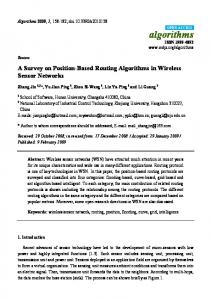
1. Introduction Automated Guided Vehicles (AGVs) are now becoming popular in automated materials handling systems, flexible manufacturing systems and even containers handling applications [see, e.g. Broadbent et al. 1985, Daniels 1988, Kim & Tanchoco 1991, 1993, Akturk & Yilmaz 1996, Yu & Huang 1997]. Figure 1 shows some commercial AGV products and their applications in different contexts. In the past decades, much research and many papers have been devoted to the technology of AGV systems, and rapid progress has been witnessed. As one of the enabling technologies, scheduling and routing of Automated Guided Vehicles (AGVs) have attracted considerable attention in the past decade [Daniels 1988, Kim & Tanchoco –1–

1991, 1993, Hsu & Huang 1994, Akturk & Yilmaz 1996, Soh et al. 1996, Yu & Huang 1997]. Many algorithms about scheduling and routing of AGVs have been proposed. However, most of the existing results are applicable to systems with small number of AGVs, offering low degree of concurrency. With drastically increased number of AGVs in recent applications (e.g. in the order of one hundred in a container terminal), efficient scheduling and routing algorithms are needed to resolve the increased contention of resources (e.g. path, loading and unloading buffers) among AGVs. Because they often employ regular route topologies, the new applications also demand innovative strategies

(a) bi-directional AGV carrying a container

(b) an AGV moving a roll of paper

(courtesy: Mentor)

(c) Left: an AGV;

(courtesy: Mentor)

Right: an AGV loading/unloading an automated cart (courtesy: TransLogic) Figure 1. Examples of AGVs

to increase system performance. In this paper, we first present descriptions of scheduling and routing of AGVs, argue that they are actually two different problems, i.e. AGV scheduling and AGV routing, although they are usually tightly associated with each other. Next, we discuss some commonly encountered phenomena when scheduling and routing AGVs. Several related problems are also compared with the problems, and therefore tailored approaches are needed to treat scheduling and routing of AGVs. We then survey the existing major works on AGV scheduling and routing and give clear –2–

classifications. Finally, we suggest that ideas of parallel processing could be adapted to schedule and route AGVs concurrently, and point out fertile areas for future study. 1.1 AGVs & AGV Systems Various papers have given different definitions for AGVs from different points of view. In brief words, an AGV is a computer-controlled, unmanned vehicle that can transport materials from point to point in a manufacturing setting [Lin 1986, Hollier 1987, Daniels 1988, Lim 1988, Goetsch 1990]. Here we adhere to the classical definition of AGVs by [MHI, 1983] as follows, which captures the key features of AGVs: An Automated Guided Vehicle (AGV) is a vehicle equipped with automatic guidance equipment, either electromagnetic or optical. Such a vehicle is capable of following prescribed guide paths and may be equipped for vehicle programming and stop selection, blocking, and any other special functions required by the system.

Figure 2. An example of an AGV system: AGVs interacting with elevators for the delivery of items throughout a building However, only when AGVs are integrated into a material handling system, referred to as the Automated Guided Vehicle System (AGVS) (Figure 2 shows an example), can

–3–

their full potentials be exploited. There also exist several alternative definitions for AGV systems. Generally, an AGV system is regarded as a material handling system in which AGVs play an important role as the main automated transportation tools [Storm 1985, Lin 1986, Hollier 1987, Daniels 1988, Lim 1988]. The following is a typical definition which captures the key elements of an AGV system [Koff 1986]: An Automated Guided Vehicle System is an automated material handling system which is controlled by a computer system and contains independently addressable driverless vehicles, i.e. the AGVs, on a predefined transportation path network. 1.2 Arising of the Problems Like a computer system, an AGV system is generally composed of two main interacting sub-systems – hardware and software. The hardware consists of the physical components, such as vehicles, path, sensors and guidance devices, controllers, etc. The software embodies approaches or algorithms for systematically managing the hardware resource of the whole AGVS so that it can work harmoniously in the highest efficiency. However, as witnessed, in the past four decades, the progress of hardware of an AGV system has been much more rapid than that of software. The lag of (controlling) software becomes an acute problem only in recent years when certain time-critical applications, e.g. container handling in seaports, involve a relatively large fleet (e.g. in the order of tens or more) of AGVs, and require a great number of tasks to be completed in real time [Soh et al. 1996, Yu & Huang 1997]. Many problems such as congestion or deadlocks in AGV operations resulting from the mismatch of software of AGV systems arise. Lying at the center of efficiency-related problems are the Scheduling and Routing of AGVs, which seemed trivial in the earlier days when the number of vehicles in an AGV system was small; they now become important and nontrivial. It was said that one of the largest port operators at Singapore has postponed its plan to deploy AGV systems in its new container port, because no satisfactory solutions to the problems of scheduling and routing of AGVs have been found so far. Therefore, there are urgent requirements both in theory and in realistic applications to discover solutions to the problems. 1.3 Organization of the Paper

–4–

The remaining sections are arranged as follows. Formal descriptions of scheduling and routing of AGVs are given in Section 2. In Section 3, we describe commonly encountered phenomena arising in scheduling and routing of AGVs. We then differentiate the problems of AGV scheduling and routing from the conventional vehicle routing problems, conventional path problems in graph theory and data routing, and argue why specialized approaches are needed for our problems. In Section 4, the existing routing algorithms are surveyed and classified. Section 5 surveys the existing scheduling algorithms. Finally, in Section 6, we give the concluding remarks and point out the directions for the future study of AGV scheduling and routing.

2. Descriptions of Issues Prior to classifying the algorithms about scheduling and routing of AGVs, it is necessary to give clear descriptions of the problems. Because of their different goals, scheduling and routing of AGVs are intrinsically two different problems, although usually they are tightly interconnected with each other. Many researchers treated them as one problem in the early years when AGV systems were relatively small in scale, because at that time they seemed trivial to some extent. However, with the increasing scale of the applications of AGV systems, the differences of these two problems become quite evident; the two problems also become nontrivial and need to be differentiated. In the following, we give verbal descriptions, as well as formulations, of the two problems. 2.1 Scheduling Briefly, the scheduling of AGVs is to dispatch a set of AGVs to complete a batch of pickup/drop-off jobs to achieve certain goals (e.g. shortest completion time, minimum AGV idle time, etc.) under given constraints. For instance, one typical scenario is to successfully achieve all the pickup/drop-off jobs under the constraints of priority or deadline. Another typical scenario is to optimize the scheduling so that the total travel time of all vehicles is minimized [Akturk & Yilmaz 1996], or the number of AGVs involved is minimized while the system throughput is as high as possible. Actually, the decision of scheduling might involve selecting a vehicle among several idling vehicles, or selecting one load among all loads

–5–

to be transported. The problem of selecting a vehicle from a pool of available vehicles is referred to as the vehicle selection or, vehicle dispatching problem. The corresponding problem of selecting a unit load among those requiring transportation is referred to as the task selection problem [Egbelu & Tanchoco 1984, Taghaboni & Tanchoco 1995]. 2.2 Routing The aim of routing AGVs is to find an optimal (e.g. shortest possible time path) and feasible route for every single AGV. The routing decision includes three aspects. Firstly, it should detect whether there exists a route which could lead the vehicle from its origin to the destination. Secondly, the route selected for an AGV must be feasible, i.e. the route must be congestion-, conflict- and deadlock-free [Taghaboni & Tanchoco 1995], etc. Thirdly, the route must be optimal or at least partially optimal, e.g. minimize idling runs of vehicles. 2.3 Formulations Here we give formal descriptions of scheduling and routing of AGVs. However, the descriptions are not unique, because different applications may emphasize different measurements or assessing criteria of an AGV system. The following are examples of problem formulations in which we emphasize the system throughput when scheduling AGVs and the total distance traveled by all AGVs when routing them. It should be easy to get similar formulations for other measurements or assessing criteria required for realistic applications of AGV systems. First, we introduce the following notations and symbols. Denote a job by an ordered pair ( ai , d i ) where ai denotes the arrival time and di the due time of the job respectively. Denote ci the completion time when job ( ai , d i ) is completed, ri the response time when the system begins to process job ( ai , d i ) . Now given a set of jobs M = { ( ai , d i ) | i = 1, 2, …, k} and n available AGVs. Our aim is to schedule the system, i.e. to assign the jobs or dispatch the vehicles, so that the system achieves the highest efficiency in term of system throughput. Assume that m is the number of AGVs scheduled to carry out all of the jobs. The problem of scheduling is hence given as follows:

–6–

minimize z =

Max( ci ) − Min( ai ) 1≤ i ≤ k

1≤ i ≤ k

k

subject to m≤n ci ≤ di , for all i = 1, 2, …, k After the scheduling plan is decided, the next step is to route AGVs so that they can get to their destinations and/or go on to carry out the other jobs. Denote si as the distance traveled by the ith AGV scheduled, the routing problem is formulated as: m

minimize z = Σ si i =1

subject to ci ≤ di , for all i = 1, 2, …, k

3. Why AGV Scheduling & Routing Require Tailored Approaches 3.1 Undesirable Circumstances in Scheduling & Routing of AGVs Although much research has been done on the problems of AGVs scheduling and routing during the past decades, there still lacks good general solutions due to the variety of applications [see, e.g. Daniels 1988, Kim & Tanchoco 1991, Soh et al. 1996, Yu & Huang 1997]. The approaches or algorithms proposed are usually only feasible for specific environments or are dealing with issues arising in particular applications. However, issues in scheduling and routing are interconnected with each other in many ways. The following listed are the commonly encountered phenomena when scheduling and routing AGVs: •

Collisions: When more than one AGV attempt to occupy the same segment of the path at the same time, clearly there will be a collision. Figure 3(a) shows two such scenarios.

•

Congestion: Congestion arises at a location where there is insufficient resource such that for a period of time the number of arrivals is greater than that of serviced requests. Figure 3(b) depicts such a case. Congestion must be reduced or eliminated because it will lower the throughput of the system or even lead to deadlocks.

–7–

•

Livelocks: As shown in Figure 3(c), a livelock may arise at the junction where the horizontal stream of traffic is given higher priority to obtain the right-of-way such that the vertical one may keep waiting indefinitely.

•

Deadlocks: A deadlock will arise when multiple AGVs mutually wait for the release (which will never occur) of the resource held by the others. Figure 3(d) shows two cases: local deadlock and non-local deadlock.

Because of their disastrous damages or negative consequences caused, all these phenomena are under the basic considerations and must be eliminated during the operations of an AGV system.

Head-to-head collision

There will be queues here

Head-to-tail collision

(a) Collisions

(b) Congestion

This queue will never move. a non-local deadlock (c) Livelock

a local deadlock

(d) Deadlocks

Figure 3. Phenomena Arising in Scheduling and Rouging of AGVs 3.2 Tailored Approaches Needed Intuitively, scheduling and routing of AGVs can be considered as one variation of the Vehicle Routing Problem (VRP) which has been approached typically by using techniques such as linear programming in operations research [Dantzig 1963, Taha 1995]. However, there are significant distinctions between them, which allow us to treat scheduling and routing of AGVs separately: •

The scale of the path networks considered in VRPs is usually metropolitan. Within a city or among cities, a vehicle can be considered as a moving point when compared with the length of the vehicle itself and the distance it travels. Whereas in an AGV

–8–

system, the distance between two depots is usually relatively short, in the order of tens of an AGV length, it is inappropriate to consider an AGV as a single point. •

With a VRP, the load capacity of a path is a consideration, collisions among vehicles are normally assumed to never occur. With an AGV system, limited by the path space, AGVs may congest or even collide with each other if the system is not well scheduled and routed.

•

With a VRP, the shortest path normally coincides with the shortest-time path (but may not be the least-cost path). With an AGV system, due to the contention of the path, it is quite common that the shortest-time path need not be the shortest path.

•

With a VRP, the path network is predefined and unchangeable. With an AGV system, sometimes the existing path layout can (or has to) be revised to yield a better scheduling or routing algorithm. It should also be pointed out that even with many advanced technological features,

the latest model of AGVs is still grossly inferior to human drivers in terms of sensory and decision-making capabilities. For example, a human driver can foresee the general “trend” of other moving vehicles and avoid congestion, either by driving around an obstacle or by taking an alternative route. In contrast, what a typical AGV possesses is only rudimentary motion primitives and collision-prevention mechanisms. As a result, much of the responsibility which previously lies on the human drivers to ensure congestion-free routing now totally lies with the software for AGV scheduling and routing. For this reason, our problems are quite different from the conventional VRPs. Therefore, appropriate and effective algorithms are always needed for an AGV system to schedule and route AGVs. The problems of scheduling and routing of AGVs are also different from the conventional path problems in graph theory, e.g. the Shortest Path Problem, Hamiltonian-Type Problem or Scheduling Problems, some of which have been proven to be NP-hard [Swamy & Thulasiraman 1981, Gondran & Minoux 1984, Wilson & Watkins 1990]. For example, a graph-theoretic problem usually cares about whether there exists an optimal path leading to a given destination node, while in an AGV system, when and how an AGV gets to its destination is also emphasized. In other words, scheduling and routing of AGVs are time-critical, while a graph-theoretic

–9–

problem usually not. This motivates us to develop tailored approaches for the scheduling and routing of AGVs. It is quite natural to also notice the similarities between the scheduling and routing of AGVs and routing data in a network. A possible analogy here is: AGVs are analogous to data packets, the paths (or tracks) to the data links, and the switching devices to the routers. However, there exist fundamental distinctions such that one scheme in a system may not be applicable directly to the other [Hsu & Huang 1994]. For example, the time for transferring electronic data packets is generally not taken as a function of physical distance between senders and receivers. While in an AGV system, the time for transporting loads is usually a function of distance between origins and destinations. Another fundamental difference is, with data routing the sender could discard and then re-send a frame of electronic data when it fails due to the congestion in the data links. In contrast, loads carried by AGVs neither have backup copies nor can be discarded. This is yet another reason for us to treat the AGV scheduling and routing as distinct problems from data routing.

4. Routing Algorithms According to the characteristics of AGV routing algorithms, the existing works could be classified into three general categories, namely, routing algorithms for general path topology, path optimization and routing algorithms for specific path topologies. Works in the first category usually treat routing problem as a graph-theoretic problem, and uses approaches such as Dijkstra’s shortest path algorithm to find optimal routes. These algorithms are usually very expensive computationally when routing more than one vehicle. By using tailored optimization techniques such as integer programming, works in the second category focus on path network optimization, in which routing control could be very simple. However, because of the heavy computation, the size of the path network to be optimized is usually small and hence only allows a small number of vehicles (at most twenty) to run on it. As for works in the third category, path networks are restricted to specific topologies such as multi-loops, and AGVs are routed and controlled by specialized algorithms.

– 10 –

4.1 Routing Algorithms for General Path Topology Algorithms in this category focus mainly on finding the feasible routes for AGVs without considering the topology characteristics of path networks. In other words, these algorithms attempt to give universal routing solutions (e.g. conflict-free shortest-time path) for general path topologies. The AGV routing problem is different from the Vehicle Routing Problem (VRP) which has been approached typically by using techniques such as linear programming or operations research [Dantzig 1963, Taha 1995]. In VRPs, vehicles will not run into collision because they are regarded as moving points when they run on the path network. However, the path for AGVs usually has limited width which may only allow no more than one AGV to run in parallel at a time. Thus, a basic consideration is to give conflict-free and shortest-time routing solutions for AGVs. The papers surveyed in the following are representative works about this issue. 4.1.1 Static routing Algorithms The concept of conflict-free shortest time AGV routing was first presented by Broadbent et al. in 1985 [Broadbent et al. 1985]. The routing procedure described in [Broadbent et al. 1985] employs Dijkstra’s shortest path algorithm to generate a matrix which describes the path occupation time of vehicles. Potential conflicts among vehicles, namely head-to-head, head-to-tail collisions and collisions at a path junction, are detected by comparing path occupation time. Then they are avoided in advance as follows: head-to-head conflicts are resolved by finding another shortest path excluding the congested segment; junction and head-to-tail conflicts are resolved by slowing the new vehicle down to let the previously scheduled vehicles proceed first. The time complexity of finding a path for a vehicle is O( N 2 ) , where N is the number of nodes (station or junction of paths) of the path network. The disadvantage of the routing procedure is that the computation could be very intensive which increases drastically with the size of the path network or the number of vehicles. Compared with uni-directional path AGV systems, there are obvious advantages of bi-directional path AGV systems in terms of utilization of vehicles and potential throughput efficiencies. Egbelu and Tanchoco showed a marked improvement in productivity and a reduction in the number of vehicles required in bi-directional path AGV systems [Egbelu & Tanchoco 1986]. The control of bi-directional path AGV – 11 –

systems can be complex because of the contention of multiple vehicles for the shared path segments. In this case, the routing algorithms must be able to eliminate potential head-to-head collisions among vehicles, and deadlocks. [Egbelu & Tanchoco 1986] first suggested the use of bi-directional path networks for routing AGVs. However, no algorithm is given to guarantee the optimality of routes for vehicles in the paper. Daniels first introduced an algorithm to route vehicles in a bi-directional flow path network, in which the partitioning shortest path (PSP) algorithm [Glover et al. 1985] is applied to find the shortest path for an AGV [Daniels 1988]. The correctness and feasibility (in terms of time/space requirements) of the algorithm was theoretically proven. The algorithm can find a conflict-free shortest-time route for a newly added AGV without changing the existing routes of the other vehicles. The computational complexity of routing a single AGV is O( N × A ) , where N represents the number of nodes and A the number of arcs in the path network (arcs are the path segments and nodes are the stations or junctions of paths). Therefore, it also suffers from high computational cost if the size of path network or the number of vehicles involved is large. In addition, when a path is allocated to a vehicle x, it is considered unusable by other newly added vehicles before x reaches its destination. In reality, the path segments of the path are only partially occupied by the vehicle during some time windows. A newly added vehicle still could run on the path segments within their free time windows. However, sometimes the algorithm may fail to find a path even if there exists one for a vehicle. In other words, the algorithm does not allow vehicles to use path resource that could otherwise be shared during different time windows. Hence the algorithm is only suitable for a system with a small path network and number of AGVs. In order to share the path segments within their free time windows, Huang et al. proposed a labeling algorithm to find a shortest time path for routing a single vehicle in a bi-directional path network [Huang et al. 1989]. The algorithm converts every arc (physical path segment) of the original path network into a node with two arcs linking with the original two nodes (these two nodes are junctions of path segments or stations). Hence a converted network is obtained and then labels are assigned to free time windows defined for each node. By comparing the labels of every node, a shortest time path could be obtained if it exists. The algorithm has the time complexity of O( D 2 log D ) for a single vehicle, where D is the total number of time windows of all

– 12 –

nodes in the converted network. The main disadvantage of the algorithm is the unacceptably large amount of computation. The converted network has double number of arcs and at least double number of nodes than the original network (because in a connected graph, the node number N and the arc number A satisfy A ≥ N − 1 ), and every node has at least one time window. Therefore the information of network could require a lot of memory space. The actual time complexity for a single vehicle is O(( N + A )2 log( N + A )) , where N and A represent the numbers of nodes and arcs in the original path network respectively. Kim and Tanchoco also presented a conflict-free shortest-time algorithm for routing AGVs in a bi-directional path network [Kim & Tanchoco 1991]. The proposed algorithm is based on Dijkstra’s shortest-path algorithm. It maintains, for each node, a list of time windows reserved by scheduled vehicles and a list of free time windows available for vehicles to be scheduled. The concept of time window graph is introduced, in which the node set represents the free time windows and the arc set represents the reachability among free time windows. Then the algorithm routes vehicles through the free time windows of the time window graph instead of the physical nodes of the path network. To get an optimal routing solution, the algorithm could take a large amount of time. Specifically, it requires O( v 4 n 2 ) computations in the worst case, where v is the number of vehicles and n is the number of nodes. Therefore, it will be more suitable for a small system with a few vehicles. Kim and Tanchoco later gave the operational control of bi-dirctional path network AGV systems for the conflict-free shortest-time routing algorithm [Kim & Tanchoco 1993]. The research employs a conservative myopic strategy, in which only one vehicle is considered at a time and all the previous decisions are strictly respected and a subsequent travel schedule is assigned only after the vehicle becomes idle. Using this strategy, to find a path from the current position of a vehicle to a pickup station and then to the drop-off station, the system controller need only call at most twice the conflictfree shortest-time routing algorithm described in [Kim & Tanchoco 1991] after the decision on vehicle dispatching is made. 4.1.2 Dynamic Routing Algorithms The preceding algorithms are static and global routing methods, which generally take a relatively long time to compute an optimal route. To speed up the processes of finding – 13 –

optimal or feasible routes for AGVs, dynamic routing techniques and algorithms are proposed. Taghaboni and Tanchoco proposed a dynamic routing technique, namely incremental route planning, which can route AGVs relatively quickly [Taghaboni & Tanchoco 1995]. The algorithm selects the next node for the vehicle to visit so as to reach its destination based on the status of neighbouring nodes and information about the global network. The next node is selected among all adjacent nodes such that it will result in the shortest travel time. The decision of next node selection is repeated until the vehicle reaches its destination. The algorithm can work in both uni-directional and bidirectional path networks. However, compared with the complete route planner [Taghaboni & Tanchoco 1995], the incremental route planning can not achieve a high efficiency when the number of tasks and vehicles increase. The algorithm may also not obtain an optimal route and correctly predict the delays in some cases. Based on dynamic programming, Langevin et al. presented an algorithm which could give an optimal integrated solution for planning the dispatching, conflict-free routing, and scheduling of AGVs in a flexible manufacturing system [Langevin et al. 1996]. The algorithm defines a partial transportation plan as a schedule and a route for each vehicle satisfying a subset of the transporation tasks. States are defined corresponding to the partial transportation plans. The dynamic programming operations work on the states to find the best final state set which contains the optimal solution. However, as stated in the study, the number of states could be astronomical for a large system. To make it usable, a procedure is designed to elimiate some of the states. Even so, the computation can be very expensive. And the fatal limitation is that the algorithm only considers the system with two vehicles, although the path network may be bidirectional. Therefore, the throughput of such a system may not scale up with the number of tasks. An extended version of the algorithm is also given in the study to deal with the system with more than two vehicles. However, it still cannot guarantee the optimality of the solutions. Table 1 and Table 2 summarize this part of work. 4.2 Path Optimization Due to the large amount of computation for finding the optimal routes in a general path network, many researchers propose the idea of tailoring the path network to achieve a

– 14 –

higher efficiency. This part of work emphasizes on the optimization of path layout rather than routing algorithms with consideration of the given facility and pickup/dropoff stations (or P/D stations for short). This optimization problem is usually formulated in integer programming models. 4.2.1 0-1 Integer Programming Models Gaskins and Tanchoco first formulated the path layout problem as a zero-one integer programming model with consideration of the given facility layout and pickup/drop-off stations [Gaskins & Tanchoco 1987]. The objective is to find an optimal path network which will minimize total traveling distance of loaded vehicles. However, the paper only considers uni-directional path network, which has lower utilization [Egbelu & Tanchoco 1986]. The distance traveled by unloaded vehicles is not taken into considerations, which may affect the routing control and system throughput. The main limitation of the study is that it only considers a fleet of AGVs with the same origin and destination every time. These AGVs run along the same route. Therefore, in this case routing control is trivialized since issues such as congestion, deadlocks and conflicts, will never arise. Because routing control is not taken into account, when AGVs with different origins and destinations run simultaneously, conflicts may occur among them. Another limitation from the formulated zero-one integer programming model is that it has a very low probability to obtain a non-empty solution set. Moreover, for practical problems, the number of zero-one variables tends to be very large and computational efficiency becomes a critical issue. Based on a zero-one integer programming model and the branch-and-bound method, Kaspi and Tanchoco proposed an alternative formulation [Kaspi & Tanchoco 1990] of the AGV path layout problem described in [Gaskins & Tanchoco 1987]. The new approach can obtain the best path design provided that the pickup/drop-off stations location and facility layout are given. The procedure, compared with the algorithm in [Gaskins & Tanchoco 1987], reduces the computation time at the cost of the quality of path design because not all of the possibilities are enumerated. However, this study shares the same limitation with the previous one. 4.2.2 Intersection Graph Method An Intersection Graph Method (IGM) is presented by [Sinriech & Tanchoco 1991] for solving AGV Flow Path Optimization Model developed by [Kaspi & Tanchoco 1990]. – 15 –

A procedure based on the technique of branch-and-bound is described wherein only a reduced subset of all nodes in the path network is considered. Only intersection nodes are used to find optimal solutions. With this improved procedure, the number of branches of the main problem is only half of that of the method described in [Kaspi & Tanchoco 1990]. The amount of computation is thus greatly reduced. Therefore, this approach could be adopted by a relatively large AGV system. However, because only intersection nodes in path are used, the algorithm might miss some optimal solutions. The same problem is also studied by Goetz and Egbelu in a different approach [Goetz & Egbelu 1990]. They modeled and solved the problem of selecting the guide path as well as the location of the pickup and drop-off stations as an integer linear program. The objective is to minimize the total distance traveled by both loaded and unloaded AGVs. A heuristic algorithm is used in the study to reduce the size of the problem. The reduction makes the approach more amenable for use in the design of large path layouts. Then the problem of determining the optimal locations of the pickup/drop-off stations is formulated based on the reduced problem. The paper also exploits the structure of the problem to reduce the number of constraints required to solve the path layout problem. However, the issues of vehicle number that the system could have and the routing control on the optimized path network are not considered in the study, which are obviously related to the final goal of the system optimization. The path studied here is uni-directional, which, to some extent, results in a low path utilization and system throughput. Table 3 summarizes the works reviewed in the preceding paragraphs. 4.3 Routing Algorithms for Specific Path Topologies Some algorithms are proposed for routing AGVs in specific path topologies, such as single-loop, multi-loops, and mesh. 4.3.1 Closed Single-loop Tanchoco and Sinriech suggested an optimal closed single-loop path layout for an AGV system [Tanchoco & Sinriech 1992]. An algorithm based on integer programming is given to find the optimal single loop. With the single-loop path layout, the routing algorithm could be very straightforward. In this case, if all vehicles run in the same direction with uniform speed, no collisions may occur among them because there are no

– 16 –

intersections in the optimal singe loop path. As the paper claims, however, the system throughput drops down a little compared with general path systems. It allows at most ten vehicles to run simultaneously around the single loop [Tanchoco & Sinriech 1992]. Therefore, such an AGV system could not be very suitable for a large material handling system with a relatively great number of vehicles and stations. 4.3.2 Non-overlapping Closed Loops Lin and Dgen provided an algorithm for routing AGVs among non-overlapping closed loops within a tandem AGV system [Lin & Dgen 1994]. Stations within each loop are served by a single dedicated vehicle. The transit area located between two adjacent loops serves as an interface and allows loads to be transferred from one loop to another. If a load needs to be delivered to a station not located within the same loop, the load needs more than one vehicle to carry it to its destination. A task-list time-window algorithm is employed to find a shortest travel time path based on the current status to route a vehicle from point A to point B. The computation for a routing decision is relatively small. However, since only one vehicle serves a loop, the throughput of the system is very low. Besides, the device used to transfer loads from one loop to another usually increases the system cost. Therefore, the scale of such a system could not be very large. The paper did not address the design issue of the loops, which is crucially related to the system efficiency. 4.3.3 Segmented Flow Topology Similar to the multi-loops path layout in [Lin & Dgen 1994], Sinriech and Tanchoco proposed an alternative path topology – Segmented Flow Topology (SFT) [Sinriech & Tanchoco 1994]. The SFT can be used in conjunction with each of the following three network types: connected, partitioned and split-flow. The general SFT is comprised of one or more zones, each of which is separated into non-overlapping segments with each segment serviced by a single vehicle. Transfer buffers are located at both ends of every segment. Since there is only one vehicle moving in a segment, no path segment contentions will occur. The vehicle can move bi-directionally in the segment. Therefore, the routing control for such a path topology is very simple. The advantage of the SFT can be easily recognized by the lower value of flow × dis tan ce compared with that of the other path topologies, such as single-loop, bi-directional and uni-directional conventional paths, etc. However, the transferring devices in the buffers are the – 17 –

additional cost of the overall system. The operations of transferring loads among segments may be time-consuming and sometimes cause delay of transportation. 4.3.4 Linear Array, H-tree, 2D-mesh etc. Hsu and Huang gave time and space complexities for some basic AGV routing operations in several specific bi-directional path topologies [Hsu & Huang 1994, Huang & Hsu 1994]. The routing operations include simple delivery, distribution, scattering, accumulation, gathering, sorting and total exchange. All these operations are achieved in the following path topologies: linear array, ring, H-tree, star, 2D-mesh, n-cube and cube-connected cycles and complete graph. The upper bounds of time and space complexities for those AGV routing in those path topologies are Θ( n 2 ) and Θ( n 3 ) respectively, where n is the number of nodes in the path topologies. However, the paper does not give in detail the routing algorithms and the techniques to avoid congestion, conflicts, deadlocks etc. It also causes additional system cost if every node in the path network has an arbitration capability. Table 4 summarizes this part of work.

5. Scheduling Algorithms The AGV systems considered above usually have a relatively small number of vehicles and P/D jobs. In this case, the problem of AGV scheduling is trivial with the existing solutions of path network optimization and routing control. However, for an AGV system with a great number of P/D jobs and a large size of AGV fleet, such as container handling in a seaport, the scheduling of AGVs becomes nontrivial. It should be studied separately from routing problem and path layout design. However, recent research on AGV scheduling is relatively scarce and limited in scope. A typical work on AGV scheduling is by Akturk and Yilmaz in 1996. They proposed an algorithm to schedule vehicles and jobs in a decision-making hierarchy based on the mixed integer programming [Akturk & Yilmaz 1996]. The proposed micro-opportunistic scheduling algorithm (MOSA) combines two perspectives, namely job-based and vehicle-based approaches, into a single algorithm in which both the critical jobs and the travel time of unloaded vehicles are considered simultaneously. The scheduling problem is defined similarly to, but not identically as, the Time Constrained Vehicle Routing Problem (TCVRP) which is proven to be NP-hard by [Kolen et al.

– 18 –

1987]. The problem is thus solvable in polynomial time because the objective is to minimize the deviation of the time windows rather than the distance traveled by vehicles in TCVRP. However, the MOSA is only applicable for AGV systems with a small number of jobs and vehicles. This is because with the increase of job number and the size of vehicle fleet, the amount of computation for the solution could become unacceptably large. Qiu and Hsu presented a scheme to schedule and route AGVs on a bi-directional linear path layout [Qiu & Hsu 1999, 2000]. The proposed algorithm actually combines the functions of scheduling and routing, and employs the idea of concurrent processing. When AGVs are scheduled and routed to run along the linear tracks, no conflicts, congestion, livelocks or deadlocks will arise. All jobs can be completed within a very short time. The efficiency of the algorithm is not constrained by the size of the system. Because the algorithm is given based on the designed linear path layout, it can be classified into the category of routing (and scheduling) algorithms for specific path topologies. However, how to schedule and route pickup/drop-off jobs continuously is still unsolved in the paper. Moreover, the stringent (and unrealistic) synchronization requirements of vehicles should be relaxed to meet realistic applications. Kim and Bae presented a model for scheduling AGVs for multiple container cranes [Kim & Bae 1999]. The primary objective is to minimize the delay of carrying out all loading and unloading operations. In other words, the goal is to minimize the waiting time of container cranes rather than to minimize the idle running of AGVs. Issues related to AGV routing are not taken into considerations. Hence with the increase of the number of AGVs, congestion or even collisions of AGVs might occur at the operating area of container cranes.

6. Future Directions & Concluding Remarks For future research, we believe that the most promising area is in the development of new AGV routing algorithms for specific path topologies: •

In many applications, the AGV path networks are regular graphs, e.g. linear array, loop/loops, 2D-mesh. For example, in a container handling application, the container stacking yards are usually arranged as rectangular areas connected with mesh-like paths. – 19 –

•

Routing algorithms for specific path topologies usually have relatively lower computational complexity compared with those for general path topology.

•

Developing routing algorithms for specific path topologies is relatively more feasible than those for general path topology. Meanwhile, because we can exploit the characteristics of these specific topologies, we could develop algorithms that are more efficient.

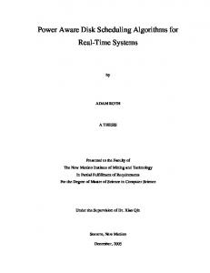
AGV scheduling should be treated as a different problem from AGV routing. However, we cannot disregard its association with routing when developing scheduling algorithms. One of the feasible and possibly effective ways is to combine the functions of scheduling and routing into one algorithm, as the algorithm presented by Qiu and Hsu.10,11 Another way is to first give a scheduling plan and then develop suitable routing algorithm for it. Another strategy is to study scheduling algorithms based on a given routing algorithm. In spite of the pervasive applications of AGV systems, the problems of scheduling and routing of AGVs still call for much attention to. Even in the latest conferences on robotics and intelligent vehicles, e.g. the 1999 International Conference on Field and Service Robotics38 and 1999 Symposium on Intelligent Transportation Systems,39 much study focuses on the difficult issues such as automated driving of vehicles, intelligentization of vehicles, intelligent navigation mechanisms, robot vision, image processing, information fusion, etc. Relatively fewer papers refer to scheduling and routing of AGVs. It should be pointed out that even if issues on vehicle automation or intelligentization are fully resolved, this does not mean that the problems of scheduling and routing will disappear accordingly. Without suitable algorithms of scheduling and routing, no one can guarantee that congestion or deadlocks will not occur even if all vehicles are driven by human drivers. On the other hand, with good scheduling and routing algorithms, based on the current level of AGV technologies, an AGV system could be put into operation before the difficult issues mentioned above are resolved. As a case in point, presently at Nanyang Technological University, Singapore, a project of AGV application in a container handling system is being studied.40 The main goal is to schedule and route AGVs within a mesh-like path and container stacking areas (as shown in Figure 4). The solutions to the problems could greatly decrease the system costs because in this case AGVs may not require too much intelligence.

– 20 –

In conclusion, it should be clear that AGV systems are, intrinsically, parallel and distributed systems that require a high degree of concurrency. We feel that the routing and scheduling of these systems should be a fertile area where computer scientists and engineers can have significant impacts and contributions.

Bi-directional paths

An AGV is loading

Buffers in yard areas for AGVs loading or unloading

An AGV is loading/unloading at a container crane Container cranes

Free AGVs are running to their origins to load

A loaded AGV is running to its destination

A container ship

An AGV is unloading

Containers stacking in yard areas (different colors represent different stacking heights of containers) Figure 4. AGVs in a mesh-like path and container stacking areas

– 21 –

Table 1 Static Routing Algorithms for General Path Topology

Computational Complexity Path Direction

Broadbent et al. 1985 Finding conflictfree shortest time routes for AGVs Dijkstra’s shortest path algorithm O( N 2 ) (average case) Bi-directional

Advantages

Easy to execute

Problems Solved Basic Algorithms

Disadvantages

Daniels 1988

Huang et al. 1989

Finding conflict-free shortest time routes for AGVs Partitioning shortest path algorithm

Finding conflict-free shortest time routes for AGVs

O( N × A ) (average case)

O(( N + A )2 log( N + A )) (average case) Bi-directional Time windows are used for every node; the utilization of path segments are increased Heavy computation; large amount of data of converted network to maintain

Bi-directional Easy to execute and faster than Broadbent’s

Heavy Heavy computation; low computation; low utilization of path utilization of segments; may cause path segments failure in finding routes that actually exist

–

Kim & Tanchoco 1991, 1993 Finding conflict-free shortest time routes for AGVs Dijkstra’s shortest path algorithm; conservative myopic strategy O( v 4 N 2 ) (worst case) Bi-directional Easy to execute and control; fast

Heavy computation; large amount of data of path network to maintain

Legend: N – node number in the path network; A – arc number in the path network; v – vehicle number;

– 22 –

Table 2 Dynamic Routing Algorithms for General Path Topology

Problems Solved Basic Algorithms Optimality of Solutions Path direction Advantages Disadvantages

Taghaboni & Tanchoco 1995 Finding a conflict-free route for AGVs

Langevin et al. 1996 Integrated solution for AGV dispatching, conflict-free routing and scheduling Incremental route planning Dynamic programming Not guaranteed Not guaranteed Bi-directional & Uni-directional Bi-directional Relatively fast in routing decision Easy to execute and control Low efficiency when the numbers of tasks and Since only two vehicles are allowed in the system, the system throughput and vehicles increase; also no optimal routing path utilization could be very low; only solutions could be guaranteed; suitable for very small system with a few stations

– 23 –

Table 3 Path Optimization Gaskins & Tanchoco 1987

Kaspi & Tanchoco 1990

Advantages

Disadvantages

– 24 –

Goetz & Egbelu 1990

1991

Path optimization to Path optimization to minimize total distance minimize total traveled by loaded distance traveled by vehicles loaded vehicles Intersection Graph Zero-one integer Method; programming; Branch-and-bound branch-and bound General General General Uni-directional Uni-directional Uni-directional An improved model of An improvement of Very easy to that proposed in [Kaspi & the approach in implement for a fleet [Gaskins & Tanchoco Tanchoco 1990]; reduced of AGVs with the number of problem 1987]; reduced same origins and computation; branches; optimality destinations; guaranteed optimality guaranteed Conflicts may occur Distance traveled by Only intersection nodes of when there are AGVs unloaded AGVs is not the path network are with different origins considered; low considered; optimal and destinations; heavy system throughput; solutions may be missed computation; low still heavy system throughput computation

Path optimization to Problems Solved minimize total distance traveled by loaded vehicles Zero-one integer Basic Algorithms programming Path Topologies Path Direction

Sinriech & Tanchoco

Path optimization to minimize total distance traveled by both loaded and unloaded vehicles Integer linear programming General Uni-directional Problem size is reduced; distance traveled by unloaded vehicles is considered together; optimality is hence better ensured Routing control and vehicle number are not considered in the study which are important for AGV systems

Table 4 Algorithms for Specific Path Topologies (to be continued)

Problems Solved Basic Algorithms

Tanchoco &Sinriech 1992 Optimizing the path layout configuration in a closed single loop Integer programming

Lin & Dgen 1994 Routing AGVs among several non-overlapping closed loops; finding shortest travel time path The task-list time-window algorithm

Sinriech & Tanchoco 1994 Routing AGVs among several non-overlapping path segments; finding shortest travel time path –

Path Topologies

Closed single-loop

Multi-loop

Segmented path topology

Path Direction

Uni-directional

Bi-directional or Unidirectional

Bi-directional or Unidirectional

– 25 –

Hsu & Huang 1994 Route planning for basic routing functions on several specific basic path topologies – Linear array, ring, H-tree, star, 2D-mesh, n-cube, cube-connected cycles, complete graph, Bi-directional

Table 4 Algorithms for Specific Path Topologies (continued)

Advantages

Disadvantages

Tanchoco &Sinriech 1992 Routing control is very easy; no conflicts or deadlocks will occur; easy for implementation Low system throughput ; only suitable for small system

Lin & Dgen 1994 Easy for routing control since every loop is served by a single vehicle;

Low system throughput; additional cost needed for transit device between two adjacent loops; indirect transportation may cause delay

– 26 –

Sinriech & Tanchoco 1994 An alternative design of that in [Lin & Dgen 1994]; relatively low value of flow×distance

Low system throughput with one vehicle serving in a segment; additional cost for transit device; indirect transportation may cause delay

Hsu & Huang 1994 Give the time and space complexities for basic routing functions which are upper- bounded by Θ( n 2 ) and Θ( n 3 ) respectively Routing control not given in detail; the assumption of arbitration capability for every buffer is too idealized

7. References 1. Akturk, M. S. and Yilmaz, H., 1996, Scheduling of Automated Guided Vehicles in a Decision-Making Hierarchy. Int’lJof Production Research, 34(2), 577-591. 2. Broadbent, A. J., Besant, C. B., Premi, S. K., and Walker,S. P. 1985, Free ranging AGV Systems: Promises, Problems and Pathways. Proc. of the 2nd Int’l Conf. on Automated Materials Handling, (IFS Publication Ltd., UK), pp. 221-237. 3. Daniels, S. C., 1988, Real-time Conflict Resolution in Automated Guided Vehicle Scheduling. Ph.D. thesis, Dept. of Industrial Eng., Penn. State University, USA. 4. Dantzig, G., 1963, Linear Programming and Extensions. Princeton University Press, Princeton, N.J. 5. Egbelu, P. J. and Tanchoco, J. M. A., 1984, Characterization of Automatic Guided Vehicle Dispatching Rules. Int’l J. of Production Research, 22(3), 359-374. 6. Egbelu, P. J. and Tanchoco, J. M. A., 1986, Potentials for Bidirectional Guidepath for Automatic Guided Vehicle Systems. Int’l J. of Prod. Res., 24(5), 1075-1097. 7. Gaskins, R. J. and Tanchoco, J. M. A., 1987, Flow Path Design for Automated Guided Vehicle Systems. Int’l J. of Production Research, 25(5), 667-676. 8. Glover, F., Klingman, D. D. and Phillips, N. V., 1985, A New Polynomially Bounded Shortest Path Algorithm. Operations Research, 33(1) 65-73. 9. Goetsch, D.L., 1990, Advanced Manufacturing Technology. Delmar Publishers Inc. 10. Goetz, W. G. and Egbelu, P. J., 1990, Guide Path Design and Location of Load Pick-up/drop-off Points for an Automated Guided Vehicle System. Int’l J. of Production Research, 28(5), 927-941. 11. Gondran, M. and Minoux, M., 1984, Chapter 2, 8, 10,11, Graphs and Algorithms. A Wiley-Interscience Publication, John Wiley & Sons, Inc. 12. Hollier, R. H., 1987, Automated Guided Vehicle Systems. IFS (Publications) Ltd., UK and Springer-Verlag. 13. Hsu, W. J. and Huang, S. Y., 1994, Route Planning of Automated Guided Vehicles. Proc. of Intelligent Vehicles, Paris, 479-485. 14. Huang, J., Palekar, U. S. and Kapoor, S. G., 1989, A Labeling Algorithm for the Navigation of Automated Guided Vehicles. Advances in Manu. Systems Eng., Proc. of the ASME Winter Annual Meeting, San Francisco, CA, PED-Vol. 37, 181-193.

– 27 –

15. Huang, S. Y. and Hsu, W. J., 1994, Routing Automated Guided Vehicles on MeshLike Topologies. Int’l Conf. on Automation, Robotics and Computer Vision. 16. Kaspi, M. and Tanchoco, J. M. A., 1990, Optimal Flow Path Design of Unidirectional AGV Systems. Int’l J. of Production Research, 28(6), 915-926. 17. Kim, C. W. and Tanchoco, J. M. A., 1991, Conflict-free Shortest-time Bi-directional AGV Routing. Int’l J. of Production Research, 29(12), 2377-2391. 18. Kim, C. W. and Tanchoco, J. M. A., 1993, Operational Control of a Bi-directional Automated Guided Vehicle Systems. Int’l J. of Production Res., 31(9), 2123-2138. 19. Kim, K. H. and Bae, J. W., 1999, Dispatching Automated Guided Vehicles for Multiple Container-Cranes. Seminar on Port Design and Operations Technology, Pan Pacific Hotel, Singapore, 4-5 Nov 1999. 20. Koff, G. A., 1986, Basis of AGVS. SME ULTRATECH, Vol. 1, Conference Procedings, September. 3.1-3.17. 21. Kolen, A. W. J., Rinnooy-Kan, A. H. G. and Trienekens, H. W. J. M., 1987, Vehicle Routing with Time Windows. Operations Research, 35(2), 266-274. 22. Langevin, A., Lauzon, D. and Riopel, D., 1996, Dispatching, Routing and Scheduling of Two Automated Guided Vehicles in a Flexible Manufacturing System. Int’l J. of Flexible Manufacturing System, 8(1996): 246-262. 23. Lin, J. T., 1986, Development of a Graphic Simulation Model for Design of Automated Guided Vehicle Systems. Ph.D. thesis, Department of Industrial Engineering, Lehigh University, USA. 24. Lin, J. T. and Dgen, P.-K., 1994, An Algorithm for Routing Control of a Tandem Automated Guided Vehicle System. Int’l J. of Production Res., 32(12), 2735-2750. 25. Material Handling Institute, 1983. Considerations for Planning and Installing Automated Guided Vehicle Systems. 26. Proceedings of the International Conference on Field and Service Robotics, August 29-31, 1999, Pittsburgh, Pennsylvania, USA. 27. Qiu, L. and Hsu, W. J., 1999, Scheduling and Routing of AGVs on a Linear Path Layout. Technical Report: CAIS-TR-99-27, Centre for Advanced Information Systems, School of Applied Science, Nanyang Technological University, Singapore, Oct 1999. Also available at http://www.cais.edu.sg:8000/.

– 28 –

28. Qiu, L. and Hsu, W. J., 2000, Conflict-free AGVs Routing in a Linear Path Layout. Accepted for the 5th Int’l Conf. on Computer Integrated Manufacturing, Singapore, March 2000. 29. Soh, J. T. L., Hsu, W. J., Huang, S. Y. and Ong, A. C. Y., 1996, Decentralized Routing Algorithms for Automated Guided Vehicles. Proc. of ACM Symposium of Applied Computing, 473-479. 30. Sinriech, D. and Tanchoco, J. M. A., 1991, Intersection Graph Method for AGV Flow Path Design. Int’l J. of Production Research, 29(9), 1725-1732. 31. Sinriech, D. and Tanchoco, J. M. A., 1994, SFT – Segmented Flow Topology. In Material Flow Systems in Manufacturing, chapter 8, J. M. A. Tanchoco (ed.), London: Chapman & Hall, pp. 200-235. 32. Storm, J. O., 1985, The Role of AGVS in an FMS Environment. Proc. of Sessions VII and X, ProMat 85, MHI, February 25-28. 33. Swamy, M. N. S. and Thulasiraman, K., 1981, Chapter 3, 15, Graphs, Networks, and Algorithms. A Wiley-Interscience Publication, John Wiley & Sons, Inc. 34. Symposium on Intellegent Transportation Systems. Nov 29-30, 1999, Singapore. Also available at http://www.inrialpes.fr/sharp/SITS.99/. 35. Taghaboni, F. and Tanchoco, J. M. A., 1995, Comparison of Dynamic Routing Techniques for Automated Guided Vehicle Systems. Int’l J. of Production Research, 33(10), 2653-2669. 36. Taha, H. A., 1995, Operations Research, an Introduction. Prentice Hall Int’l, Inc., Simon & Schuster (Asia) Pte. Ltd., Singapore, fifth edition. 37. Tanchoco, J. M. A. and Sinriech, D., 1992, OSL-Optimal Single-Loop Guided Paths for AGVS. Int’l J. of Production Research, 30(3), 665-681. 38. Vee, V. Y., Ye, R., Shah, S. N. and Hsu, W. J., 1999, Meeting Challenges of Container Port Operations for Next Millennium. Technical Report: CAIS-TR-99-25, Centre for Advanced Information Systems, School of Applied Science, Nanyang Technological University, Singapore. Available at http://www.cais.edu.sg:8000/. 39. Wilson, R. J. and Watkins, J. J., 1990, Chapter 8, 9, Graphs: an Introductory Approach. John Wiley & Sons, Inc. 40. Yu, X. and Huang, S. Y., 1997, A Centralized Routing Algorithm for AGVs in Container Ports. Proc. of 4th Int’l Conf. on Computer Integrated Manu., pp 589-600.

– 29 –