Scheduling Contention-Free Irregular Redistributions in Parallelizing Compilers Chao-Yang Lan, Ching-Hsien Hsu and Shih-Chang Chen Department of Computer Science and Information Engineering Chung Hua University, Hsinchu, Taiwan 300, R.O.C. Email:
[email protected] Abstract. Many scientific problems have been solved on distributed memory multi-computers. For solving those problems, efficient data redistribution algorithm is necessary. Irregular array redistribution has been paid attention recently since it can distribute different size of data segment to processors according to their own computation ability. It’s also the reason why it has been kept an eye on load balance. High Performance Fortran Version 2 (HPF2) provides GEN_BLOCK (generalized block) distribution format which facilitates generalized block distributions. In this paper, we present a two-phase degree-reduction (TPDR) method for scheduling HPF2 irregular array redistribution. In a bipartite graph representation, the first phase schedules communications of processors that with degree greater than two. Every communication step will be scheduled after a degree-reduction iteration. The second phase schedules all messages of processors that with degree-2 and degree-1 using an adjustable coloring mechanism. An extended algorithm based on TPDR is also presented in this paper. Effectiveness of the proposed methods not only avoids node contention but also shortens the overall communication length. To evaluate the performance of our methods, we have implemented both algorithms along with the divide-and-conquer algorithm. The simulation results show improvement of communication costs. The proposed methods are also practicable due to their low algorithmic complexity. Keywords: Irregular redistribution, communication scheduling, GEN_BLOCK, degree-reduction
1. Introduction Parallel computing systems have been used to solve complex scientific problems using their powerful computational ability. Dealing with those kinds of problems, systems must process large number of data. For this reason, keeping load balancing is important. In order to achieve a good performance of load balancing, using an appropriate data distribution scheme [8] when processing different phase of application is necessary. In general, data distribution can be classified into regular and irregular. The regular distribution usually employs BLOCK, CYCLIC, or BLOCK-CYCLIC(c) to specify array decomposition. The irregular distribution uses user-defined functions to specify unevenly array distribution. To map unequal sized continuous segments of array onto processors, High Performance Fortran version 2 (HPF2) provides GEN_BLOCK distribution format which facilitates generalized block distributions. GEN_BLOCK allows unequal sized data segments of an array to be mapped onto processors. This makes it possible to let different processors dealing with appropriate data quantity according to their computation ability. In some algorithms, an array distribution that is well-suited for one phase may not be good for a subsequent phase in terms of performance. Array redistribution is needed when applications running from one sub-algorithm to another during run-time [6]. Therefore, many data parallel programming languages
support run-time primitives for changing a program’s array decomposition. Since array redistribution is performed at run-time, there is a performance trade-off between the efficiency of the new data decomposition for a subsequent phase of an algorithm and the cost of redistributing array among processors. Thus efficient methods for performing array redistribution are of great importance for the development of distributed memory compilers for those languages. Communication scheduling is one of the most important issues on developing runtime array redistribution techniques. In this paper, we present a two-phase degree reduction (TPDR) algorithm to efficiently perform GEN_BLOCK array redistribution. Degree here means the maximum number between in-degree and out-degree among all vertices in a bipartite graph as presented in figure 1. The main idea of the two-phase degree reduction method is to schedule communications of processors that with degree greater than two in the first phase (degree reduction phase). Every communication step will be scheduled after a degree-reduction iteration. The second phase (coloring phase) schedules all messages of processors that with degree-2 and degree-1 using an adjustable coloring mechanism. Based on the TPDR method, we also present an extended TPDR algorithm (E-TPDR). The proposed techniques have the following characteristics: z z
It is a simple method with low algorithmic complexity to perform GEN_BLOCK array redistribution. The two-phase degree reduction technique can avoid node contentions while performing irregular
array redistribution. The two-phase degree reduction method is a single pass scheduling technique. It does not need to re-schedule / re-allocate messages. Therefore, it is applicable to different processor groups without increasing the scheduling complexity. The rest of this paper is organized as follows. In Section 2, a brief survey of related work will be presented. In section 3, we will introduce an example of GEN_BLOCK array redistribution as preliminary. Section 4 presents two communication scheduling algorithms for irregular redistribution problem. The performance analysis and simulation results will be presented in section 5. Finally, the conclusions will be given in section 6. z
2. Related Work Many methods for performing array redistribution have been presented in the literature. These researches are usually developed for regular or irregular problems [5] in multi-computer compiler techniques or runtime support techniques. We briefly describe the related works in these two aspects. Techniques for regular array redistribution, in general, can be classified into two approaches: the communication sets identification techniques and communication optimizations. The former includes the PITFALLS [17] and the ScaLAPACK [16] methods for index sets generation; Park et al. [14] devised algorithms for BLOCK-CYCLIC Data redistribution between processor sets; Dongarra et al. [15] proposed algorithmic redistribution methods for BLOCK-CYCLIC decompositions; Zapata et al. [1] proposed parallel sparse redistribution code for BLOCK-CYCLIC data redistribution based on CRS structure. The Generalized Basic-Cycle Calculation method was presented in [3]. Techniques for communication optimizations category, in general, provide different approaches to reduce the communication overheads in a redistribution operation. Examples are the processor mapping techniques [10, 12, 4] for minimizing data transmission overheads, the multiphase redistribution strategy [11] for reducing message startup cost, the communication scheduling approaches [2, 7, 13, 21] for avoiding node contention and the strip mining approach [18] for overlapping communication and computational overheads. On irregular array redistribution, some work has concentrated on the indexing and message generation while some has addressed on the communication efficiency. Guo et al. [9] presented a symbolic analysis method for communication set generation and to reduce communication cost of irregular array redistribution. On communication efficiency, Lee et al. [12] presented a logical processor reordering algorithm on irregular array redistribution. Four algorithms were discussed in this work for reducing communication cost. Guo et al.
[19, 20] proposed a divide-and-conquer algorithm for performing irregular array redistribution. In this method, communication messages are first divided into groups using Neighbor Message Set (NMS), messages have the same sender or receiver; the communication steps will be scheduled after those NMSs are merged according to the relationship of contention. In [21], a relocation algorithm was proposed by Yook and Park. The relocation algorithm consists of two scheduling phases, the list scheduling phase and the relocation phase. The list scheduling phase sorts global messages and allocates them into communication steps in decreasing order. Because of conventional sorting operation, list scheduling indeed performs well in term of algorithmic complexity. If a contention happened, the relocation phase will perform a serial of re-schedule operations. While algorithm flow goes to the relocation phase, it has to allocate an appropriate location for the messages that can’t be scheduled at that moment. This leads to high scheduling overheads and degrades the performance of a redistribution algorithm.
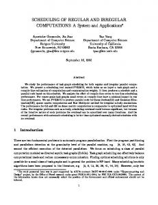
3. GEN_BLOCK Array Redistribution In this section, we will present some properties of irregular array redistribution. To simplify the presentation, notations and terminologies used in this paper are prior defined as follows. Definition 1: Given an irregular GEN_BLOCK redistribution on a one-dimension array A[1:N] over P processors, the source processors of array elements A[1:N] is denoted as SPi; the destination processors of array elements A[1:N] is denoted as DPi where 0 ≤ i ≤ P−1. Definition 2: A bipartite graph G = (V, E) is used to represent the communications of an irregular array redistribution on A[1:N] over P processors. Vertices of G are used to represent the source and destination processors. Edge eij in G denotes the message sent from SPi to DPj, where eij ∈ E. |E| is given as the total number of communication messages through the redistribution. Figure 1(a) shows an example of redistributing two GEN_BLOCK distributions on an array A[1:100]. Distributions I and II are mapped to source processors and destination processors, respectively. The communications between source and destination processor sets are depicted in Figure 1(b). There are totally eleven communication messages (|E|=11), m1, m2, m3…, m11 among processors involved in the redistribution. In general, to avoid conflict communication or node contention, a processor can only send one message to destination processors at a communication step. Similarly, one can only receive a message from source processors at any communication step. In other words, messages sent or received by the same processor can’t be scheduled in the same communication step. The messages which can not be scheduled in the same communication step are called
conflict tuple [19]. For instance, {m1, m2} is a conflict tuple since they have common destination processor DP0; {m2, m3} is also a conflict tuple because of the common source processor SP1. Figure 1(c) shows a simple schedule for this example. Unlike regular problem, there is no repetition communication pattern in irregular GEN_BLOCK array redistribution. It is also noticed that if SPi sends messages to DPj-1 and DPj+1, the communication between SPi and DPj must exist, where 0≤ i, j ≤ P-1. This result was mentioned as the consecutive communication property [12].
among messages in this step. In general, the message startup cost is direct proportional to the number of communication steps. The length of these steps determines the data transmission overheads. A minimal steps scheduling can be obtained using the coloring mechanism. However, there are two drawbacks in this method; it can not minimize total size of communication steps; the graph coloring algorithmic complexity is often high. In the following subsections, we will present two low complexity and high availability scheduling methods. 4.1 The Two-Phase Degree Reduction Method
Distribution I
( Source Processor )
SP
SP0
SP1
SP2
SP3
SP4
SP5
Size
7
16
11
10
7
49
Distribution II
( Destination Processor )
DP
DP0
DP1
DP2
DP3
DP4
DP5
Size
15
16
10
16
15
28
(a) 7
16
11
10
SP0
SP1
SP2
SP3
7 m1
8
3
7 3
7
49
SP4
8
8
m2
m3 m4 m5 m6 m7 m8 m9 m10
DP0
DP1
DP2
DP3
15
16
10
16
7
m6
6
SP5
15 28 m11
DP4
DP5
15
28
(b) Schedule Table
Step 1
m1、m3、m5、m7、m10
Step 2
m2、m4、m6、m8、m11
Step 3
m9
(c) Figure 1: An example of irregular array redistribution. (a) The source and destination distributions. (b) Bipartite representation of communications between source and destination processors. (c) A simple schedule of irregular array redistribution.
4. Communication Scheduling The communication time depends on total number of communication steps and the length of these steps. The length of a step is the maximum message size
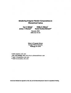
The Two-Phase Degree Reduction (TPDR) method consists of two parts. The first part schedules communications of processors that with degree greater than two. In a bipartite graph representation, the TPDR reduces the degree of maximum degree nodes by one in each reduction iteration. The second part schedules all messages of processors that with degree-2 and degree-1 using an adjustable coloring mechanism. The degree reduction is performed as follows. Step1: Sort the vertices that with maximum degree d by total size of messages in decreasing order. Assume there are k nodes with degree d. The sorted vertices would be . Step2: Schedule the minimum message mj = min{m1, m2, …, md} into step d for vertices Vi1, Vi2, …, Vik, where 1 ≤ j ≤ d. Step3: Maximum degree d = d-1. Repeat Steps 1 and 2. We first use an example to demonstrate the degree reduction technique without considering the coloring scheme. Figure 2(a) shows the communication patterns initially. The source GEN_BLOCK distribution is of (7, 10, 4, 18, 7, 18, 36). The destination GEN_BLOCK distribution is of (10, 14, 18, 14, 14, 12, 18). The redistribution is carried out over seven processors with maximum degree 3. Therefore, the communications can be scheduled in three steps. According to the above description in step 1, there are two nodes with degree 3, SP6 and DP1. The total message size of SP6 (36) is greater than DP1 (14). Thus, SP6 is the first candidate to select a minimum message (m11) of it into step 3. A similar selection is then performed on DP1. Since m5 is the minimum message of DP1 at present, therefore, m5 is scheduled into step 3 as well. As messages m11 and m5 are removed from the bipartite graph, adjacent nodes of edges m11 and m5, i.e., SP6, DP4, DP1 and SP3 should update their total message size. After the degree reduction iteration, the maximum degree of the bipartite graph will become 2. Figures 2(b) to 2(d) show this scenario. Figures 2(e) and 2(f) show the similar process of above on degree = 2 bipartite graph. In Figure 2(e), vertices SP6, SP5, SP4, SP1, DP3, DP2, DP1 and DP0 have the maximum degree 2 and are candidates to schedule their messages into step 2. According to
7 SP0
10 SP1
4 SP2
18 SP3
7 SP4
18 SP5
36 SP6
m1 m2 m3 m4 m5 m6 m7 m8 m9 m10 7 3 7 4 3 15 3 4 10 8 m11 m12 m13 6
DP1
DP0 10
DP2
14
18
DP3 14
12
7 SP0
10 SP1
4 SP2
m1 m2 m3 m4 7
3
15 SP3
10 SP1
4 SP2
15
3
7
4
3
12
DP0
DP1
DP2
DP3
DP4
DP5
14
12
18
10
11
18
14
8
12
18
18 SP5
30 SP6
7 SP4
3
4 10
DP1
DP2
DP3
DP4
10
14
18
14
14
18 SP5
8
36 SP6
m11 m12 m13 12
10 SP1
4 SP2
15 SP3
m1 m2 m3 m4 7
3
7
3
7
4 3
7 SP4
18-3
SP3
15
18 SP5
3
4
10 8
m6 m7 m8 m9 m10 m12 3 4 10 8
4
10
DP1 (2)14-3
m13
15
12
18
DP6
DP0
DP1
DP2
DP3
DP4
DP5
18
10
11
18
14
8
12
18
(2)18-8
(1)30-12
SP5
SP6
(1)36-6
SP6
m11 m12 m13
6
DP0
DP6
DP6
(e)
m1 m2 m3 m4 m5 m6 m7 m8 m9 m10 7
7 SP4
18
DP5 12
7 SP0
(b) 4 SP2
18
DP6
DP0
10 SP1
m12 m13
8
DP5
6
7 SP0
4 10
18
(d)
18 SP3
15
3
30 SP6
DP4
m1 m2 m3 m4 m5 m6 m7 m8 m9 m10 7
18 SP5
m6 m7 m8 m9 m10
7 4
(a) 7 SP0
7 SP4
12
7 SP0
(6)10 SP1
4 SP2
m1 m2 m3 m4 7
3
7
4
15 SP3
7-3
SP4
m6 m7 m8 m9 m10
15
3
4
10
8
18
DP2
DP3
DP4
DP5
DP6
DP0
18
14
14-6
12
18
(7)10
(c)
m12 m13
12
DP1 (5)11
DP2
DP3
DP4
DP5
(3)18-3
(4)14
8-8
12-12
18
DP6 18
(f)
Figure 2: The process of degree reduction (a) A bipartition graph showing communications between source processors and destination processors. (b) SP6 and DP1 have the maximum degree 3, they are marked blue. (c) m11 and m5 are scheduled. Total message size of adjacent nodes of edges m11 and m5 (SP6, DP4, DP1 and SP3) should be updated. (d) m11 and m5 are removed from the bipartite graph. The maximum degree is 2 after degree reduction. (e) SP6, SP5, SP4, SP1, DP3, DP2, DP1 and DP0 have the maximum degree 2, they are marked blue. (f) m12, m10, m7, m2 and m4 are scheduled. Adjacent nodes of edges m12, m10, m7, m2 and m4 (SP6, DP5, SP5, DP4, DP2, SP4,…) should be updated. After remove messages m7 and m10, the degree of DP3 can’t be reduced. the degree reduction method, m12, m10 and m7 are scheduled in order. The next message to be selected is m8. However, both messages of DP3 will result node contention (one with SP4 and one with SP5) if we are going to schedule one of DP3’s messages. This means that the degree reduction method might not reduce
degree-2 edges completely when the degree is 2. To avoid the above situation, an adjustable coloring mechanism to schedule degree-2 and degree-1 communications in bipartite graph can be applied. Since the consecutive edges must be scheduled into
of CS1 with CS2 and the schedule of CS3. In Row 2, messages m6 (15) and m13 (18) dominate the communication time at steps 1 and 2, respectively. This results total communication cost = 33. If we change the order of steps 1 and 2 in CS3, it becomes m13 dominates the communication time in step 1 and m12 dominates the communication time in step 2. This will result total communication cost = 30. Therefore, the colors of two steps in CS3 are exchanged in Row 3 for less communication cost. Row 4 shows communication scheduling of the adjustable coloring phase for degree-2 and degree-1 communications. The complete scheduling for this example is shown in Figure 4.
Figure 4: The scheduling of communications for the example in Figure 2.
Figure 3: Adjustable coloring mechanism for scheduling degree-2 and degree 1 communications. The bipartite graph has three CSs. Row 1 is the schedule tables of CS1 and CS2. Row 2 is the schedule table consisted of CS1 and CS2, and a schedule table of CS3. Row 3 is the same as Row 2 but the schedule table of CS3. The messages m12 and m13 are exchanged. Row 4 is the schedule table consisted of CS1、CS2 and CS3. two steps, there is no need to care about the size of messages. That means we don’t have to schedule the large messages together on purpose. Let’s consider again the example in Figure 2(e). Figure 3 demonstrates scheduling of the coloring phase for communication steps 1 and 2. To facilitate our illustration, we denote each connected component in G’ as a Consecutive Section (CS). In Figure 3, there are three Consecutive Sections, the CS1 is consisted of four messages m1, m2, m3 and m4; the CS2 is consisted of five messages m6, m7, m8, m9 and m10; the CS3 is consisted of two messages m12 and m13. A simple coloring scheme is to use two colors on adjacency edges alternatively. For example, we first color m1, m6 and m12 red; then, color m2, m7 and m13 blue; and so on. The scheduling results for CS1 and CS2 are given as shown in Row 1. Row 2 shows the merging result
The main idea of the two-phase degree reduction technique is to reduce degree of nodes by one for those nodes that have maximum degree in each reduction iteration. The following lemma states this property. Lemma 1: Given a bipartite graph G = (V, E) denotes the communications of irregular array redistribution. Let d be the maximum degree of vertices v, for all v ∈ V, a bipartite graph G’ that with maximum degree 2 will be resulted after performing d-2 times degree-reduction iterations. Proof Sketch: We use an example of degree 3 to demonstrate the above statement. For the cases of bipartite graphs with degree larger than 3, the proof can be established in a similar way. According to the characteristic of communications in irregular array redistribution we noticed that two communication links in a bipartite graph will not intersect with each other. Figure 5 shows a typical example of bipartite graph with maximum degree node is 3. There are three contiguous nodes have maximum degree 3, SPi-1, SPi and SPi+1. SPi has out-degree 3, i.e., it has three outgoing messages, mk-1, mk and mk+1 for destination processors DPj-1, DPj and DPj+1, respectively. The worst case for SPi is to incur communication conflicts with its neighboring nodes and induces itself can not schedule any communication message at the same communication step. For this scenario, we assume that if mk-2 and mk+2 are schedule at communication step 3 (the current maximum degree is 3), this will result messages mk-1 and mk+1 can not be scheduled in the same communication step (because they have common destination processor). Even so,
the degree reduction operation will select mk of SPi into step 3. Enlarge the maximum degree = d > 2, i.e., SPi will send messages to DPj, DPj+1…, DPj+d-2 and DPj+d-1. Because no two communication links would be intersected, SPi has at most two communications go into conflicts with other processors (DPj and DPj+d-1). Therefore, the TPDR algorithm can schedule one of the remaining d-2 messages of SPi into the same communication step. Therefore, we conclude that the TPDR algorithm reduces node degree by one in each degree reduction iteration. That is, a bipartite graph G’ with maximum degree 2 will be resulted after performing d-2 times degree-reduction iterations. …
SPi-1
SPi
SPi+1
…
mk-2 mk-1 mk mk+1 mk+2
…
DPj-1
DPj
DPj+1
…
Figure 5: Contiguous nodes have the same maximum degree. The algorithm of the two-phase degree reduction method is given as follows. _____________________________________________ Algorithm two_phase_degree_reduction (P, GEN_BLOCK) 1. generating messages; 2. while ( messages != null) 3. { 4. step = d = maximal degree; 5. while ( step > 2 ) 6. { 7. find_mark_blue(d); // marking degree-d nodes blue 8. sort_marked_blue_node(); // sorting blue nodes in decreasing order by message size 9. while(marked node !=null) 10. { 11. choose_marked_node(); // selecting a marked node, assume v 12. pick_minimal_message(); // schedule the minimum message (assume eij) of v into step d 13. mark_red(); // mark adjacent vertices of edge eij as red to avoid conflict communication 14. update schedule(step, message ); 15. } 16. step--; 17. } 18. coloring_message(); // color the remaining messages with maximal degree is 2 19. merge_Schedule(); // merge schedules of consecutive sections into communication steps 1 and 2 20. update schedule(step, message); 21. } end_of_two_phase_degree_reduction
_____________________________________________
4.2 Extended TPDR Based on TPDR, we present an extended two-phase degree reduction (E-TPDR) algorithm. An edge-complement operation is added in the degree-reduction phase. As the TPDR algorithm stated, the original degree-reduction operation only schedules degree-k nodes’ messages into communication step k. This might not fully utilize the available space in step k and remains heavy communications in the previous steps (less than k). Therefore, a principle for adding extra messages into these steps is to select the maximum message that is smaller than the length of current step and with un-marked adjacent vertices. The key concept of this modification is to schedule messages into communication steps during reduction phase as many as possible. Because the additional scheduled messages are with smaller message size than the current step length, the edge-complement operation will not influence the cost of original scheduling from TPDR. Figure 6 shows the communication schedule of the example given in Figure 2 using E-TPDR. Although this example does not reflect lower total cost of E-TPDR, section 5 will demonstrate the improvement of E-TPDR method from the simulation results.
S1: m1(7), m3(7), m6(15), m9(10), m13(18) S2: m4(4), m7(3), m10(8), m12(12)
S3: m11(6), m5(3), m8(4), m2(3) Figure 6: The E-TPDR scheduling communications for the example in Figure 2.
of
The algorithm of the extended two-phase degree reduction method is given as follows. _____________________________________________ Algorithm E_TPDR (P, GEN_BLOCK) 1. generating messages; 2. while ( messages != null) 3. { 4. step = d = maximal degree; 5. while (step > 2 ) 6. { 7. find_mark_blue(d); // marking degree-d nodes blue 8. sort_marked_blue_node(); // sorting blue nodes in decreasing order by message size 9. while(marked node !=null) 10. { 11. choose_marked_node(); // selecting a marked node, assume v 12. pick_minimal_message(); // schedule the minimum message (assume eij) of v into step d 13. mark_red(); // mark adjacent vertices of edge eij as red to avoid conflict communication 14. update schedule(step, message ); 15. step_length(d); // determine the length L of current step 16. sort_small_message();
// sort all messages with unmarked adjacent vertices and message size is smaller than L pick_message(); // schedule the selected messages into current step if there is no contention mark_red(); // mark adjacent vertices of the scheduled edges as red update schedule( step, message );
17. 18. 19. 20. 21. 22. 23. 24.
}
step--; } coloring_message(); // color the remaining messages with maximal degree is 2 merge_Schedule(); // merge schedules of consecutive sections into communication steps 1 and 2 update schedule(step, message);
25. 26. } end_of_ E_TPDR
4.3 Algorithmic Complexity Analysis Definition 3: Given a bipartite graph G to represent the communications of an irregular array redistribution, G’ and |E’| are denoted as the graph and the number of edges in G’ after edges are removed in degree reduction phase by TPDR, respectively. TPDR algorithm can be divided into three stages. The first part is to schedule communication messages of processors who’s degree is greater than 2. Because the scheduling in this stage is size-oriented, the time complexity of this stage is O(dPlogP), where d is the maximum degree of processors. The second stage is to schedule remaining messages after the degree reduction phase using the coloring scheme. Since we need to color all remaining edges once, according to definition 3, the time complexity in this stage is O(|E’|). The last stage is to combine scheduled tables of consecutive sections. This can be done in O(logS) via the winner tree data structure, where S is the number of consecutive sections. For the E-TPDR algorithm, the time complexity of the first stage in worst case is O(dElogE), which is different from E-TPDR algorithm. The other stages have the same complexities as TPDR algorithm.
5. Performance Evaluation To evaluate the performance of the proposed methods, we have implemented the TPDR and E-TPDR along with the divide-and-conquer algorithm [19]. The performance simulation is discussed in two classes, even GEN_BLOCK and uneven GEN_BLOCK distributions. In even GEN_BLOCK distribution, each processor owns similar size of data. The communication cost will not be dominated by specific processor, because the size of messages between processors could be very close. Contrast to even distribution, few processors might be allocated grand volume of data in uneven distribution. Since array elements could be centralized to some specific processors, it is also possible for those processors to have the maximum degree of
communications. Therefore, the communication cost will be dominated by these processors. To accomplish an optimal scheduling, it is obvious that even distribution case is more difficult than uneven distribution. This observation was comprehended by that communication cost could be determined by one processor that with maximum degree or maximum total message size in uneven distribution; consequently, it leads high probability to achieve a schedule that has the same cost as the processor’s total message size. To determine the redistribution is on even GEN_BLOCK or uneven GEN_BLOCK, we define upper and lower bounds of data size in GEN_BLOCK distribution. Given an irregular array redistribution on A[1:N] over P processors, the average block size will be N/P. In even distribution, the range of upper and lower bounds is set to ±30%. Thus, size of data blocks could be 130% N/P ~ 70% N/P. In uneven distribution, the range of upper and lower bounds is set to ±100%. Thus, size of data blocks could be 200% N/P ~ 1. 5.1 Simulation A Simulation A is carried out to examine the performance of TPDR and E-TPDR algorithms on uneven cases. We use a random generator to generate 10,000 test data sets. Figure 7 shows the comparisons of TPDR algorithm and the divide-and-conquer (DC) algorithm. We run tests by different processor numbers from 4 to 24. In 10,000 samples, the number of cases of TPDR better than DC, DC better than TPDR and the same are counted. When the number of processors is 4, there are lots of cases both algorithms have the same result. This is because that the size of messages could be larger when number of processors is less. It’s easier to derive schedules that have minimum size of total communication steps. When the number of processors becomes numerous, the TPDR provides significant improvements generally. This phenomenon can be explained by the statistic of degree-2 nodes for 10,000 test samples as shown in Figure 8. When number of processors is large, size of data blocks in these processors are relative small. Therefore, processors have lower possibility to have high degree of communication links. In other words, the number of degree-2 nodes increases largely. Since the TPDR uses an optimal adjustable coloring mechanism for scheduling degree-2 and degree-1 communications, therefore, we expect that TPDR performs better when the number of degree-2 nodes is large. This observation also matches the simulation results in Figures 7 and 9. Figure 9 gives the comparisons of the E-TPDR algorithm and the divide-and-conquer algorithm. When the number of processors is 4, there are about 60% cases has the same result by both algorithms. Similar to the previous observations, the E-TPDR performs well when number of processors is numerous.
5.2 Simulation B
E-TPDR vs DC with uneven data distribution scheme 10000 number of samples
8000 6000 4000 2000 0
6
8
14
16
18
20
22
24
93
81
73
30
29
32
58
39
19
15
4
number of processors
Figure 9: Comparison of the E-TPDR method and the divide-and-conquer algorithm on 10,000 uneven data sets (1 MB). TPDR vs DC with even data distribution scheme 10000 8000 6000 4000 2000 4
6
8
10
12
14
16
18
20
22
24
TPDR better than DC 2672 5724 5946 7658 8107 8477 8672 8951 9157 9351 9390 DC better than TPDR
8000
68
130 149 149 139 119 160 132 116 108
83
7260 4146 2905 2193 1754 1404 1168 917 727 641 527
the same
number of processors
6000
Figure 10: Comparison of the TPDR method and the divide-and-conquer algorithm on 10,000 even GEN_BLOCK test samples (1 MB).
4000 2000
4
6
8
10
12
14
16
18
20
22
24
E-TPDR vs DC with even data distribution scheme
TPDR better than DC 3134 6724 8253 8926 9288 9481 9662 9766 9811 9843 9908 884
698
555
420
293
204
168
139
76
6355 2375 863
901
376
157
99
45
30
21
18
16
number of processors
Figure 7: Comparison of the TPDR method and the divide-and-conquer algorithm on 10,000 uneven data sets (1 MB).
10000 number of samples
DC better than TPDR 511 the same
12
6550 2538 1037 435 191
the same
0
10000
0
10
DC better than E-TPDR 291 442 363 281 214 119
TPDR vs DC with uneven data distribution scheme
number of samples
4
E-TPDR better than DC 3159 7020 8600 9284 9595 9788 9861 9888 9951 9956 9964
number of samples
Simulation B is carried out to examine the performance of TPDR and E-TPDR algorithms on even cases. We also use the random generator to produce 10,000 data sets for this test. Figures 10 and 11 show the performance comparisons of TPDR and DC, E-TPDR and DC, respectively. Overall speaking, we have similar observations as those described in Figures 7 and 9. The E-TPDR performs better than TPDR. When number of processors is large, the TPDR and E-TPDR both provide significant improvements. Compare to the results in uneven cases (simulation A), the ratio of our algorithms outperform the DC algorithm become lower. We move our focus to Figure 12 to explain this phenomenon. Figure 12 gives the statistics of different degree nodes for even distribution test data. We observed that there is no nodes with degree higher than 4. In other words, the maximum degree of nodes of these 10,000 test samples is 3. On this aspect, the DC algorithm and the TPDR methods have more cases that are the same. This is also why the TPDR and E-TPDR have better ratio from 99% to 93%.
8000 6000 4000 2000 0
Statistics of degree with uneven data distribution scheme
4
6
8
10
12
14
16
18
20
22
24
number of nodes
E-TPDR better than DC 2599 5819 6916 7599 8137 8592 8810 9040 9239 9392 9463 300000
DC better than E-TPDR
250000
the same degree1
200000
0
43
64
72
86
80
84
80
58
63
64
7401 4138 3020 2329 1777 1328 1106 880 703 545 473 number of processors
degree2 degree3
150000
degree4 degree5
100000
degree6 50000
Figure 11: Comparison of the E-TPDR method and the divide-and-conquer algorithm on 10,000 even GEN_BLOCK test samples (1 MB).
0 4
6
8
10
12
14
16
18
20
22
24
number of processors
Figure 8: Statistic of degree-2 nodes in 10,000 uneven GEN_BLOCK test samples.
From the above performance analysis and simulation results, we have the following remarks. Remark 1: The TPDR and E-TPDR algorithms perform better in uneven cases than in even cases. Remark 2: The TPDR and E-TPDR algorithms perform well when number of processors is large.
Statistics of degree with even data distribution scheme 400000
[5]
number of nodes
350000 degree1
300000
degree2
250000
degree3
200000
degree4
150000
[6]
degree5
100000
degree6
50000 0 4
6
8
10
12
14
16
18
20
22
24
[7]
number of processors
Figure 12: Statistic of degree-2 nodes in 10,000 even GEN_BLOCK test samples.
[8]
6. Conclusions In this paper, we have presented a two-phase degree-reduction (TPDR) scheduling technique to efficiently perform HPF2 irregular array redistribution on distributed memory multi-computer.. The TPDR is a simple method with low algorithmic complexity to perform GEN_BLOCK array redistribution. An extended .algorithm based on TPDR is also presented. Effectiveness of the proposed methods not only avoids node contention but also shortens the overall communication length. The simulation results show improvement of communication costs and high practicability on different processor hierarchy. In HPF, it supports array redistribution with arbitrary source and destination processor sets. The technique developed in this paper assumes that the source and the destination processor sets are the same. In the future, we will study efficient methods for array redistribution with arbitrary source and destination processor sets. Besides, the issues of scheduling irregular problems on grid system and considering network communication latency in heterogeneous environments are also interesting and will be investigated. Also, we will also study realistic applications and analyze their performance.
[9]
Reference
[15]
[1]
[2]
[3]
[4]
G. Bandera and E.L. Zapata, “Sparse Matrix Block-Cyclic Redistribution,” Proceeding of IEEE Int'l. Parallel Processing Symposium (IPPS'99), San Juan, Puerto Rico, April 1999. Frederic Desprez, Jack Dongarra and Antoine Petitet, “Scheduling Block-Cyclic Data redistribution,” IEEE Trans. on PDS, vol. 9, no. 2, pp. 192-205, Feb. 1998. C.-H Hsu, S.-W Bai, Y.-C Chung and C.-S Yang, “A Generalized Basic-Cycle Calculation Method for Efficient Array Redistribution,” IEEE TPDS, vol. 11, no. 12, pp. 1201-1216, Dec. 2000. C.-H Hsu, Dong-Lin Yang, Yeh-Ching Chung and Chyi-Ren Dow, “A Generalized Processor Mapping
[10]
[11]
[12]
[13]
[14]
[16]
[17]
[18]
Technique for Array Redistribution,” IEEE Transactions on Parallel and Distributed Systems, vol. 12, vol. 7, pp. 743-757, July 2001. Minyi Guo, “Communication Generation for Irregular Codes,” The Journal of Supercomputing, vol. 25, no. 3, pp. 199-214, 2003. Minyi Guo and I. Nakata, “A Framework for Efficient Array Redistribution on Distributed Memory Multicomputers,” The Journal of Supercomputing, vol. 20, no. 3, pp. 243-265, 2001. Minyi Guo, I. Nakata and Y. Yamashita, “Contention-Free Communication Scheduling for Array Redistribution,” Parallel Computing, vol. 26, no.8, pp. 1325-1343, 2000. Minyi Guo, I. Nakata and Y. Yamashita, “An Efficient Data Distribution Technique for Distributed Memory Parallel Computers,” JSPP'97, pp.189-196, 1997. Minyi Guo, Yi Pan and Zhen Liu, “Symbolic Communication Set Generation for Irregular Parallel Applications,” The Journal of Supercomputing, vol. 25, pp. 199-214, 2003. Edgar T. Kalns, and Lionel M. Ni, “Processor Mapping Technique Toward Efficient Data Redistribution,” IEEE Trans. on PDS, vol. 6, no. 12, December 1995. S. D. Kaushik, C. H. Huang, J. Ramanujam and P. Sadayappan, “Multiphase data redistribution: Modeling and evaluation,” Proceeding of IPPS’95, pp. 441-445, 1995. S. Lee, H. Yook, M. Koo and M. Park, “Processor reordering algorithms toward efficient GEN_BLOCK redistribution,” Proceedings of the ACM symposium on Applied computing, 2001. Y. W. Lim, Prashanth B. Bhat and Viktor and K. Prasanna, “Efficient Algorithms for Block-Cyclic Redistribution of Arrays,” Algorithmica, vol. 24, no. 3-4, pp. 298-330, 1999. Neungsoo Park, Viktor K. Prasanna and Cauligi S. Raghavendra, “Efficient Algorithms for Block-Cyclic Data redistribution Between Processor Sets,” IEEE Transactions on Parallel and Distributed Systems, vol. 10, No. 12, pp.1217-1240, Dec. 1999. Antoine P. Petitet and Jack J. Dongarra, “Algorithmic Redistribution Methods for Block-Cyclic Decompositions,” IEEE Trans. on PDS, vol. 10, no. 12, pp. 1201-1216, Dec. 1999. L. Prylli and B. Touranchean, “Fast runtime block cyclic data redistribution on multiprocessors,” Journal of Parallel and Distributed Computing, vol. 45, pp. 63-72, Aug. 1997. S. Ramaswamy, B. Simons, and P. Banerjee, “Optimization for Efficient Data redistribution on Distributed Memory Multicomputers,” Journal of Parallel and Distributed Computing, vol. 38, pp. 217-228, 1996. Akiyoshi Wakatani and Michael Wolfe,
“Optimization of Data redistribution for Distributed Memory Multicomputers,” short communication, Parallel Computing, vol. 21, no. 9, pp. 1485-1490, September 1995. [19] Hui Wang, Minyi Guo and Daming Wei, "Divide-and-conquer Algorithm for Irregular Redistributions in Parallelizing Compilers”, The Journal of Supercomputing, vol. 29, no. 2, 2004. [20] Hui Wang, Minyi Guo and Wenxi Chen, “An Efficient Algorithm for Irregular Redistribution in Parallelizing Compilers,” Proceedings of 2003 International Symposium on Parallel and Distributed Processing with Applications, LNCS 2745, 2003. [21] H.-G. Yook and Myung-Soon Park, “Scheduling GEN_BLOCK Array Redistribution,” Proceedings of the IASTED International Conference Parallel and Distributed Computing and Systems, November, 1999.