while, the within-die process variation creates large discrepancy of maximum operating ... the temperature variation at the same time. On the other hand, thermal ...
2012 IEEE 6th International Symposium on Embedded Multicore SoCs
Scheduling for Multi-core Processor under Process and Temperature Variation Zheng Zhou, Junjun Gu, Gang Qu Department of Electrical & Computer Engineering University of Maryland, College Park, USA Email: (zhengzho, alicegu, gangqu)@umd.edu
reach the throughput potential when each core operates at its individual maximal clock frequency. Thermal issue is another limiting factor for each core to run at its maximal speed. When hundreds or thousands of cores are put into a single die, they make the chip power density increasingly high. High on-chip temperature not only brings up the cost of packaging and cooling, it also affects severely reliability of the circuit and may cause permanent damage. Dynamic thermal management (DTM) techniques designed for single-core processors do not work well for multi-core processors due to the spatial temperature variations and the thermal impact from core to core. Applications that have high parallelism can benefit the most from multi-core processors. Especially for computation bounded applications, massive small tasks (threads) are generated by the program with small data set and no data dependency among them, thus the memory bandwidth is not a issue. The threads carrying each task need to be assigned to cores for execution. The whole program is consider completed when the last thread/task is finished. We focus on such applications and more details will be given in Section III-D.
Abstract—Chip temperature has become an important constraint for achieving high performance on multi-core processors with the popularity of dynamic thermal management techniques such as throttling that slow down the CPU speed. Meanwhile, the within-die process variation creates large discrepancy of maximum operating frequency and leakage power among different cores across the chip. In this paper, we incorporate both temperature and process variations into the scheduling problem on multi-core processor for throughput maximization. In particular, we study how to complete a large number of threads with the shortest time, without violating a given maximum temperature constraint, on the multi-core processor where each core may have different frequency and leakage. We develop speed selection and thread assignment schedulers based on the notion of core’s steady state temperature. Simulation results show that our approach is promising to exploit the process and temperature variation for potential performance improvement on multi-core processor. For a 16-core system, when the fully parallelized program’s switching activity is less than 0.4 or the problem execution time is less than 6 seconds, we are able to achieve 31% speed-up over the system that uses the slowest core’s speed as the frequency; when the switching activity is larger than 0.5 and half of the program can be parallelized our scheduler can reduce the total processing time by 4.3%. Keywords-multi-core processor; process variation; thermal management;
A. Related Work The impact of process variation on system throughput was first studied on throughput maximization of single-core processors [2], [3], then the study was extended to multicore processors [1], [4]. The impact of process variation on the throughput of several different multi-core processors was analyzed and the sensitivities were compared in [4]. Lee et al. proposed a C2C variation model in multi-core processor and studied how to choose the active cores when number of threads is smaller than that of cores for throughput maximization [1]. However, none of the works considers the temperature variation at the same time. On the other hand, thermal issue has also been widely studied on both single core and multi-core processors. The relationship between chip temperature and leakage power on single-core processor was studied in [5]. Yeo et al. presented an analytical future temperature prediction model for multicore processors, and developed a migration policy based on the prediction model [6]. [7] formulated the multi-core temperature-aware scheduling problem as an integer linear programming problem to minimize the hot spots and temper-
I. I NTRODUCTION Technology scaling enables more and more processing cores accommodated within a single die area. Currently, CUDA architecture Fermi with 512 cores, has been put into market. The trend towards multi-core processors is motivated by the performance gain compared to single-core processors when a budget on power or temperature or both is given. The performance is expected to further increase with the increasing number of cores if thread-level parallelism (TLP) can be fully exploited. Process variation becomes a big design challenge as technology scales. Manufactured dies exhibit a large difference in maximum operating frequency (𝑓𝑚𝑎𝑥 ) and leakage power both die-to-die (D2D) and within die (WID). It is also expected that WID process variations will manifest themselves as core-to-core (C2C) 𝑓𝑚𝑎𝑥 and leakage power variations when cores within a single die becomes small enough [1]. When multi-core processors are globally clocked, 𝑓𝑚𝑎𝑥 is limited by the slowest core in the die and therefore fails to 978-0-7695-4800-5/12 $26.00 © 2012 IEEE DOI 10.1109/MCSoC.2012.9
113
ature gradients of MPSoC, and proposed an online heuristic to schedule real time tasks based on the core’s current temperature and temperature history. Rao et al. investigated both steady state temperature and transient temperature’s impact on the throughput of multi-core processors [8]. Hanumaiah et al. proposed an optimal voltage and frequency control method for maximizing the throughput of multicore processors [9]. The throttling and thread migration techniques are incorporated in [10]. Similarly, none of the works mentioned above takes the process variation into consideration together with temperature variation.
Table I C OMPARISON OF THE THREE DIFFERENT STRATEGIES .
I II III
Core 1 speed & workload 1.0 & 100 1.0 & 94 1.0 & 97
Core 2 speed & workload 1.0 & 100 0.92 & 106 1.06 & 103
Completion time 100 115 97
Throughput speed up 1.00 0.87 1.03
the core speed based on temperature and assign workload accordingly. For this example, core 1 runs at its full speed, but core 2 will gradually reduce its speed. As a result, all the workload will be complete in 97 units of time with 97 and 103 threads assigned to core 1 and core 2, respectively. 200 = 1.03. The throughput is improved to 2×97 Table 1 below summarizes the average speed and workload assignment to each core, the completion time and throughput of the system according to the three different strategies.
B. Main Contributions We consider the impact of both temperature and process variations on the scheduling problem on multi-core processors. We formulate the problem and derive analytical solutions on how to select each core’s speed to minimize the application’s completion time. We propose an efficient dynamic scheduling strategy that can achieve 1.31 speedup against the current globally synchronized system, which is the throughput upper bound.
III. P RELIMINARY A. Performance Analysis A general program consists of serial part 𝐹 and parallel part 1 − 𝐹 , which are executed separately by a single core and multi-core processor respectively. So the program’s execution time can be expressed by
II. M OTIVATION E XAMPLE We demonstrate how a multi-core processor performance, measured by throughput per core, can be affected by different strategies that control each core operating frequency and task assignment. We consider the simplest case of a 2core processor model, where core 1 maximal speed is 1.0 and the faster core 2 is 1.12; and the leakage of core 1 and core 2 are 1.0 and 1.1, respectively. We assume that the highest temperature that the cores can operate is 110𝑜 𝐶. We now compute the throughput of this processor while executing 200 units of workload, e.g. 200 identical threads each requires one unit of CPU time at the nominal speed 1.0. First, strategy I runs both cores at the nominal speed 1.0 and assigns 100 threads on each core. Both core will complete their assignment after 100 units of time and the throughput is 1 thread per core per unit of time. Clearly we see that core 2 has the potential to run faster and produce more. This leads us to strategy II which runs both cores at their respective maximal speed. 94 threads are assigned to core 1 and 106 to core 2 based on the ratio of their speeds. Core 1 will finish its assignment in 94 units of time. However, core 2 reaches 110𝑜 𝐶 after it completes 83 threads due to its higher dynamic and leakage power. The traditional ”heat and run” method will then reduce core 2 speed by half to 0.56 and complete the remaining 23 threads. As a system, 83 23 + 0.56 = 115 units the 200 threads will be completed in 1.12 200 of time, resulting a throughput of 2×115 = 0.87. Strategy II fails to improve throughput because it aggressively and statically assigns more workload to the faster core. In strategy III, we propose to dynamically adjust
𝑡𝑖𝑚𝑒 =
1−𝐹 𝐹 + 𝑆𝑠𝑒𝑟𝑖𝑎𝑙 𝑆𝑝𝑎𝑟𝑎𝑙𝑙𝑒𝑙
where 𝑆𝑠𝑒𝑟𝑖𝑎𝑙 is the speed at which serial part of program is being executed and 𝑆𝑝𝑎𝑟𝑎𝑙𝑙𝑒𝑙 is the speed at which parallel part of program is executed. With the single core speed (hence 𝑆𝑠𝑒𝑟𝑖𝑎𝑙 ) increase has already stopped due to power/thermal limit, the above formula suggests that the speedup relies on the decrease of 𝐹 or the increase of 𝑆𝑝𝑎𝑟𝑎𝑙𝑙𝑒𝑙 [11], [12]. In order to decrease 𝐹 , the program needs to be rewritten by new parallel programming model to expose more parallelism inside the program. Meanwhile more and more simple cores are put on one die to increase 𝑆𝑝𝑎𝑟𝑎𝑙𝑙𝑒𝑙 . Our paper focuses on how to improve 𝑆𝑝𝑎𝑟𝑎𝑙𝑙𝑒𝑙 with a fixed 𝐹 , a problem that is equivalent to how to minimize the completion time of a fixed number of threads. The key idea is to leverage the process variation as described next. B. Processor Model Fig 1 depicts the process variation on a 16-core processor, where each core’s maximum frequency 𝑓𝑚𝑎𝑥 (normalized to the 𝑓𝑚𝑎𝑥 of the slowest core) and leakage power 𝑃𝑠 (normalized to the 𝑃𝑠 of the least leaky core) are given [1]. We can see that both 𝑓𝑚𝑎𝑥 and 𝑃𝑠 have large variation from core to core. The fastest core is 0.65𝑋 faster than the slowest core and the most leaky core is 2.3𝑋 leakier than the least leaky one. Normally the WID process variation makes faster core also leakier.
114
D. Problem Formulation We first give a very restricted definition of the problem. After we solve the problem in the next section, we discuss how each of the constraints in the following problem formulation can be relaxed while our solution still remain valid. Given 𝑁 identical and independent threads, and a 𝑘-core processor, each core has its leakage power 𝑃𝑠,𝑖 , maximal frequency 𝑓𝑚𝑎𝑥,𝑖 and can change its operate frequency between 0 and 𝑓𝑚𝑎𝑥,𝑖 ; determine the frequency for each core to minimize the completion time of the 𝑁 threads while keeping the temperature of each core under a given threshold 𝑇𝑚𝑎𝑥 all the time. Let 𝑓𝑖 (𝑡) be the clock frequency of core 𝑖 at time 𝑡 normalized to its maximum frequency 𝑓𝑚𝑎𝑥,𝑖 , 𝑡𝑓 be the completion time of all the 𝑁 threads. As describe in the thermal model, we partition each core into 𝑚 blocks and let 𝑇𝑖 (𝑡) to be the temperature of block 𝑖 at time 𝑡, then the problem becomes to decide 𝑓𝑖 (𝑡) such that 𝑡𝑓 will be minimized under the following constraints:
Figure 1. A WID 𝑉𝑡ℎ Variation map for a 16-core processor in (a). The corresponding 𝑓𝑚𝑎𝑥 and 𝑃𝑠 map in (b) [1].
We consider a processor with 𝑘 cores, each core is independently clocked and can adjust its own operating frequency to 𝑓𝑗 𝑓𝑚𝑎𝑥,𝑗 , where 𝑓𝑗 is the scaling factor in the range of [0, 1]. We use clock gating technique to control frequency rather than voltage scaling, because clock gating induces less activation overhead and has larger margin of adjustability. We assume that each thread will be assigned to one core and each core will run a single thread at a time.
𝑘 ∫ ∑
C. Power and Thermal Model The circuit equivalent thermal model in Hotspot [13] is adopted in our work. Assuming each of 𝑘 cores has 𝑚 function units, there are 𝑘𝑚 blocks on the die and thermal interface material layer (TIM). Along with extra 14 blocks in the package, the total block number is 𝑀 = 𝑘𝑚 + 14. The multi-core processor thermal model can be expressed as the following differential equation: 𝑑𝑇⃗ (𝑡) = 𝐴𝑇⃗ (𝑡) + 𝐵 𝑃⃗ , 𝑑𝑡
𝑡𝑓
𝑓𝑚𝑎𝑥,𝑖 𝑓𝑖 (𝑡)𝑑𝑡 = 𝑁
(3)
𝑇𝑖 (𝑡) ≤ 𝑇𝑚𝑎𝑥 ∀𝑖 ∈ {1, 2, ⋅ ⋅ ⋅ , 𝑘𝑚}, 0 ≤ 𝑡 ≤ 𝑡𝑓
(4)
1
0
(5) This an optimal control problem that can be solved by dynamic programming [15], note that we will also need to include equation (3) to obtain the thermal information. However, due to the large state space (𝑁 ) and control space (𝑘), the computation is not affordable even for off-line scheduling. For the rest of the paper, we focus on finding analytical solutions that can be computed efficiently.
(1)
where 𝑃⃗ and 𝑇⃗ are 𝑀 × 1 vectors denoting power and temperature of the blocks, 𝐴 and 𝐵 are 𝑀 × 𝑀 matrices determined by thermal parameters of a given processor layout. The power on each block consists of dynamic power, which has a linear dependency on operating frequency (recall that we don’t use voltage scaling), and leakage power. We use a piecewise linear approximation model [14] to represent leakage of block 𝑖: 𝑃𝑠,𝑖 = 𝑃𝑠0,𝑖 + 𝑘𝑖,𝑠 𝑇𝑖 , where 𝑃𝑠0,𝑖 is the static power for block 𝑖 under ambient temperature and 𝑘𝑖,𝑠 is the slope the static power changes with temperature at time step 𝑠. So equation (1) can be rewritten as: 𝑑𝑇⃗ (𝑡) = 𝐴¯𝑇⃗ (𝑡) + 𝐵(𝑃⃗𝑑 (𝑓⃗(𝑡)) + 𝑃⃗𝑠0 ) (2) 𝑑𝑡 where 𝐴¯ = 𝐴 + 𝐵𝐾, 𝑃⃗𝑑 (𝑓⃗(𝑡)) represents each core’s dynamic power at its operating frequency. The package blocks does not generate power, so the package elements in vector 𝑃𝑑 , 𝑃𝑠0 are all zero. More details and discussion about this can be found in the next section.
IV. A NALYTICAL S OLUTIONS A. Steady State Throughput When 𝑁 >> 𝑘, say when the completion time 𝑡𝑓 is much longer than the time 𝑡0 needed for each core to reach its steady state temperature [8], the cores will execute at their steady state temperatures for most of the time. Then the completion time of the program will be mainly determined by the steady state throughput of each core. The problem from Section III-D then becomes to find the speed vector 𝐹⃗𝑠𝑠 at the steady state that maximize the steady state throughput. More specifically, max 𝐹𝑠𝑠
𝑘 ∑
𝑓𝑖 𝑓𝑚𝑎𝑥,𝑖
𝑑𝑇⃗𝑠𝑠 =0 𝐴𝑇⃗𝑠𝑠 + 𝐵(𝑃⃗𝑑 (𝑓⃗𝑠𝑠 ) + 𝑃⃗𝑠0 ) = 𝑑𝑡 𝑇𝑠𝑠,𝑖 ≤ 𝑇𝑚𝑎𝑥 ∀𝑖 ∈ {1, 2, ⋅ ⋅ ⋅ , 𝑘𝑚} 0 ≤ 𝑓𝑖 ≤ 1
115
(6)
1
(7) (8) (9)
perature satisfies the following differential equations: 𝑇𝑖 (𝑡) − 𝑇𝑝 (𝑡) 𝑇𝑖 (𝑡) = − + 𝑓𝑖 𝑃𝑑𝑚𝑎𝑥,𝑖 𝐶𝑖 𝑑𝑡 𝑅𝑖 +[𝑃𝑠0,𝑖 − 𝑘𝑖 (𝑇𝑚𝑎𝑥 − 𝑇𝑖 )] (10) 𝑀 𝑇𝑝 (𝑡) 1 ∑ 𝑇𝑝 (𝑡) = − + 𝑃𝑖 (𝑡) (11) 𝑑𝑡 𝑅𝑝 𝐶𝑝 𝐶𝑝 𝑖=1 Note that the time constant for the package and chip die block is of different order. For example, in the Alpha 21264, the largest time constant for chip block is 10 ms while the time constant of package is 60s [8]. Hence during 𝑡𝑠 , 𝑇𝑝 can be considered as a constant. This allows us to solve the above first order linear differential equation and obtain 𝑇𝑖 (𝑡) = 𝑇𝑖 (0)𝑒−𝛽𝑖 𝑡 + (𝛼𝑖 /𝛽𝑖 )(1 − 𝑒−𝛽𝑖 𝑡 ) Figure 2.
where 𝛼𝑖 = (1/𝐶𝑖 )(𝑃𝑠0,𝑖 −𝑘𝑖 𝑇𝑚𝑎𝑥 +𝑓𝑖 𝑃𝑑𝑚𝑎𝑥,𝑖 +𝑇𝑝 /𝑅𝑖 ) and 𝛽 = (1/𝐶𝑖 )(1/𝑅𝑖 −𝑘𝑖 ). We assume that the chip is properly designed with 𝑘𝑖 < 1/𝑅𝑖 to avoid thermal runaway. We now partition the execution interval [0, 𝑡𝑓 ] into small subintervals of length 𝑡𝑠 . 𝑡𝑠 is chosen to be of the order of 10𝑅𝑖 𝐶𝑖 so the block temperature will be in its steady state [8], [9], [13]. The steady state temperature is given by
High-level thermal model of a multi-core processor [14].
where 𝑇𝑠𝑠,𝑖 is the steady state temperature for core 𝑖 and equation (8) indicates that temperature has reach steady state and will not change with time 𝑡. This is a linear system with 𝑘 variables 𝑓𝑖 , 𝑘𝑚 linear constraints in (9), and 2𝑘 simple bound constraints in (10). It can be solved in reasonable time. Theorem 1. (Static scheduler) Suppose that at time 𝑡0 , all the cores have reached their respective steady state and have completed 𝑛𝑖 threads, then the ∑ minimum time to complete 𝑁− 𝑘 𝑛 all the 𝑁 threads is 𝑡0 + ∑𝑘 𝑓 𝑓 1 𝑖 , where 𝑓𝑖 is the solution 1 𝑖 𝑚𝑎𝑥,𝑖 to the above linear system. [Proof] We construct the scheduler that achieves this minimum completion time. On the arrival of the 𝑁 threads, we keep on feeding each core thread until time 𝑡0 . By that time, the last core has reached its steady state temperature and core ∑𝑘 𝑖 has completed 𝑛𝑖 threads. For the rest (𝑁 − 1 𝑛𝑖 ) threads, ∑𝑘 𝑓 𝑓 to core 𝑖 and set its speed we assign (𝑁 − 1 𝑛𝑖 ) ∑𝑘𝑖 𝑓𝑚𝑎𝑥,𝑖 1 𝑖 𝑓𝑚𝑎𝑥,𝑖 to be 𝑓𝑖 𝑓𝑚𝑎𝑥,𝑖 . Therefore, all∑the cores will complete their 𝑁− 𝑘 𝑛 assigned threads by time ∑𝑘 𝑓 𝑓 1 𝑖 . From the fact that 𝑓𝑖 is 1 𝑖 𝑚𝑎𝑥,𝑖 the solution to the above linear system, we know that there is no other scheduler that can finish more threads by this time. Therefore, this static scheduling strategy completes 𝑁∑>> 𝑘 𝑁− 𝑘 𝑛 threads with the minimum complete time 𝑡0 + ∑𝑘 𝑓 𝑓 1 𝑖 . 1
(12)
′
′
𝑇𝑖 = 𝛼𝑖 /𝛽𝑖 = 𝜁𝑖 𝑇𝑝 + (𝑃𝑠,𝑖 + 𝑓𝑖 𝑃𝑑,𝑖 )𝑅𝑖
(13)
′
where 𝜁𝑖 = 1/(1 − 𝑘𝑖 𝑅𝑖 ), 𝑃𝑠,𝑖 = 𝜁𝑖 (𝑃𝑠0,𝑖 − 𝑘𝑖 𝑇𝑚𝑎𝑥 ) and ′ 𝑃𝑑,𝑖 = 𝜁𝑖 𝑃𝑑𝑚𝑎𝑥,𝑖 . We assume 𝑇𝑝 can be obtained from the thermal sensor on the package, then the 𝑇𝑖 is a linear function of 𝑓𝑖 . The local optimal block frequency 𝑓𝑖 can be calculated by 𝑓𝑖 𝑓𝑖
′
′
=
[(𝑇𝑚𝑎𝑥 − 𝜁𝑖 𝑇𝑝 )/𝑅𝑖 − 𝑃𝑠,𝑖 ]/𝑃𝑑,𝑖
=
1, 𝑖𝑓 (𝑓𝑖 > 1)
(14)
Note that the core 𝑗 optimal frequency over the timestep 𝑡𝑠 is subjected to the frequency of the hottest block belonging to the core and calculated by 𝑓𝑗 = 𝑚𝑖𝑛(𝑓𝑖 )
(15)
So if we can identify those hottest blocks, the speed computation will have a considerable reduce. The equations can be reduced from 𝑚𝑘 to 𝑚. This job can be easily done by analyzing the coefficients in Eqation 13. Theorem 2. (Dynamic scheduler) With single sensor reading 𝑇𝑝 , the Eq. (14) and (15) give the local optimal core frequency in timestep 𝑡𝑠 . [Proof] In each timestep 𝑡𝑠 of dynamic scheduler, the core frequency is either maximum frequency 𝑓𝑚𝑎𝑥 or the maximum frequency at which the core can leverage all thermal headroom to maintain its temperature at 𝑇𝑚𝑎𝑥 . Any increase of the frequency results in a thermal violation. Note that the Eq. (14) and (15) involve only simple calculations, so they can be done very fast. For example, the local optimal core frequency selection of 16-core system for one time step and the frequency legalization in next section together use less than 1𝑚𝑠 on single core Pentinum 4.
𝑖 𝑚𝑎𝑥,𝑖
B. Local Optimal Frequency When the completion time is not sufficiently larger than 𝑡0 , the steady state approach cannot be used and it becomes hard to find the optimal solution. We adopt the following thermal model (shown in Figure 2) [14] and use an approximation technique to find a local optimal solution. From this equivalent thermal RC circuit, block 𝑖’s tem-
116
Figure 3.
all the system has reached the steady state or not. The timer tracks the execution time of the current parallel processing and once it reaches a pre-set value, the serial core knows that the steady state is reached. The pre-set value can be chosen as the time for the slowest core to reach its steady state temperature. Stopping the serial core from finding local optimal solution will also save its energy consumption. The run time overhead of this scheduler is hidden by two ways: first , we use the serial core to control the scheduler; second, we select the thread queue length such that it can hold threads for the fastest parallel core to complete in 2𝑡𝑠 . Therefore, while the serial core is computing, the parallel cores will not slow down or halt. Discussion on the problem our scheduling framework targets: Each thread requires same amount of computation. This assumption can be relaxed. Indeed, in some of the experiment setting, we assume that thread’s computation requirement has mean 𝑔 and the variation across threads is uniformly distributed in (0,𝑣) [15]. When we allow a thread to be executed on different cores, our results all hold. If one thread can only be run by one core, the completion time in Theorem 1 becomes a lower bound and may not be achievable. Independence of the threads. When the threads have data dependency, Theorem 1 provides a lower bound. The proposed dynamic scheduling framework can be easily modified so a thread will not be scheduled before the completion of threads it depends on. Computation bounded application. This enables us to ignore the memory problem, which is a major concern in multi-core system. Our solution can be extended to memory bounded applications by adding the notion of ready time that indicates the memory required for a thread to start is ready. However, the optimality of our result will be lost. Dynamic voltage scaling. We use clock gating to reduce frequency. Dynamic voltage scaling can be used in our framework, but it has time and energy overhead for circuit to become stable at the new voltage.
Dynamic Scheduling framework
V. S CHEDULING F RAMEWORK Based on the solutions from previous section, we develop a scheduling framework combining the static scheduler and dynamic scheduler to select speed for each core and assign threads to them. The basic idea is to let the system user input the estimated completion time 𝑡∗𝑓 of the program, if 𝑡∗𝑓 ≥ 10𝑡0 , each core will execute at its optimal steady state speed, and the thread assignment is based on the ratio of their speeds, and else if 𝑡∗𝑓 < 10𝑡0 , feeding each core the right number of threads such that it can run at its local optimal speed over the period 𝑡𝑠 . The static scheduling is very straightforward, so we mainly introduce our dynamic scheduler in the following. The local optimal solution allows the individual core frequency change to arbitrary value in [0, 𝑓𝑚 𝑎𝑥], which is impractical in real multicore processor. So a frequency legalization approach in [16] is applied to legalize each core frequency 𝑓 into 𝑟 discrete levels. Basically, we choose highest lower bounding frequency in 𝑟 to replace the 𝑓 in 𝑡𝑠 for each core. The frequency legalization also needs to be applied on optimal steady state speed. Fig 3 depicts the idea of the proposed dynamic scheduler. At the start of each parallel processing of the program, the scheduler will fill up the thread queue for each core and each core will run at its 𝑓𝑚𝑎𝑥,𝑖 . At the end of each period 𝑡𝑠 , the serial core, which is supposed to be idle during the parallel processing phase, will read the current package temperature from thermal sensor and the queue length of each parallel core’s thread queue. Using the results from the previous section, the serial core will compute the local optimal solution and do frequency legalization, and then instruct each parallel core their respective speed during the next period of 𝑡𝑠 and fill up the thread queue accordingly. This procedure repeats until all the parallel cores reach their steady state temperature. At that time, the serial core will stop solving equations (14) and (15), it simply assigns threads to parallel cores without changing their speeds. We use a timer to help the serial core to decide whether
VI. E XPERIMENT R ESULTS A. Experiment Setup In this section, we describe how we simulate the power/thermal behavior of the multi-core processor executing parallel threads. First, our dynamic scheduler reads the package temperature 𝑇𝑝 from the thermal sensor on the multi-core processor at the beginning of a period of length 𝑡𝑠 . During simulation, we use Hotspot4 [13] with LDT pairwise liberalization model (PWL) [14] to estimate the transient package temperature 𝑇𝑝 . The 𝑇𝑝 information is passed to the scheduler and the serial core will use it to compute the local optimal speed for each parallel core for that period; then Hotspot uses this speed information to estimate the new 𝑇𝑝 at the beginning of the next period.
117
Table II O PTIMAL S TEADY S TATE T HROUGHPUT OF 16- CORE PROCESSOR FOR P ROBLEMS OF D IFFERENT S WITCHING ACTIVITY
1 2 3 4 5 6 7 8 9 10 11 12 13 14 15 16 throughput gain WC 1.06 1.00 1.06 1.06 1.06 1.06 1.06 1.06 1.06 1.06 1.06 1.04 1.06 1.06 1.06 1.06 16.95 5.93% NC 1.12 1.00 1.22 1.22 1.22 1.22 1.18 1.19 1.22 1.22 1.22 1.04 1.22 1.22 1.20 1.22 18.92 18.25% BC 1.12 1.00 1.3 1.65 1.56 1.56 1.18 1.19 1.52 1.37 1.26 1.04 1.53 1.26 1.20 1.31 21.05 31.56% Table III DYNAMIC S CHEDULING AVERAGE T HROUGHPUT FOR D IFFERENT P ROBLEM S IZE
Threads 1 2 3 4 5 6 7 8 9 10 11 12 13 14 15 16 throughput 1.0e6 0.9 1.00 0.77 0.51 0.54 0.54 0.85 0.84 0.66 0.73 0.8 0.97 0.66 0.8 0.84 0.77 15.59 1.0e5 1.09 1.00 1.22 1.38 1.33 1.33 1.07 1.11 1.30 1.24 1.18 1.01 1.34 1.16 1.09 1.27 19.12 5.0e3 1.12 1.00 1.3 1.65 1.56 1.56 1.18 1.19 1.52 1.37 1.26 1.04 1.53 1.26 1.20 1.31 21.05
its 𝑓𝑚𝑎𝑥,𝑖 without violating the 𝑇𝑚𝑎𝑥 constraint. For dynamic scheduler based on Theorem 2, we are more interested to know its performance on different problem sizes (thread number) under normal switch activity. So we use 𝑈𝑛 [0.7, 0.5] distribution for thread switch activity and simulated three different problem size (N=5.0e3, N=1.0e4, N=1.0e5) to represent small problem, middle-sized problem, and large problem. Table II reports the average throughput of each single core and the sum of all cores. All throughput is normalized to that of slowest core. The average throughput is 21.05, 19.12, and 15.59 in small problem, middle-sized problem and large problem respectively. We can see that as the problem size increase, the throughput produced by dynamic scheduler is decreasing. Spectacularly, for small problem, dynamic scheduler is capable of proving the upper bound throughput; for middle-sized problem, the dynamic scheduler beats the static scheduler with 1% more throughput; for large size problem, the dynamic scheduler’s throughput is even lower than the traditional k-core system. From Eqa. (14), we know that if the dynamic scheduler runs long enough (𝑡𝑓 ≥ 𝑡0 ), the package temperature 𝑇𝑝 will eventually enter the steady state and no longer change as well as the local optimal solution, which is the steady state throughput of dynamic scheduler. It is less than the optimal steady state throughput from theorem 1. So when 𝑡𝑓 ≥ 10𝑡0 the average throughput of the program mainly depends on the steady state throughput, the static scheduler should be applied, as in our scheduling framework.
We adopt a 16-core version of the Alpha 21264 floor plan in Hotspot and set the thermal threshold 𝑇𝑚𝑎𝑥 to 110𝑜 𝐶. The convection thermal resistance value 𝑅 is configured to be 0.4𝑜 𝐶/𝑊 and the maximum dynamic power of the whole chip 𝑐ℎ𝑖𝑝𝑑𝑚𝑎𝑥 is set to be 120𝑊 . The maximum leakage power 𝑐ℎ𝑖𝑝𝑠𝑡𝑎𝑡𝑖𝑐 at 𝑇𝑚𝑎𝑥 is set to be 75𝑊 . The process variation 𝑓𝑚𝑎𝑥 and 𝑃𝑠 parameters from [1] are used to formulate different thermal/power equivalent RC circuit for each core in Hotspot. The single thread mean workload 𝑔 and the variation 𝑣 are defined by the execution time of the slowest core ( 𝑔 = 10𝑚𝑠 and 𝑣 = 5𝑚𝑠 ) in the simulation. The length of the thread queue is set to be 32. We consider the scenario that different thread in same program has different switch activity in the simulation. The thread 𝑗 power dissipation on core 𝑖 is given by 𝜌𝑗 𝑃𝑑,𝑖 where 𝜌𝑗 represents thread 𝑗’s switch activity. We set 𝜌𝑗 as a random variable with three different uniform distributions 𝑈𝑤 [1.0, 0.8], 𝑈𝑛 [0.7, 0.5], and 𝑈𝑏 [0.4, 0.1] in the simulation to represent the worst case, the normal case, and the best case that a program can have. B. The throughput of Static and Dynamic Scheduling The traditional synchronized multi-core system will use the frequency of the slowest core, core 2, as its speed and the 16-core system’s throughput will be 16 normalized to the throughput of the core 2. For different switch activity distributions, we can calculate the optimal steady state speed/frequency for each core from Theorem 1 using the upper bound of 𝜌𝑗 , as presented in the Table I. The sum of all core’s steady state speed will be the throughput produced by the static scheduler, where we can see performance gain of 5.93%, 18.25%, and 31.56% in worst case, normal case and best case respectively. The throughput increases from the decrease of switch activity is due to the fact that dynamic power is proportional to switch activity where a low switch activity will allow the cores to run at a high speed, which is shown clearly in each column in Table I. A quick comparison with the core information in Fig. 1 indicates that in best case, each core is able to run at
C. Completion Time Reduction Table III reports the completion time reduction of our proposed scheduling framework over the traditional multicore system that uses the slowest core’s speed, under normal switch activity and on middle-sized problem. We consider programs where the serial part (the 𝐹 values) counts for 10% to 50% of the total execution time. A low percentage means high parallel computation capability. The number of cores varies from 16 to 8 and to 4. We can see the clear trends of (1) larger completion time reduction with lower 𝐹 value;
118
R EFERENCES
Table IV P ERFORMANCE ( COMPLETION TIME ) GAIN WITH DIFFERENT 𝐹 AND NUMBER OF CORES . 𝑡𝑠𝑒𝑟𝑖𝑎𝑙 : SERIAL EXECUTION TIME ( S ); 𝑁 : NUMBER OF THREADS ; 𝑡𝑘,𝑝𝑎𝑟𝑎𝑙𝑙𝑒𝑙 : PARALLEL EXECUTION TIME WITH TRADITIONAL K - CORE ( S ); 𝑡′𝑘,𝑝𝑎𝑟𝑎𝑙𝑙𝑒𝑙 : PARALLEL EXECUTION TIME WITH OUR SCHEDULER ( S ); 𝑑𝑒𝑙𝑡𝑎𝑝𝑎𝑟𝑎𝑙𝑙𝑒𝑙 : PARALLEL EXECUTION TIME REDUCTION (%); 𝑑𝑒𝑙𝑡𝑎𝑡𝑜𝑡𝑎𝑙 : TOTAL EXECUTION TIME REDUCTION (%).
F 𝑡𝑠𝑒𝑟𝑖𝑎𝑙 𝑁
𝑡16,𝑝𝑎𝑟𝑎𝑙𝑙𝑒𝑙 𝑡′16,𝑝𝑎𝑟𝑎𝑙𝑙𝑒𝑙 𝑑𝑒𝑙𝑡𝑎𝑝𝑎𝑟𝑎𝑙𝑙𝑒𝑙 𝑑𝑒𝑙𝑡𝑎𝑡𝑜𝑡𝑎𝑙 𝑡8,𝑝𝑎𝑟𝑎𝑙𝑙𝑒𝑙 𝑡′8,𝑝𝑎𝑟𝑎𝑙𝑙𝑒𝑙 𝑑𝑒𝑙𝑡𝑎𝑝𝑎𝑟𝑎𝑙𝑙𝑒𝑙 𝑑𝑒𝑙𝑡𝑎𝑡𝑜𝑡𝑎𝑙 𝑡4,𝑝𝑎𝑟𝑎𝑙𝑙𝑒𝑙 𝑡′4,𝑝𝑎𝑟𝑎𝑙𝑙𝑒𝑙 𝑑𝑒𝑙𝑡𝑎𝑝𝑎𝑟𝑎𝑙𝑙𝑒𝑙 𝑑𝑒𝑙𝑡𝑎𝑡𝑜𝑡𝑎𝑙
10% 33 90000 56.1 43.5 22.4% 14.1% 112.2 96.2 14.2% 10.9% 224.4 205.3 8.5% 7.4%
20% 66 80000 50.0 37.8 24.4% 10.5% 100.0 85.8 14.2% 8.5% 200 183 8.5% 6.3%
30% 99 70000 43.7 32.2 26.3% 8.05% 87.4 74.9 14.2% 6.6% 174.8 159.9 8.5% 5.4%
40% 132 60000 37.5 27.2 27.5% 6.08% 75.0 64.3 14.2% 5.1% 150 137.2 8.5% 4.5%
[1] J. Lee and N. S. Kim, “Optimizing throughput of power- and thermal-constrained multicore processors using dvfs and percore power-gating,” in Design Automation Conference, 2009. DAC ’09. 46th ACM/IEEE, 26-31 2009, pp. 47 –50. [2] K. Bowman, S. Duvall, and J. Meindl, “Impact of die-to-die and within-die parameter fluctuations on the maximum clock frequency distribution for gigascale integration,” Solid-State Circuits, IEEE Journal of, vol. 37, no. 2, pp. 183 –190, feb 2002.
50% 165 50000 31.2 22.6 28.4% 4.3% 62.4 53.5 14.2% 3.9% 124.8 114.2 8.5% 3.6%
[3] J. Tschanz, J. Kao, S. Narendra, R. Nair, D. Antoniadis, A. Chandrakasan, and V. De, “Adaptive body bias for reducing impacts of die-to-die and within-die parameter variations on microprocessor frequency and leakage,” Solid-State Circuits, IEEE Journal of, vol. 37, no. 11, pp. 1396 – 1402, nov 2002. [4] K. Bowman, A. Alameldeen, S. Srinivasan, and C. Wilkerson, “Impact of die-to-die and within-die parameter variations on the clock frequency and throughput of multi-core processors,” Very Large Scale Integration (VLSI) Systems, IEEE Transactions on, vol. 17, no. 12, pp. 1679 –1690, dec. 2009. [5] L. Yuan, S. Leventhal, and G. Qu, “Temperature-aware leakage minimization technique for real-time systems,” in Computer-Aided Design, 2006. ICCAD ’06. IEEE/ACM International Conference on, 5-9 2006, pp. 761 –764. [6] I. Yeo, C. C. Liu, and E. J. Kim, “Predictive dynamic thermal management for multicore systems,” in Design Automation Conference, 2008. DAC 2008. 45th ACM/IEEE, 8-13 2008, pp. 734 –739.
(2) larger completion time reduction with more number of cores. For the 16-core system we take from Fig. 1, even with 𝐹 = 0.5, which means that only half of the program can be paralleled, our scheduler can reduce the total processing time by 4.3%.
[7] A. Coskun, T. Rosing, K. Whisnant, and K. Gross, “Static and dynamic temperature-aware scheduling for multiprocessor socs,” Very Large Scale Integration (VLSI) Systems, IEEE Transactions on, vol. 16, no. 9, pp. 1127 –1140, sept. 2008.
VII. C ONCLUSION
[8] R. Rao and S. Vrudhula, “Efficient online computation of core speeds to maximize the throughput of thermally constrained multi-core processors,” in Computer-Aided Design, 2008. ICCAD 2008. IEEE/ACM International Conference on, 1013 2008, pp. 537 –542.
Process variation causes significant frequency and leakage variation among cores in multi-core processor, and even worse in future. If it is not considered, the full performance of the multi-core processor is not able to be utilized or in other words, the performance is wasted. On the other hand, the dynamic thermal management plays a important role in operation of parallel program on multi-core processor due to the large range of possible die temperature. Considering process variation in DTM for maximizing multi-core processor throughput under thermal constraints is a very important problem. We formulate it as the dynamic programming problem and prove it is impossible to solve in reasonable time. We presentees theoretical heuristic solutions to the problem. We develop static and dynamic scheduling strategies basing on the solutions and propose a policy to choose between two strategies to maximize the throughput. We also demonstrate the two strategies suitable for online implementation. The proposed techniques are the first to address the problem with online solution while considering both process and temperature variation on multi-core processor.
[9] V. Hanumaiah, S. Vrudhula, and K. Chatha, “Maximizing performance of thermally constrained multi-core processors by dynamic voltage and frequency control,” in ComputerAided Design - Digest of Technical Papers, 2009. ICCAD 2009. IEEE/ACM International Conference on, 2-5 2009, pp. 310 –313. [10] V. Hanumaiah, R. Rao, S. Vrudhula, and K. Chatha, “Throughput optimal task allocation under thermal constraints for multi-core processors,” in Design Automation Conference, 2009. DAC ’09. 46th ACM/IEEE, 26-31 2009, pp. 776 –781. [11] U. Vishkin, S. Dascal, E. Berkovich, and J. Nuzman, “Explicit multi-threading (xmt) bridging models for instruction parallelism (extended abstract),” in SPAA ’98: Proceedings of the tenth annual ACM symposium on Parallel algorithms and architectures. New York, NY, USA: ACM, 1998, pp. 140–151.
119
[12] “Whitepaper: Nvida’s next generation cuda computer architecture fermi,” Sep. 2009. [13] W. Liao, L. He, and K. Lepak, “Temperature and supply voltage aware performance and power modeling at microarchitecture level,” Computer-Aided Design of Integrated Circuits and Systems, IEEE Transactions on, vol. 24, no. 7, pp. 1042 – 1053, july 2005. [14] R. Rao, S. Vrudhula, and C. Chakrabarti, “Throughput of multi-core processors under thermal constraints,” in ISLPED ’07: Proceedings of the 2007 international symposium on Low power electronics and design. New York, NY, USA: ACM, 2007, pp. 201–206. [15] D.S.Naidu, “Optimal control systems,” CRC Press, 2002. [16] B. Shi, Y. Zhang, and A. Srivastava, “Dynamic thermal management for single and multicore processors under soft thermal constraints,” in Low-Power Electronics and Design (ISLPED), 2010 ACM/IEEE International Symposium on, 2010, pp. 165 –170.
120