apply particle filter sequential Monte Carlo methods to im- plement multiple sensor scheduling for target tracking. Un- der the constraint that only one sensor can ...
SCHEDULING MULTIPLE SENSORS USING PARTICLE FILTERS IN TARGET TRACKING Amit S. Chhetri, Darryl Morrell and Antonia Papandreou-Suppappola Department of Electrical Engineering, Arizona State University, Tempe, Arizona 85287, USA ABSTRACT A critical component of a multi-sensor system is sensor scheduling to optimize system performance under constraints (e.g. power, bandwidth, and computation). In this paper, we apply particle filter sequential Monte Carlo methods to implement multiple sensor scheduling for target tracking. Under the constraint that only one sensor can be used at each time step, we select a sequence of sensor uses to minimize the predicted mean-square error in the target state estimate; the predicted mean-square error is approximated using the particle filter in conjunction with an extended Kalman filter approximation. Using Monte Carlo simulations, we demonstrate the improved performance of our scheduling approach over the non-scheduling case. 1. INTRODUCTION Sensor technology has become important for commerce, environmental science, medicine, defense, etc. The last two decades have seen an unprecedented growth in the number and variety of sensors and methods to extract information from sensor measurements. Cost effective sensor use is imperative for effective system performance. Sensor scheduling, which is the allocation of sensing resources over time, is thus becoming an essential component of sensor systems. The problem of scheduling sensors to optimize the expected cost function over time is a stochastic control problem; in principle, solutions to this problem can be computed using dynamic programming [1, 2]. In practice, computing optimal solutions may be prohibitively expensive, and suboptimal greedy algorithms are used instead [3–5]. Some cost functions used in scheduling algorithms include sensor usage cost, accuracy of sensor state estimate, cost of resources, (weighted) squared error and desired estimate covariance [6]. Recently, information theoretic cost functions that measure the difference between prior and posterior distributions have been applied together with particle filter sequential Monte Carlo techniques [3, 4, 7]. In this paper, we minimize the mean squared estimate error. This work was supported by a Raytheon contract with Integrated Sensing and Processing DARPA program.
Specifically, we schedule infrared (IR) and radar sensors to obtain measurements, and track the target based on the measurements using a particle filter. The sensors are scheduled using the particle filter and an extended Kalman filter (EKF). The scheduling algorithm predicts multiple steps ahead (where each step corresponds to a time difference ) to find the sensor sequence that minimizes the estimated covariance at those steps. Monte Carlo simulations show that the tracking performance improves significantly with sensor scheduling. 2. PROBLEM FORMULATION We consider a target moving in a 2-dimensional Cartesian be a real-valued random vector denoting the space. Let target state at time � . The state vector is defined as
�
�
�
�
�
��
�
�
where � and � are the positions in the � and � directions, � and � are the velocities in the � and � directions, and � denotes matrix transpose. The target evolves according to a linear system driven by white Gaussian noise as
�
�
��
��
�
(1)
Here, � models the state kinematics: �
� � � � ��� � � � � �
� � � � � � �
� � �� �
is the time difference between measurements, and � is a Gaussian random vector with covariance �. This covariance is obtained by converting a continuous time stochastic target model into an equivalent discrete time model [8]: �
��
�� � � ��� � � ��
�
� �
��� �
� �
� �
�� � ��� �
� �
� � �
� ��� � � �
Here, � is a scalar that determines the intensity of the process noise. The dynamics model in (1) is Markov and can . be represented by the conditional density � A radar and an IR sensor are located at the origin; each sensor provides three measurements: range , range rate and azimuth angle . The IR sensor provides a good measurement of the azimuth angle while the radar sensor provides a good measurement of the range and range rate of the target. The accuracy of the measurements depends on the sensor type; we model the relative accuracy by using different observation noise covariance matrices for each sensor. The measurements are arranged as a vector � � at time �
�
where the measurement (and hence the weights) at time � depend on the sensor � . An approximation to the posterior density using the particles is
�
�
�
��
�
�
��
��
��
�
�
���� �� �� �� ���
� �
�
�
�
�
�
���
�
�
�
�
�
�
�
�
�
���
�
�
�
� �
(2)
�����
�
� � �
�
�
�
(3)
��
��
�
� � ��
�
�
�
�
�
��
�
�
�� �
(4)
4. SENSOR SCHEDULING
Tracking is the problem of inferring the motion of an object from observations. Given the conditional densities � and � �� , the state can be estimated recursively using a particle filter [9,10]. The particle filter belongs to the class of Sequential Monte Carlo filters. It is an asymptotically optimal implementation of a Bayesian filter based on samples (particles) and associated importance weights. An advantage of the particle filter is that it can be used for nonlinear systems with non-Gaussian noise. It is used in this work to handle the nonlinearity of the measurement model as well as to allow for non-Gaussian noise. We present the particle filter algorithm specific to our ����� at time work [9]. The posterior density function � � is approximated by a set of particles or random samples �� � � � � � � � � � � and associated weights �� � � � � � � � � � � �. Here, � � and � � represent the measurements and sensor selection, respectively, from time to � . At each time � , the particles are drawn from a proposal dis� tribution � � � � � , and the predicted par����� � . ticles approximate the predicted state density � The particles are assigned weights which depend on the measurement at time � using the recursive weight equation [9]
�� �
�
�
�
3. TARGET TRACKING ALGORITHM
�
��
�
Note that resampling may be used to eliminate particles with low weights [9]. In such a case, all the weights become equal to �� .
�
��
�
� Æ
and the error covariance matrix can be obtained as
and �� is Gaussian with covariance matrix � � . The conis denoted by � � � . ditional density of � � given
�
� � �
��
� �� � � ��
� ��
�
��
where �
�����
Using (2), an approximate minimum mean square error (MMSE) estimate of the state can be obtained as [9]
where � denotes the selected sensor and is either or to denote use of the IR or the radar sensor, respectively. The measurements are nonlinearly related to the state as
��
�
�
�
�
In the following, we develop a sensor scheduling algorithm for two sensors that can be extended to multiple sensors without loss of generality. In our work we use the mean squared error (the trace of the error covariance matrix � ) � �� as the cost function. In the following, we denote as � ���� �� �� the approximate predicted covariance at time � � obtained using the sensor sequence � � � �� � � � � � � � � �� . We assume that at any given time, only one of the two sensors may be used. The scheduling algorithm is initialized at time � by the predicted estimate and its covariance computed using (3) and (4); the observation function � � is linearized about this estimate, and the resulting Jacobian is used in the EKF equation to compute the predicted estimate � covariance � ���� � for each sensor. When minimizing over one sensor use, we choose � � to minimize the trace � of � ���� � . For � step sensor scheduling, the total number of possible sensor sequences is ; we minimize the total squared error by exhaustive computation over all possible sensor sequences. For each sequence, the error covariance for times � through � � is predicted using the standard EKF equations for the estimate error covariance, and the total � ��� �� �� squared error �� ��� �� � is computed. We then choose the sequence of sensor uses that gives the minimum total squared error. Once the optimal sequence of sensors is selected, measurements are obtained and the target state estimate is computed using the particle filter. The proposed multiple step scheduling process is summarized in Table 1.
�
�
�
�
��
�
�� ��
�
2700
End
2600
For each possible sequence of sensors �
� � ��� � �
� �
� � �
and �
2400
�
Define
�
For �=1 to � , � Project the estimate and covariance matrix:
Compute the Jacobian matrix
�
� �
�� �
�
1900
��
��
1800
1700 −2000
��
� �
Ü��Ü
�
�� �� �
End Calculate the total cost for � �� ��� ��
�
�
��
�
� �� �� � ��� ��
�� ��� ��
5. SIMULATIONS AND RESULTS We simulate a target trajectory in a 2-dimensional plane as shown in Figure 1. The target starts at �� � =(10000, 2000) � m. The initial velocity of the m and ends at � target in the � and � directions is -300 m/s and -50 m/s, respectively. The sensors are fixed at the origin, and the target and � are chosen to be 1 moves for 35 s. The values of s and 200, respectively. The measurement error covariance matrices for the IR and radar sensors were chosen such that the IR sensor has high accuracy in azimuth angle, while the radar has high accuracy in range and range rate. The matrices used in the simulations are as follows �
� �
� � � ��
� � � � � � ���� �� � � � � � �� � � ������ For the particle filter algorithm we chose � � ��� parti-
��� �� � � ��� � � ��� � �
5
10
15
20
25
30
35
40 NS M=1 M=2 M=3
0
5
10
15
20
25
30
35
40
cles, and a total of 300 Monte Carlo simulations were run.
NS M=1 M=2 M=3 0
5
10
15
20
25
30
35
40
40
�
Table 1. Multiple step sensor scheduling algorithm.
� ���� �����
0
40
20
y−vel
NS M=1 M=2 M=3
60
End Choose the optimal sequence of sensors as � � � �
10000
20
10
�� �� � � ������ ���� �
8000
30
� � �
�
��
6000
40
20
�
� � ��� ��� �� � �� � �� ���� �� ��
4000
60
x−vel
�
2000
Fig. 1. Simulated trajectory of the target.
�
� ��
�� ��
��
0
x (m)
Update the projected error covariance matrix �� �� ���� �� ��
�
� ��
�� ��
��
Start 2000
y−pos
�
��
� � � �� � �
�
2200
2100
x−pos
�
y (m)
2300
��� �� � � �� � �� � ������ ���� � � � � � ����� ��� ��� �
�
2500
NS M=1 M=2 M=3
20
0
0
5
10
15
20
25
30
35
time (s)
Fig. 2. Comparison of the variances for the NS case and the � � , and step scheduling cases.
�� �
�
The initial particles are generated as samples from a Gaussian distribution whose mean is the true location and whose covariance matrix is �
� � � �� � � ���� We compare the tracking results of � � �� � and � step �� � � �� � � � � �
� ���� � �
� � �� �
sensor scheduling with the case of no-scheduling (NS). For the NS case, we use only the radar sensor. A comparison of variances (in dB) of the position and velocity estimates for � and and NS cases can be seen in Figure 2. the � We can observe that for the scheduling cases, the variances decrease with time while for the NS case the variances level out after an initial drop. This is more evident for the � position (top plot in Figure 2) since the NS radar case does not provide an accurate azimuth angle measurement. Figure 3
���
�
40
65
We are also investigating the computation of the predicted cost function using the particle filter directly rather than the EKF approximation that can lead to errors for non-linear and non-Gaussian systems.
NS M=1 M=2 M=3
60
55
MSE (dB)
50
45
40
7. REFERENCES
35
30
25
0
5
10
15
20
25
30
35
40
time (s)
Fig. 3. Comparison of the MSE for the NS case and the � � , and step scheduling cases.
�� �
�
[2] D.A. Castanon, “Approximate dynamic programming for sensor management,” in Proceedings of the 36th IEEE Conference on Decision and Control, 1997, vol. 2, pp. 1202–1207.
2800 True NS M=1 M=2 M=3
2600
y (m)
2400
2200
2000
1800
1600
1400 −2000
0
2000
4000
6000
8000
10000
[1] V. Krishnamurthy, “Algorithms for optimal scheduling and management of hidden Markov model sensors,” IEEE Transactions on Signal Processing, vol. 50, pp. 1382–1397, June 2002.
12000
[3] F. Zhao, J. Shin, and J. Reich, “Information-driven dynamic sensor collaboration for tracking applications,” IEEE Signal Processing Magazine, vol. 19, no. 2, pp. 61–72, March 2002.
x (m)
Fig. 4. Comparison of the tracked target for the NS case and � , and step scheduling cases. the �
�� �
�
illustrates a comparison of the MSE for different scheduling cases. It can be seen that the MSE decreases with time for the scheduling cases while it levels out for the NS case. At time � , the difference in MSE between the NS dB in Figure 3. Figure and scheduling cases is about 4 compares the tracked trajectory for the various scheduling cases. It is seen that the tracking performance for the scheduling cases is much better than the NS case. Similar results were obtained when an IR sensor was used instead of the radar sensor for the NS case. It should also be noted that � , the tracking performance is comparable for the � and step sensor scheduling.
� ��
��
���
�
6. CONCLUSIONS We have developed a sensor scheduling algorithm for target tracking using a particle filtering approach. Specifically, we used the particle filter and EKF to project multiple steps ahead and minimize the MSE using the predicted covariance obtained from all possible sensor sequences. Monte Carlo simulations of our algorithm reveal that the tracking performance using sensor scheduling is superior to the noscheduling case. Note that the use of the MSE as a cost function does not take into account the non-diagonal elements of the error covariance matrix. Thus, we plan to further improve our scheduling performance using the difference between predicted and desired error covariance matrices as suggested in [6] for non-particle filter applications.
[4] C. Kreucher, K. Kastella, and A. Hero, “A Bayesian method for integrated multitarget tracking and sensor management,” in Proceedings of 6th International Conference on Information Fusion, 2003. [5] A. Logothetis and A. Isaksson, “On sensor scheduling via information theoretic criteria,” in Proceedings of the 1999 American Control Conference, 1999, vol. 4, pp. 2402–2406. [6] M. Kalandros and L.Y. Pao, “Covariance control for multisensor systems,” IEEE. Trans. on Aerospace and Electronic Systems, vol. 38, pp. 1138–1157, October 2002. [7] A. Doucet, B.N. Vo, C. Andrieu, and M. Davy, “Particle filtering for multi-target tracking and sensor management,” in Proceedings of the Fifth International Conference on Information Fusion, 2002, vol. 1, pp. 474–481. [8] P. Maybeck, Stochastic Models, Estimation, and Control, Academic Press, 1979. [9] M.S. Arulampalam, S. Maskell, N. Gordon, and T. Clapp, “A tutorial on particle filters for online nonlinear/non-Gaussian Bayesian tracking,” IEEE Trans. on Signal Processing, vol. 50, pp. 174–188, February 2002. [10] A. Doucet, N. de Freitas, and N. Gordon, Eds., Sequential Monte Carlo Methods in Practice, SpringerVerlag, 2001.