60
IEEE TRANSACTIONS ON ROBOTICS AND AUTOMATION, VOL. 17, NO. 1, FEBRUARY 2001
Scheduling No-Wait Production with Time Windows and Flexible Processing Times Fabrice Chauvet, Jean-Marie Proth, Member, IEEE, and Yorai Wardi, Member, IEEE
Abstract—This paper presents a low-complexity algorithm for on-line job scheduling at workcenters along a given route in a manufacturing system. At each workcenter, the job has to be processed by any one of a given set of identical machines. Each machine has a preset schedule of operations, leaving out time-windows during which the job’s processing must be scheduled. The manufacturing system has no internal buffers and the job cannot wait between two consecutive operations. There is some flexibility in the job’s processing times, which must be confined to given time intervals. The scheduling algorithm minimizes the job’s completion time, and it is executable in real time whenever the job requirement is generated. Index Terms—No-wait manufacturing, on-line scheduling, time windows.
I. INTRODUCTION
T
HIS paper considers an on-line job scheduling problem in no-wait manufacturing. The underlying manufacturing system is configured for multiple products. Whenever a product demand arrives a corresponding work order is generated, involving job processing at various workcenters. By “job” we mean a part, component, or workpiece that is processed by machines stationed at the various workcenters. Job processing by a machine is called an operation. Some operations are sequential and following a given order, while other operations must process multiple jobs in a concurrent fashion, as in the case of assembly. We characterize the work order by its associated jobs’ routes and processing times at the various workcenters. To simplify the notation (and exposition), we identify the workcenters with production stages, and assume that only one type of operation can take place at each workcenter. We comment that the meaning of the term “job” can be extended to include batches or lots of parts. Consider a particular product demand arising at time , and the associated work order, also generated at that time. The jobs’ routing is given and is dependent on the product in question. Each workcenter contains one or more identical machines, only one of which is required for processing the related jobs. A maManuscript received March 5, 1999; revised February 18, 2000. This paper was recommended for publication by Associate Editor D. Wu and Editor N. Viswanadham upon evaluation of the reviewers’ comments. The work of Y. Wardi was supported by National Science Foundation under Grant INT-9402585. This paper was presented in part at the IEEE/EAMRI Rensselaer’s International Conference on Agile, Intelligent, and Computer-Aided Manufacturing, Troy, NY, October 1998. F. Cauvet is with INRIA Lorraine, 57070 Metz, France. J.-M. Proth is with the Institute for Systems Research, University of Maryland, College Park, MD 20742 USA. Y. Wardi is with the School of Electrical and Computer Engineering, Georgia Institute of Technology, Atlanta, GA 30332 USA (e-mail:
[email protected]). Publisher Item Identifier S 1042-296X(01)02768-9.
chine can process only one job at a time. At time , each machine in the system has a preset schedule of activities like maintenance or previously scheduled processing of other jobs. The scheduling problem for the present work order, generated at time , is to schedule all of its associated jobs at the various workcenters according to their routes in order to minimize the product’s completion time without interfering with any of the machines’ preset activity schedules. This scheduling must be performed at time . Once determined, a job’s schedule cannot be modified, and it becomes part of the associated machine’s activity schedule. The product’s completion time is defined as the time its last job processing is completed. The no-wait characteristic of the system implies the absence of internal buffers, and therefore jobs must be “in processing” continually while following their routes. Times required for transportation, loading, and unloading can be assumed negligible if they are small as compared to the processing times by machines. Alternatively, these tasks may be considered as manufacturing operations that must be scheduled if they require significant times. There is flexibility in the processing times: depending on the product type, the job, and the particular workcenter, there is a given interval that must contain the job’s processing time. We summarize and clarify. A product demand arriving at time causes a work order to be generated at that time. The work order corresponds to jobs’ routing through the system. Each workcenter contains one or more identical machines for processing the various jobs. Each machine has an associated finite set of time intervals during one of which the jobs’ scheduling must take place. The processing time has to fall within a given (machine- and job-dependent) interval. Jobs are not allowed to wait once they enter the system. The scheduling problem amounts to computing, at time , the schedule that minimizes the product’s completion time. The following three scheduling parameters have to be determined: 1) jobs’ release times, namely the times jobs are put into the system; 2) the choice of a machine at each workcenter along the job’s route; 3) the processing times at the various machines. In what follows, we propose a low-complexity algorithm for real-time solution of this scheduling problem. The above scheduling problem resembles the problem of production rescheduling in dynamic manufacturing environments, where a schedule is updated as events occur. However, the problem here is not that of rescheduling, but rather that of computing a schedule for each product demand. The computation of each schedule, done in real time, depends on past
1042–296X/01$10.00 © 2001 IEEE
CHAUVET et al.: SCHEDULING NO-WAIT PRODUCTION WITH TIME WINDOWS AND FLEXIBLE PROCESSING TIMES
Fig. 1.
61
An example with assembly–disassembly operation.
schedules via the time windows resulting from them. Therefore, the optimal scheduling problem can be viewed as an optimal control problem, and hence it will be termed a scheduling control problem. Questions of manufacturing-systems control requiring on-line solutions have become quite important in recent years. Due to decreasing product life cycles, planning horizons are becoming shorter, and future tools for planning and scheduling will be expected to provide immediate (on-line) solutions. At the same time, many companies are diversifying their product lines while keeping inventory levels to a minimum. All of this highlights the importance of scheduling control in no-wait manufacturing environments. Some processes (e.g., chemical) have flexibility in processing times. Otherwise, such flexibility reflects on machines’ ability to briefly hold semi-finished products, which can compensate for the absence of buffers.1 The problem of scheduling a given set of operations on semiidentical processors (identical, according to our terminology) with availability time intervals was considered by Schmidt [8], [9]. These references concerned feasibility, and developed lowcomplexity algorithms for computing feasible schedules. The present paper is different in that it concerns optimality, and it imposes assumptions guaranteeing feasibility. Scheduling in no-wait manufacturing has been extensively discussed in the literature, often in the context of systems with blocking. Callahan [1] used queueing models to study no-wait problems in the steel industry. Chu et al. [4] and Chauvet et al. [2] have considered surface treatment problems with no-wait models. McCormick et al. [6] have studied a cyclic flowshop with buffers, which can be transformed into a blocking problem by considering the buffers as resources with arbitrary processing times. Hall and Sriskandarajah [5] presented a survey of scheduling problems with blocking and no-wait, and Rachamadugu and Stecke [7] have classified scheduling procedures in no-wait environments. The above references either constrain the processing times to be given and fixed [4], [6], [7], or allow considerable flexibility in their values [2], [5]. This paper permits some flexibility in the processing times by allowing them to assume values from within given intervals. It differs from the existing works in that it allows neither waiting nor blocking,2 and thus addresses a scheduling problem in a new context that has not been explored yet. A preliminary version has been presented [3]. 1In this case, the term “no wait” is not quite precise since there is waiting at the machines. However, that term is made precise by referring to the model which incorporates the holding time within the processing time. 2Again, when flexible processing times represent the possibility of holding a part by a machine then certainly there is blocking, but the model having flexible processing times can be viewed as excluding the possibility of blocking.
The rest of the paper is organized as follows. Section II formulates the problem and establishes the requisite notation. Section III develops the algorithm and carries out its analysis, while relegating some of the proofs to the Appendix. Section IV provides an example, and Section V concludes the paper. II. PROBLEM FORMULATION Consider a product demand and its associated work order. Suppose that the work order involves a finite set of operations, denote the cardinality of the set denoted by , and let . The operations are indexed by and denoted by . For example, see Fig. 1 involving assembly and disassembly and , and operations. In this example, the work order involves multiple (two) jobs. Each operation is associated with a workcenter, and each workcenter contains one or more identical machines. Each one of these machines can perform the operation in question. The routing of jobs, associated with the work order, among the various workcenters is given in the example of Fig. 1. , the following notation will be used: For every —the set of operations immediately preceding ; • —the set of operations immediately following ; • —the set of operations other than that must begin • ; at the same time as —the set of operations other than that must end at • . the same time as ( is an assembly For example, in Fig. 1, because must end at the same time operation), because no other operation must end at the as , and same time as . To simplify the exposition we will sometime with the index , and thus will say that identify the operation . Also, we will implicitly assume that a specific operation can be required no more than once for a given work order. We assume that no part can wait for an operation, that is, , must start at the time ends. Moreover, it for and , then can be seen that, if and . We observe that, in the case of an assembly then , and in the case operation, if then . We assume of disassembly, if ( , respectively) then there exists a the contrary: if corresponding disassembly (assembly, respectively) operation and , that is, there preceding (following, respectively) ( , respectively). This later exists assumption is not restrictive in view of the general definition of “operation,” possibly including loading/unloading and material transport.
62
IEEE TRANSACTIONS ON ROBOTICS AND AUTOMATION, VOL. 17, NO. 1, FEBRUARY 2001
Next, let and denote the beginning and ending times, denote the processing respectively, of , and let . Given and , let time of be the given interval that must contain , that is, we impose the . requirement that , there exists a finite set Suppose that, for every operation , [for of closed time intervals, denoted by ], during one of which must take some given integer place. These time intervals, henceforth called time windows, or windows, reflect periods during which the various resources are available for the operation . We observe that several windows may be overlapping since they can be associated with various must be peridentical machines at the workcenter where and the starting time and end formed. Denoting by , we have that . We order these time of , and windows in the increasing order of their starting times in case of two identical starting times, in the increasing order of . We also assume that , that is, their end times the last window’s end point, for each operation, is . This assumption implies that there exits at least one feasible schedule which can be obtained by choosing a late window, and it allows us to focus on the problem of optimality. In summary, the work order involves the operations . The operations’ precedence relations and jobs’ , , , and , associated routing are given by the sets . Moreover, for every , we are given with every and in whose terms the processing time of numbers will be constrained, and a set of time windows [for ], , , during one of a given integer must take place. which the operation Definition 2.1: A feasible schedule consists of operations , , beginning at time and ending at time , sat. isfying the following four constraints for all For some and for every for every
(2.1) (2.2) (2.3)
and for every
(2.4)
Observe that (2.1) expresses the requirement that the operation be performed during one of the time windows, (2.2) imposes upper and lower bounds on the processing time, and (2.3) and (2.4) define the routing and precedence relations among the jobs and express the fact that no waiting is allowed. The scheduling control problem is to choose a feasible schedule that minimizes the product completion time. That is, such that (2.1)–(2.4) are satisfied and to compute the last operation ends at the earliest possible time. In formal by , terms, let us define the set namely the set of indices whose corresponding operations are at the “end of a line,” and observe that the completion time is . the term An algorithm for this purpose will be developed in Section III.
III. ALGORITHMS This section presents an algorithm for computing the feasible schedule that minimizes the product completion time. Consider , and the undirected graph whose nodes are the operations and iff where there is an arc between the operations . Recall that, by assumption, ( , respectively) ( , if and only if there exists an operation respectively). Assumption 3.1: The above undirected graph is loop free. We remark that this assumption excludes the case of an assembly operation combining two jobs that originated from the same disassembly operation. In what comes we identify an index with the operation for the sake of notational convenience. Thus, for example, we instead of . will use the notation in a sequence We next renumber the operations in a way that will be useful for the scheduling control must be at the start algorithm, below. The first operation or the end of a line, namely, have no preceding or succeeding , either is at the start or the end of a operations. For line, or all of its preceding or succeeding operations must have been numbered. The sequencing is done according to Algorithm denote the set of operations that have been 3.1, below. Let is considered, namely numbered when the operation , and define . Observe that while . Algorithm 3.1: Step 0) Set . Step 1) Choose to be any operation satisfying either one of the following two conditions: 1) 2)
.
Step 2) Set . If , go to Step 1. If , exit. Note that must be at the start or the end of a , if 1) is satisfied then every operline. For has been numbered, and if 2) is ation in has been satisfied then every operation in numbered. Proposition 3.1: Algorithm 3.1 is consistent in the sense that of all of the operations. it results in a sequencing Proof: The proof is immediate in view of Assumption 3.1. We note that the sequencing resulting from Algorithm 3.1 is by no means unique. We next develop the scheduling control algorithm. Recall that is carried out during a time window for operation . some is a standard Definition 3.1: A set of windows window set if it contains one window associated with each there exists workcenter, namely, for all such that . is feasible with Definition 3.2: A schedule if it is a respect to a standard window set , the operation is feasible schedule and for every
CHAUVET et al.: SCHEDULING NO-WAIT PRODUCTION WITH TIME WINDOWS AND FLEXIBLE PROCESSING TIMES
performed during the time window namely, the following inequalities hold [see (2.1)]: and
,
(3.1)
Definition 3.3: A schedule is minimal feasible with respect if it has the least completion time to a standard window set among the schedules that are feasible with respect to . Definition 3.4: A schedule is optimal if it solves the scheduling control problem, namely, it is a feasible schedule with the earliest-possible product completion time. If we could compute a minimal feasible schedule with respect to every standard window set, then the schedule among them with the earliest completion time would be optimal. This approach for solving the scheduling control problem could be impractical for two reasons as follows: 1) not every standard window set has a feasible schedule, and 2) the number of stan—indicating an exponential comdard window sets is plexity. We get around the first difficulty by relaxing the feasibility requirement and note that the second difficulty also will be overcome, as it will be seen below. Recall that the feasibility requirements are given in terms of (2.1)–(2.4) or (3.1) in lieu of (2.1). is almost feaDefinition 3.5: A schedule if sible with respect to a standard window set all of the feasibility requirements are satisfied except possibly for the right inequality of (3.1), i.e., we permit the condition . is minimal almost Definition 3.6: A schedule if it is almost feasible with respect to a standard window set and, for every other schedule feasible with respect to that is almost feasible with respect to , the inequaland hold for every . ities [the right inequality Removing the requirement of (3.1)] ensures that every standard window set has an almost-feasible schedule. Consequently, every standard window set has a minimal almost-feasible schedule. Algorithm 3.2, below, computes such a minimal almost-feasible schedule with . One among the schedules computed by Alcomplexity gorithm 3.2, taken over the range of standard window sets, will be shown to constitute an optimal schedule. Still the complexity of standard window issue, indicated by the number sets, remains. However, we address it by devising a procedure standard window requiring a search among at most sets. The following algorithm computes a minimal almostfeasible schedule with respect to a standard window set . It has two steps: the first step computes and , respectively, lower bounds on and , denoted by and the second step uses these bounds to compute a desired schedule (the minimal almost-feasible schedule is not unique). are computed by a forward recursion The bounds is computed by a backward while the schedule recursive procedure. . As Given a standard window set and by for Algorithm 3.1, we define the sets with , and .
63
Algorithm 3.2: Step 1: Forward computation of lower bounds. For , compute and according to either Case I or Case II, below (we later will see that if the conditions defining both cases are satisfied then the resulting computations are identical):. . Case I: Set
(3.2) and set
(3.3) .
Case II: Set
(3.4) and set
(3.5) Step 2: Backward computation of the schedule. For every , compute and according to either one of the following respective cases. . Set for any , Case 1: . and set . Set for any , Case 2: . and set . Set for any , Case 3: . and set . Set for any , Case 4: . and set , and Case 5: None of the cases 1–4 is satisfied. Set . set Some of the variables in Algorithm 3.2 can be computed in more than one way. We say that such a variable is well defined if it has a unique value regardless of the way it is computed. In the forthcoming we will prove that all of the variables computed by the algorithm are indeed well defined. Proposition 3.2: All of the variables computed by Algorithm 3.2 are well defined. The proof is highly technical and is relegated to the Appendix. The next assertion concerns the minimality of the schedule computed by Algorithm 3.2.
64
IEEE TRANSACTIONS ON ROBOTICS AND AUTOMATION, VOL. 17, NO. 1, FEBRUARY 2001
Proposition 3.3: For a given standard window set , the schedule computed by Algorithm 3.2 is minimal almost feasible with respect to . The proof requires some preliminary results, whose proofs are supplied later in order not to break the flow of the argument. that is almost Lemma 3.1: For every schedule and for all feasible with respect to , . ( and were computed by Algorithm 3.2 and are independent of the schedule.) that is almost Lemma 3.2: For every schedule feasible with respect to , and for every and
(3.6)
Lemma 3.3: For every and Lemma 3.4: For every equalities hold:
(3.7) , the following in-
(3.8) Lemmas 3.1 and 3.3 will be required for proving Lemmas 3.2 and 3.4, which will be directly applied to the following proof of Proposition 3.3. Proof of Proposition 3.3: Consider first the almost feasicomputed by Algorithm 3.2 bility of the schedule (minimality will be addressed later). Equations (2.3) and (2.4) follow from the fact that the quantities computed by Algorithm 3.2 (Step 2) are well defined; see Proposition 3.2. Regarding (2.1) [alternatively, (3.1)], the left inequality follows from the , (Lemma 3.2), and the fact that right inequality is not necessary for almost feasibility. Finally, (2.2) follows from Lemma 3.4. Consequently, the schedule is almost feasible with respect to . Its minimality follows from Lemma 3.2. We next prove the above lemmas , Proof of Lemma 3.1: We argue by induction. For and . by Step 1 of Algorithm 3.2, At the same time, since is almost feasible, the left inequality and, by (2.2), of (2.1) implies that . This establishes that and . and consider the following inductive Fix , and hypothesis: “For every .” We now prove such inequalities for . and Since is almost feasible, . Moreover, for every , and ; for , and ; for every , every and ; and for every , and . Therefore, the following two inequalities apply:
(3.9) and,
(3.10) and as computed in Step 1. In Case I, Now consider is given by (3.2). By the inductive hypothesis each term in the right-hand side of (3.2) is no greater than the corresponding term . Next, the schedule is in (3.9), and consequently, almost feasible with respect to , and hence, by (2.3) and (2.4), for all , and for all we have that . Consequently, (3.3), together with the inductive hypothesis (established above) imply that and the fact that . But by (2.2), and hence, . In Case II of Step 1, the arguments are similar by considering (3.4), (3.10), and (3.5) instead of (3.2), (3.9), and (3.3). Proof of Lemma 3.2: By Step 1 of Algorithm 3.2, and esfor all pecially (3.2) and (3.5), we have that . Next, let be almost feasible with respect to . Observe that, if Case 5 in Step 2 holds for the computation of , and , and therefore, since then and by Lemma 3.1, (3.6) holds. We next prove the lemma’s assertion by induction, from down to . For , Case 5 in Step 2 of Algorithm 3.2 must hold and hence we have seen that the inequalities in (3.6) , and consider the are satisfied. Next, fix , following inductive hypothesis: “For every (3.6) holds for .” We next prove that (3.6) also holds for . Consider the various cases in Step 2 of Algorithm 3.2. If , and Case 1 holds then, for all . At the same time, since , , , and by Lemma 3.1, . The . last two inequalities imply that Therefore, and by the inductive hypothesis, we conclude that , and
This completes the proof of (3.6) for . The proofs for Cases 2–4 are similar and hence omitted. Case 5 has been discussed earlier. Proof of Lemma 3.3: We argue by induction for down to . For , Case 5 in Step 2 must hold and and hence (3.7) is immediate. Next, fix consider the following inductive hypothesis: “For all , (3.7) holds for .” We now will prove (3.7) for . Consider the various cases of Step 2 in Algorithm 3.2. In Case for some (and all) . Since , 1, , and therefore, and by Step 1 [either (3.2) or . Consequently, and by the inductive hypothesis, (3.5)], . The fact that we conclude that follows directly from the formula defining in Case 1 of Step 2. This established (3.7) for .
CHAUVET et al.: SCHEDULING NO-WAIT PRODUCTION WITH TIME WINDOWS AND FLEXIBLE PROCESSING TIMES
Cases 2–4 can be treated in a similar fashion, and in Case 5, (3.7) is immediate. Proof of Lemma 3.4: We first prove the inequalities (3.11) and . To prove (3.11), consider By Lemma 3.3, first Step 1 of Algorithm 3.2. If Case I holds, then by (3.3), , and hence . Further considering , then clearly . If (3.3): if , then by (3.2), , . Similarly, if and hence, , then by (3.2), , hence . In either case, (3.11) holds. Suppose next that Case II in Step 1 holds for . By (3.5), , and hence . Considering then . If (3.5), if is equal to any one of the other three terms in the max of (3.5), . In any event, , and then by (3.4), (3.11) holds. We thus have established (3.11). by considering Let us next explore the bounds on the various cases in Step 2 of Algorithm 3.2. In Cases 1 and 2, , and hence , . If then implying that . If , then by (3.11) and the fact that (Lemma 3.3), we have that . Consequently, (3.8) holds for all . , and hence In Cases 3 and 4, . If then obviously . , then by (3.11) and the fact that (Lemma If . In any event, 3.3), we obtain that (3.8) is satisfied for . Finally, in Case 5, (3.8) is immediate in view of (3.7). We next discuss the scheduling control algorithm. Algorithm 3.2 gives us a minimal almost feasible schedule with respect to a given standard set . If such a schedule were feasible then it would yield the minimal completion time among the schedules that are feasible with respect to . What happens if is not feasible? The answer is given by the following result, which will be shown to have consequences to the complexity of the scheduling control algorithm. Proposition 3.4: Let be the schedule computed by Algorithm 3.2 with respect to a given standard window-set . If is not feasible then there is no schedule that is feasible with respect to . is not feasible. Since Proof: Suppose that this schedule is almost feasible with respect to , there exists such that . Let be another schedule that is almost feasible with respect to . Then, by , and consequently , Proposition 3.3, implying that is not feasible with respect to . Proposition 3.4 indicates a way to compute an optimal schedule: apply Algorithm 3.2 for every standard window set, and pick up the schedule having the earliest product completion time from among the schedules that are feasible. There is a practical issue, however, because the number of standard window . We therefore take a slightly different approach, sets is
65
by considering standard window sets in an iterative fashion. At each iteration we apply Algorithm 3.2 for computing a minimal almost-feasible schedule. If the resulting schedule is not feasible then (by Proposition 3.4) there exists no feasible schedule for . On the other hand, if the above schedule is feasible, then it will be shown to be optimal as well. In other words, the algorithm iterates among infeasible schedules until a feasible schedule is found, which is provably optimal. Moreover, the number of . The standard window iterations required is at most . set at the initial iteration is To formalize, we first establish some notation. Given an inwe denote it by , teger-set (vector) , and simiand likewise, we denote larly for other integer–vector notation. We will henceforth assume that for such an integer–vector , for all . We say that if for all , and we say that if and . Given we denote by the stan, and by the corredard set sponding minimal almost-feasible schedule computable by Algorithm 3.2. The following procedure will be shown to compute the optimal schedule. Algorithm 3.3: for all , and set . by Algorithm 3.2. Step 1. Compute for all Step 2. Feasibility test. If , then stop and exit. , compute Step 3. For every , set , , go to Step 1. and with We explain the algorithm. Given a standard window set , Step 1 computes the minimal almost-feasible . If this schedule is feasible then schedule the algorithm exits; the above schedule is optimal, as it will be shown later. If is not feasible then, since it is almost feasible, such that there exist some (possibly multiple) . We then pick the next earliest window such that (such a window exists because of ), modify according to Step the assumption that 3, and reiterate Step 1. We observe that Algorithm 3.3 iterates standard window sets. through at most We next prove that the algorithm computes an optimal schedule. The proof will be broken down into a sequence of lemmas. First, some notation is established. and the standard Recall that, given , denoted the window set schedule computed by Algorithm 3.2. Likewise, we denote by and the respective bounds computable by Step 1 of Algorithm 3.2. . Then, for every , Lemma 3.5: Let , , , and . Proof: Recall that, by the way we order the windows, . Since , we have that for . Now all of the computations in Algorithm all 3.2 use max and plus, and hence the resulting quantities are . monotone increasing in Step 0.
Set
66
IEEE TRANSACTIONS ON ROBOTICS AND AUTOMATION, VOL. 17, NO. 1, FEBRUARY 2001
TABLE I PROBLEM PARAMETERS
Suppose now that Algorithm 3.3 cycles through its main loop exactly times (for some positive integer ), and let us denote the value of the integer–vector with which the algoby , the rithm computes during the th cycle. Thus, th schedule computed in Step 1 is , and the algorithm exits . For every , we dewith the feasible schedule , the integer set fine that violates feasibility according to the right inequality of (3.1). for all while . Observe that satisfy the inLemma 3.6: Let for some . Then, equalities satisfying , we have for every . that . By the definition of Proof: Let in Step 3 of Algorithm 3.3, we have that . By , and hence . . Lemma 3.5, not satisLemma 3.7: For every , there exist fying the inequality and such that, and . not satisfy the inProof: Let . Since we have that . equality ( exists beDefine cause ). Now, since , , and hence , , and it is not true that . We next argue by contradiction. If the lemma’s assertion is not true then, for every , . At the same time, for every , , hence (because ). , a contradiction. Consequently Lemma 3.8: For every not satis, the schedule is not feasible fying the inequality . with respect to Proof: Suppose that does not satisfy the inequality . By Lemma 3.7 there exist and such that, and . Define as follows: , and for every , . Then, , , and . By Lemma 3.6 as applied to , . Since and by Lemma we have that . Consequently . But 3.5, , hence , meaning that is not feasible . with respect to Algorithm 3.3 computes a feasible schedule . The impli, cation of Lemma 3.8 is that every other feasible schedule, . In light of this, the folmust satisfy the inequality lowing conclusion is not surprising.
Theorem 3.1: The schedule is optimal. is a feasible schedule, because it passes the Proof: feasibility test in Step 2 of Algorithm 3.3. By Lemma 3.8, any for other feasible schedule must be feasible with respect to . Therefore, by Lemma 3.5, must be the some optimal schedule. We remark that Algorithm 3.3 cycles through at most iterations. At each iteration Algorithm 3.2 is in. Therefore, the complexity voked, and its complexity is of . of the entire scheduling control algorithm is
IV. EXAMPLE Consider the system shown in Fig. 1, where the rectangles represent operations and contain their respective numbers. We first verify that these numbers satisfy the conditions of Algorithm 3.1, and hence could be obtained by it. Algorithm 3.1: and
. Observe that . Therefore, in Step 1, Condition . 1 is satisfied for while and . There. fore, in Step 1, Condition 1 is satisfied for , hence Condition 1 in Step 1 is . satisfied for Since is an assembly operation, . and . ThereObserve that . fore, in Step 1, Condition 1 is satisfied for We observe that Condition 1 in Step 1 is not satis. The reason is that fied for while , since both and are imme. diate successors of the disassembly operation . To see However, Condition 2 is satisfied for , hence this, observe that . Observe that and , while . Therefore, in Step 1, Condition . 1 is satisfied for It is evident that both Condition 1 and Condition 2 . are satisfied for We remark that the above sequencing, shown in Fig. 1, is not unique, and alternative sequences can be obtained by Algorithm 3.1. We next consider the scheduling control problem whose parameters are shown in Table I.
CHAUVET et al.: SCHEDULING NO-WAIT PRODUCTION WITH TIME WINDOWS AND FLEXIBLE PROCESSING TIMES
67
TABLE II
TABLE III
AND
AND
a
d
Here represents the operation number, while the other parameters in the left column are self explanatory. We solve the scheduling control problem by applying Algorithm 3.3 with the aid of Algorithm 3.2.3 By Step 0 of Algorithm 3.3, we start with the standard window set corresponding to , namely, . We next follow the computation of Algorithm 3.2 for this standard window set. and Algorithm 3.2: First, Step 1 computes the bounds for . , and therefore Case I applies. , and by (3.3), By (3.2), . , , , , and . Therefore, Case I holds. Equation (3.2) implies that , and (3.3) implies that . , , , and . Therefore Case I holds. Equation (3.2) implies that , and (3.3) implies that . , , , , and . Case I holds again. By (3.2), . . By (3.3), , , , and . We see that Case I fails to hold, but Case II is satisfied. By (3.4), . By (3.5), . ,
, , , . Case I holds. By (3.2), , . and (3.3) implies that , , and . Case I holds. Equation (3.2) implies , and that . by (3.3), The results of Step 1 of Algorithm 2.1 are summarized in Table II. We next turn to Step 2 of Algorithm 3.2 for computing the in a backward fashion. schedule , , and . Consequently, Case 5 holds, and hence and . and
3A shortcut can be made by removing time windows that are shorter than the shortest-possible processing time. However, we follow the steps of the algorithm.
b
e
,
, , , and . Therefore Case 1 holds, and hence , and . , , , and . Case 3 holds, and hence and . , , , and . Case 1 holds, and therefore , and . , , , and . Case 1 holds, hence , and . ,
, , , and . Both Case 1 and Case 2 hold and they yield identical results. Choosing Case 2, , and we get that . , , and . Case 1 holds, , and . The results are summarized in Table III. By Proposition 3.3, this schedule is minimal almost feasible . To with respect to the standard window set check for feasibility (and hence minimality, by Theorem 3.1) we check the right inequality of (3.1) to see whether for some . Recall that the end times are , are shown in Table III, and the windows’ right points, shown in the upper “Windows” row of Table I. Let denote the index set where feasibility is violated, namely, , and recall (Theorem 3.1) that the implies optimality. We can see that condition . We next follow Algorithm 3.3 to Step 3, whose task is to compute the earliest windows whose right end are no earlier than , since , and hence the computed . For . For , , namely Recalling that and observing the windows associated with the operation in Table I, we see that . Similarly, for , . Next, Algorithm 3.3 sets we get that and returns to Step 1. The algorithm computes recursively a sequence of minimal . The obtained results, almost-feasible schedules until including the first iteration, are shown as follows. Iteration 1: Windows:
68
IEEE TRANSACTIONS ON ROBOTICS AND AUTOMATION, VOL. 17, NO. 1, FEBRUARY 2001
Fig. 2. Optimal schedule.
Iteration 2: Windows:
angles indicate time intervals during which the various operations take place. The completion time is . We observe that it takes four iterations for the algorithm to reach the optimal schedule, that is, only four standard window sets have had to be considered by Algorithm 3.2. Compare that with the total number of the standard-window sets, 648, to see the potential merit of the proposed algorithm. V. CONCLUSIONS
Iteration 3: Windows:
Iteration 4: Windows:
The optimal schedule was computed in Iteration 4, and it is shown in Fig. 2. In this figure, the shaded rectangles indicate time intervals not falling inside any of the windows, and hence must not overlap with the associated operations. The empty rect-
This paper has developed an on-line algorithm for operation scheduling in no-wait manufacturing systems without blocking or waiting. The algorithm computes schedules with minimum products’ completion times, and it is suitable to scheduling control in multi-product manufacturing environments with frequently changing product requirements. The algorithm and its analysis are based on novel techniques. Future research will explore extensions to manufacturing systems subjected to uncertain or random processing and transportation times. APPENDIX The purpose of this appendix is to provide a proof of Proposi, tion 3.2. Let us fix a standard window set . Algorithm 3.2 computes where a schedule. The question of it being well defined arises because of the possibility of multiple cases arising in either step of the algorithm. Recall that well-definedness means that, regardless have unique of how computed, the variables , , , and values. Proof of Proposition 3.2: Let us first prove that and , , are well defined. These quantities are computed
CHAUVET et al.: SCHEDULING NO-WAIT PRODUCTION WITH TIME WINDOWS AND FLEXIBLE PROCESSING TIMES
in Step 1 of Algorithm 3.2. Therefore, the only way they can be , both Case I and not well defined is if, for some . In this Case II (in Step 1) are satisfied for some and . Therefore, some case, laborious but straightforward algebra shows that a substitution of (3.2) in (3.3) gives the same expression as (3.4), and a substitution of (3.4) in (3.5) gives the same expression as (3.2). We next turn to the quantities and , computed in Step 2, where we prove that they are well defined by induction (back. For , Case 5 must hold in Step ward) for and . Since and were 2, and hence and are also well defined. shown to be well defined, , and consider the folNext, fix and , lowing inductive hypothesis. “The variables , are well defined.” We next prove that and are well defined as well. or being not well defined can arise The possibility of in one of the following two situations concerning Step 2: 1) for either Case 1, Case 2, Case 3, or Case 4, there is more than one way to assign the above variables, or 2) more than one Case occurs simultaneously for . We first consider the former situand ation. Starting with Case 1, suppose there are such that . By Case 1, and also . We next show that . . Since , we have that . Since Let and , we have that . By the inductive hypothesis as applied to with Case 3, we obtain the desired . equality, Similar arguments apply, mutatis mutandis, when either Case 2–4 involves multiple choices for the computation of and . We next consider the situation where more than one case holds simultaneously for . Observe that Case 5 can occur only alone. We next submit that Cases 1 and 2 cannot occur with either Case 3 or 4. To show this, let us consider the hypothetical collusion of Cases 1 and 3; the rest of the above combinations can be treated in a similar way, and hence their analysis will and . Then, be omitted. Thus, let (the superscript means the complement , and consequently, neither of a set) and Case I nor Case II in Step 1 could have been satisfied for . This, of course, is in contradiction with Proposition 3.1. It thus remains to check the collusions of Cases 1 and 2, and of Cases 3 and 4, respectively. We only consider the first kind of collusion, as the arguments for the second kind are similar. Suppose that Cases 1 and 2 hold for , and hence there exist and . Then, and . or . If then , Now either and by the inductive hypothesis and Case 1 as applied to in . If, on the other hand, Step 2, we have that then , and by the inductive hypothesis and Case 4 . In any event, as applied to in Step 2, we have that . Observe that, Case 1 as applied to dictates that , while Case 2 implies that . This indicates that is well defined, and the formula for in either Case 1 or 2 shows is well defined as well. This completes the induction that argument, and hence the Proposition’s proof.
69
REFERENCES [1] J. R. Callahan, “The nothing hot delay problems in the production of steel,” Ph.D. dissertation, Dept. Ind. Eng., Univ. Toronto, Toronto, ON, Canada, 1971. [2] F. Chauvet, E. Levner, L. K. Meyzin, and J. M. Proth, “On-line part scheduling in a surface treatment system,” INRIA, Le Chesney, France, INRIA Res. Rep. 3318, 1997. [3] F. Chauvet and J. M. Proth, “On-line scheduling with WIP regulation,” in Proc. IEEE-EAMRI Renssealaer’s Int. Conf. Agile, Intelligent, and Computer-Integrated Manufacturing, Troy, NY, Oct. 1998. [4] C. Chu, J. M. Proth, and L. Wang, “Improving job-shops schedules through critical pairwise exchanges,” Int. J. Prod. Res., vol. 36, pp. 638–694, 1998. [5] N. G. Hall and C. Sriskandarajah, “A survey of machine scheduling problems with blocking and no-wait in process,” Oper. Res., vol. 44, pp. 510–525, 1996. [6] S. T. McCormick, M. L. Pinedo, S. Shenker, and B. Wolf, “Sequencing in an assembly line with blocking to minimize cycle time,” Oper. Res., vol. 37, pp. 925–935, 1989. [7] R. Rachamadugu and K. Stecke, “Classification and review of FMS scheduling procedures,” Prod. Planning Contr., vol. 5, pp. 2–20, 1994. [8] G. Schmidt, “Scheduling on semi-identical processors,” Z. Oper. Res., vol. 28, pp. 153–162, 1984. [9] G. Schmidt, “Scheduling independent tasks with deadlines on semiidentical processors,” J. Oper. Res. Soc., vol. 39, pp. 271–277, 1988.
Fabrice Chauvet obtained the diplome d’etudes approfondies in operations research from the University of Grenoble, Grenoble, France, in 1995. He received the Ph.D. degree in applied mathematics and data processing from the University of Metz, Metz, France, in 1999. His dissertation was on constrained work-in-process in on-line scheduling. In 1996, he joined INRIA, where his two main research interests were in transportation and logistics (he obtained new applicable results to regulate selfservice cars system) and scheduling and planning (he improved a hoist scheduler). After completion of the Ph.D. degree in 1999, he joined Bouyegues Telecom where his interest is in optimization of networks and call centers.
Jean-Marie Proth (M’89) is currently working in real time scheduling, supply chains optimization, logistics, and modeling using Petri nets. He authored and co-authored 11 books and more than 400 papers in international journals and conferences. He conducted 46 contracts with the French aerospace agency, the defense department and its subcontractors, and several industrial groups. Prof. Proth has advised 26 Ph.D. dissertations in France and the U.S. He is currently developing two projects. The first one concerns the control of modern radar systems. The second contract aims at managing an automated self-service transportation system.
Yorai Wardi (M’81) received the Ph.D. degree in electrical engineering and computer sciences from the University of California, Berkeley, in 1982. From 1982 to 1984, he was a Member of Technical Staff at Bell Telephone Laboratories and Bell Communications Research. Since 1982, he has been with the School of Electrical and Computer Engineering at the Georgia Institute of Technology, Atlanta, where he currently is an Associate Professor. He spent the 1987–1988 academic year at the Department of Industrial Engineering and Management, Ben Gurion University of the Negev, Be’er Sheva, Israel. His research interests include discrete event dynamic systems, perturbation analysis, and modeling and optimization of hybrid dynamical systems.