ity list scheme in a hybrid genetic algorithm to solve the generator scheduling problem. Test results on networks with up to 110 generators are presented.
Scheduling of Generators with a Hybrid Genetic Algorithm
S.O. Orero
M.R. Irving
Brunel Institute of Power Systems, Brunel University, Uxbridge, UB8 3PH, U.K.
forward method would test all combinations of units that can supply the load and reserve requirements. The combination that has the least operating cost is taken as the optimal schedule. Given enough time this enumerative process is guaranteed to find the optimal solution but the solution must be obtained within a time that makes it useful for the intended purpose. Even when the problem is highly constrained the efficiency of the solution is poor except for the simplest of cases.
Abstract: In the new competitive electricity supply industry, there is a renewed interest in algorithms that can provide savings in operation costs. An optimal scheduling of generators can provide substantial annual savings in fuel costs, but this highly constrained non linear mixed integer optimisation problem can only be fully solved by complete enumeration, a process which is not computationally feasible for realistic power systems. An attempt has been made in this work to incorporate a priority list scheme in a hybrid genetic algorithm to solve the generator scheduling problem. Test results on networks with up to 110 generators are presented.
1.2 Other solution methods A number of methods have been previously proposed for solving the generator scheduling problem. G.B.Sheble et al [2] have recently provided a complete literature synopsis of the solution methods. Some examples of these methods are Priority List [3], Expert Systems [4], Dynamic Programming [5], Branch and Bound [6], Mixed Integer Programming [7], Lagrangian Relaxation [8], Artificial Neural Networks [9], Simulated Annealing [10], Genetic Algorithms [11-14].
1 Introduction In thermal power systems optimal system operation involves a minimisation of fuel expenditure. Estimates have shown that a 1% reduction in production costs can result in about $1 million annual savings for each 1000 MW of installed capacity.
All these methods only provide near optimal solutions and the quality of each solution is affected by either the solution time limitation, or the feasibility of the final solution. Computer storage requirements used to be another major limiting factor but this is fast becoming a thing of the past as the cost of computer memory continues to drop.
The scheduling of thermal generators in a power system is the act of determining the optimum combination of the available units to supply a given load profile at minimum cost, subject to a number of system and unit constraints. It involves two main procedures: (1) an on /off decision on the appropriate time to start / shut down a given generating unit and (2) allocation of the load among the on-line units so as to supply the load demand at minimum cost. The load allocation sub-problem is called economic dispatch [1]. Obtaining an optimal solution for the above two combined procedures is computationally very challenging
The simplest, fastest and most widely used method by electricity utilities is the priority list based method in which the units are committed according to a list based on full load average costs. Heuristic rules and expert systems are usually built around this scheme. The Lagrangian Relaxation method incorporating dynamic programming has shown great potential for large scale systems, but its main draw back is that it too relies on heuristic rules to obtain feasible solutions.
1.1 Ideal solution The ideal method of solving the generator scheduling problem involves an exhaustive trial of all the possible solutions and then choosing the best amongst these. This straight
Recently there has been an upsurge in the use of methods such as genetic algorithms and artificial neural networks that mimic natural
1
The overall objective is to minimise FT subject to a number of constraints :
processes to solve complex problems. Genetic algorithms have shown good performance on a number of test problems, but the results so far presented have mainly used small test systems. This work looks at the performance of a genetic on a large scale generator scheduling problem.
1) System hourly power balance, where the total power generated must supply the load demand, PD and system losses, PL, N X Pi ui PD+PL) = 0 t = 1, 2 ,.. T i=1
−
A Hybrid genetic algorithm solution method that incorporates the fast priority list heuristic [1] generator ordering scheme to speed up the genetic algorithm search process is proposed in this paper.
2) Hourly spinning reserve requirements R must be met N X Pi max ui PD+PL+R t = 1, 2 ,.. T i=1
≥
2 Problem Formulation
3) Unit rated minimum and maximum capacities must not be violated, Pi min Pi Pi max i = 1 , 2 ,.. N , t = 1 , 2 ,.. T 4) The initial unit states at the start of the scheduling period must be taken into account,
The generator scheduling problem involves the determination of the start up / shut down times and the power output levels of all the generating units at each time step, over a specified scheduling period T, so that the total start up, shutdown and running costs are minimised subject to system and unit constraints.
≤ ≤
5) Minimum up/down ( MUT/MDT) time limits of units must not be violated,
T on t−1,i − MUT i) u t−1, i− u t, i) ≥ 0
°
T / Ton is the unit off / on time, while u off t,i denotes the unit off / on [0,1] status.
ai, bi, ci represent unit cost coefficients, while Pi is unit power output. The generator start up cost depends on the time the unit has been off prior to start up. The start up cost in any given time interval can be represented by an exponential cost curve [1].
SCi = σi + δi 1− exp
Other constraints such as unit ramp rate limits, crew constraint limitations, unit status restrictions, unit derating factors can be considered but are not included in this paper.
² ³# −Toff, i
3 Genetic Algorithms Genetic Algorithms (GA) are adaptive search techniques that derive their models from the genetic processes of biological organisms based on Charles Darwins’ theory of evolution. The theoretical foundation for Genetic Algorithms were first described by Holland [14], and are presented tutorially by Goldberg [15]. GA provide a solution to a problem by working with a population of individuals each representing a possible solution. Each possible solution is termed a "chromosome". New points of the search space are generated through a combination of procedures of selection, mating and reproduction [14,15]. Together with a set of the main genetic operators of crossover, mutation and inversion, these processes provide a powerful global search mechanism, whose computational code is very simple.
τi
σi is the hot start up cost, δ the cold start up i cost, τ the unit cooling time constant and i T is the time a unit has been off. off,i The shut down cost, SD, is usually given a constant value for each unit. The total production cost, FT for the scheduling period is the sum of the running cost, start up cost and shut down cost for all the units.
FT =
N T X X t=1 i=1
°
T off t−1,i− MDT i) u t, i− u t−1, i) ≥ 0
FCi = ai Pi 2 + bi Pi + ci
"
°
°
The fuel cost, FCi per unit in any given time interval is a function of the generator power output. A frequently used cost function is :
FC i, t + SCi, t + SDi, t
2
for each member of the population that satisfies all the constraints.
Before a GA can be used to solve any problem an evaluation function which assigns a "fitness" figure of merit for each potential solution is required. The problem must also be transformed into a suitable format that can be manipulated by the genetic operators.
The total cost function, FG , to be minimised by the GA is :
FG =
GAs use a stochastic proportional sampling process to search through the coded parameter space. The power of a GA derives largely from the concept of ’implicit parallelism’ [14,15] , the simultaneous allocation of trials to many regions of the search space. The theory shows that selecting a single individual member of the population to participate in mating will result in a corresponding propagation of the hyper planes or sub strings of the individual. Thus in a population of size P, the number of schemata ( building blocks ) being processed each generation is of the order P3 leading to an exponential improvement, subject to certain conditions.
A binary mapping in which [0,1] denotes the off / on state of the unit is used for the generator scheduling problem. A candidate solution is a string whose length is the product of the number of generators and the scheduling period. A population member would be represented as; 2
,- - - - - - -,
FT= FC i, t+SCi, t+SDi, t
The GA search awards fitness measures according to relative performance. It is therefore necessary for the penalty functions to bring out the differences in performances even among the infeasible solutions, because these can also provide useful building blocks which can help the search process through recombination. The minimisation cost function is transformed into a maximisation problem for the GA by substracting a solutions’ cost value from the maximum value in the population.
For a GA to provide an effective solution to a problem it is important to have a mapping function that is a true representation of the problem domain. In most cases binary strings are used to represent the chromosomes, since they allow the genetic operators to be applied with relative ease. Holland [14] shows that binary representation provides a minimalist optimal search space.
1
FT(t) + PSC(t) + PSD(t) + FTR(t)
The penalty function takes care of the unit minimum up / down time and the failure to meet demand and reserve constraint violations. The penalty functions differentiate between feasible and non feasible solutions by penalising the solutions that violate the linking constraints according to the magnitude of the violation.
4.1 Representation
101......1 unit 1 . . . , N
t=1
where SCi,t is the start up cost, SDi,t the shut down cost, FCi,t running cost, PSC(t), premature start penalty cost, PSD(t) is premature shut-down penalty cost and FTR(t) is the failure to meet reserve penalty cost.
4 Scheduling of generators with genetic algorithms
Hour
T X
4.3 Problem Decomposition In the GA problem representation, the total solution string length is a product of the scheduling period, T and the number of generating units, N. As the number of units increases, the string length increases in proportion and for large systems, the resulting long string lengths cannot be effectively searched by a GA without premature convergence. For example 110 units scheduled over 24 hours would result in a chromosome of length 2640 bits, giving the GA the task of searching a total search space of 22640 .
T
100......1 ................ 001......0
4.2 Evaluation Function The GA is used to search for the best schedule that meets the load demand and reserve requirements, as well as the unit minimum up . / down time constraints. The economic dispatch sub-problem is then solved by running a fast merit order load dispatch routine [16] based on the average incremental fuel costs
A method of decomposition that limits the GA search space to 2N is proposed here. This method sequentially solves the scheduling problem by limiting the GA search to one time interval as the search progresses with the unit minimum up and down constraints
3
observed, while preserving the solutions already obtained earlier on in the search. During each search interval, the number of generations for the search is randomly chosen with uniform probability within a set interval. This random selection acts in a similar manner to the saving of a number of solutions at each interval of the dynamic programming [1] step. The GA method, by using a random no of generations per interval, picks the a near optimal solution of the interval in the process.
hour=1
create an initial random population that includes 1 copy of previous hours’ solution calculate max. generations for interval
Evaluate fitnes of each pop. member and perform fitnes scaling
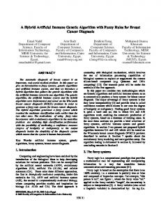
The GA decomposition sequence is shown in figure 1. initial status Time steps
hr. 1
GA run Including 11...01 in the new population
hr. 1 soln. hr. 2
create new offspring using selection, crossover and mutation operators
11...01
00...01
gen=gen+1
no
maximum generation yes
GA run Including
hr=hr+1 no
00...01 in the new population
yes last hour
stop
Fig. 2 Normal genetic algorithm cycle
START hr. 1 soln. hr. T
00...01
hr. T-1 soln. 11...11
GA run Including
hr=1
11...11 in the new population
hr=hr+1 Run the priority list heuristic algorithm Run normal GA including a copy of the priority list solution in the initial population
Fig. 1 Decomposed GA steps This method uses the previous interval’s solution as a member of the starting population in a current time step. This helps in the GA search by introducing useful building blocks because many units retain the same bit positions in any two neighbouring time intervals, due to the nature of the load profiles and the unit time linkage constraints. The flow charts for the GA and hybrid GA cycles are shown in figures 2 and 3 respectively.
no
Last hour ? yes Stop
Fig. 3 Hybrid genetic algorithm cycle
4
5 Simulation results
Table 2: Performance on 110 unit system
CPU Time on DEC Axp 4610 Processor (Minutes)
5.1 Experiments
The hybrid GA, normal GA and the priority list heuristic method has been applied to two test systems for a 24 hour schedule with quadratic fuel input / power output generator characteristics. A power system with 10 generators, taken from an EPRI [17] study and a sample network with 110 generators have been used as test systems. For the 110 unit system, the spinning reserve is required to cover the loss of the capacity of the largest committed unit.
Table 1: Performance on 10 unit system
0.23
Percentage Improvement over the Heuristic Priority List method
3.681
HYBRID GA
2
-3.29
0.26
7
-1.66
0.34
17
-0.43
0.53
35
0.16
0.46
90
0.36
0.49
180
0.50
0.51
A summary of the genetic algorithm control variables are included in the tables. The population sizes have been kept proportionally low to save on computation time. The truncation fitnes scaling [15] has been applied to the fitnes values to avoid premature convergence. The mutation rate is taken as 1/2N, where N is the number of units. These parameters are established after a number of simulations, guided by theoritical foundations of GA.
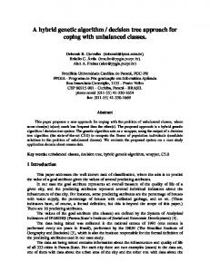
Tables 1 and 2 show the average percentage improvements of the GA and hybrid GA methods over the heuristic priority list method, for the 10 and 110 unit systems respectively. The plots are shown in figures 4 and 5 respectively.
NORMAL GA METHOD
NORMAL GA
GA parameters: population=110, pc=0.4, pm=0.005, Elite copies=10, stochastic remainder selection, uniform crossover
10 trials were carried out for each set number of generations, both for GA and the hybrid GA. Due to the stochastic nature of the GA method, the best result obtained should be chosen as the optimal schedule. The average performance is also computed to determine the reliability of the GA solutions.
CPU Time (sec.) on DEC Axp 4610 Processor
Percentage improvement over the heuristic priority list method
HYBRID GA METHOD
Normal GA
Hybrid GA
3.868
Percentage Improvement
0.38
3.846
3.920
0.63
3.920
3.966
0.87
3.960
3.978
1.16
3.966
3.978
4.00
1.41
3.978
3.978
1.68
3.978
3.978
2.03
3.978
3.978
2.35
3.978
3.978
2.62
3.978
3.978
3.95
3.90
3.85
3.80
3.75
3.70
GA parameters: population=30, pc=0.4, pm=0.05, Elite copies=1, stochastic remainder selection, uniform crossover
3.65 0.2
0.3
0.6
0.8
1.1
1.4
1.6
2.0
2.3
2.6
2.8
CPU Time Secs.
Fig. 4 Performance on 10 unit system
5
Hybrid GA
Normal GA
Production cost Percentage
Normal GA
Hybrid GA
Improvement
thousands
3960 1.00
3940 0.50
3920 0.00 -0.50
3900
-1.00
3880
-1.50
Best values
3860
-2.00
3840 -2.50
3820 -3.00
11
27
55
110
275
550
hundreds
-3.50
Function Evaluations 2.00
7.00
17.00
35.00
90.00
180.00
CPU time in minutes
Fig. 5 Performance on 110 unit system
Fig. 6 Normal GA and hybrid GA convergence characteristics on 110 unit system
5.2 Analysis of results
5.2.1 Comparison with other results
For 10 generators, the performance of the GA and the hybrid GA do not show any significant difference. Both perform better than the priority list method with a final improvement of 4 %, the hybrid algorithm providing better results in the initial stages of the trials. As the number of units increase, the GA performance initially starts off worse than the priority list, but as the number of generations, (CPU time) increases, it overtakes the priority list method. The hybrid method provides solution much earlier on in the run. On the 110 unit system, the hybrid GA achieves a 0.5 % improvement in solution within 17 minutes of cpu time while the normal GA gets to that solution after 3 hours. In the same system, the normal GA method overtakes the heuristic scheme after 35 minutes. It can be seen that a normal GA will finally arrive at a good solution, but the time it takes to reach the solution might not be within an acceptable limit for the scheduling problem. By combining the priority list method and exploiting the separable properties of the scheduling problem, good solutions can be obtained within reasonable times using a hybrid method.
Table 3 compares the solutions for the 10 unit test system with the results obtained using Lagrangian relaxation (LR) and Artificial neural network methods (ANN) [17]. The GA methods perform better than the ANN method and compares very favourably with the Langrangian relaxation method, it gives schedules within 0.2 percent of the langrangian relaxation method.
If the normal GA is left to run for long enough, in the end it will provide better solutions than the hybrid system as shown by the convergence characteristics in figure 6. The hybrid GA can sometime lead to a premature convergence as observed in figure 6.
Table 3: Comparison of schedule cost with LR and ANN methods ( 10 unit system ) METHOD
SCHEDULE COST ($)
Difference % with LR
LR
47,511
0.0
ANN
48,293
1.6
Hybrid GA
47,606
0.2
GA
47,606
0.2
Priority List
49,746
4.5
6 Conclusion The need for a hybrid system, becomes apparent as the system size is increased. The hybrid enables the GA to produce useful solutions within reasonable time limits. Using a fast heuristic method to provide domain knowledge can greatly enhance the performance of genetic algorithms whose main limitation is solution speed.
6
7 References
gorithms", IEE Proc. gen. transm. distrib., vol. 141, No. 5, Sept. 1994. 13. SHEBLE G. and MAIFELD T., "Unit commitment by genetic algorithm and expert system", Electric Power System Research 30 (1994) pp 115-121. 14. HOLLAND, J.H., "Adaptation in natural and artificial Systems", Ann Arbor: University of Michigan Press 1975. 15. GOLDBERG, D.E, "Genetic algorithms in search, optimisation and machine learning", Addision -Wesley, Reading 1989. 16. IRVING, M.R. and STERLING, M.J.H., " Economic dispatch of active power with constraint relaxation", Proc. IEE, pt. C, vol. 130, no. 4 July 1983, pp 172-177. 17. EPRI TR-103697 Technical report " Optimization of the unit commitment problem by a coupled gradient network and by a genetic algorithm, April 1994.
1. WOOD, A.J. and WOLLENBERG, B.F., "Power operation, generation and control", John Wiley and sons, 1984. 2. FAHD, G. and SHEBLE G., " Unit commitment literature synopsis", IEEE Trans. PWRS, vol. 9, Feb. 1994 pp 128-135. 3. KHODAVERDIA, E., BRAMELLAR, A. and DUNNET, R.M., "Semi rigorous thermal unit commitment for large scale electrical power systems", Proc. IEE C, vol. 133, No. 4, May 1986 pp 157-164. 4. LI, S. and SHAHIDEHPOUR, S.H., "Promoting the application of expert systems in short term unit commitment", IEEE Trans. PWRS, Feb. 1993, pp 287-292. 5. PANG, C.K., SHEBLE, G.B and ALBUYEH, F., "Evaluation of dynamic programming based methods and multiple area representation for thermal unit commitments", IEEE Trans. PAS, vol. 100, No. 3, March 1981, pp 1212-1218. 6. COHEN, A.I. and YOSHIMUA, M., "A branch and bound algorithm for unit commitment", IEEE Trans., vol. PAS-102, 1983, pp 444-451. 7. DILLON, T.,S., EDWIN, K.W., KOCHS, H.D. and TAUD, R.J., "Integer programming approach to the problem of unit commitment with probabilisitic reserve determination", IEEE Trans., vol. PAS 97, no 6, 1978, pp 2154-2166 8. ZHUANG, F. and GALIANA F.D., "Towards a more vigorous and practical unit commitment by langrangian relaxation", IEEE Trans. PWRS, vol. 3, May 1988 pp 763-770. 9. MUSOKE, H.S., BISWAS, S.K., AHMED E., CLIFF P. and KAZIBWE W., "Simultaneous solution of unit commitment and dispatch problems using artificial neural networks", Int. Jnl. of Electrical Power and Energy Systems, vol. 15, No. 3, 1993 pp 193199. 10. ZHUANG, F. and GALIANA, F., "Unit commitment by simulated annealing", IEEE Trans. PWRS , vol. 5, no. 1, Feb. 1990 pp 311-317. 11. MULLER, H. and PETRITSCH, "Genetic programming and simulated annealing for optimisation of unit commitment", 11th Power systems computations conference, 1993 pp 1097. 12. DASGUPTA, D. and McGREGOR, D.R., "Thermal unit commitment using genetic al-
7
8
9
10
11