The server for movies schedules with the rate-monotonic (RM) scheduling policy while the other does with the earliest deadline first (EDF) scheduling policy.
Scheduling System Verification Pao-Ann Hsiung, Farn Wang, and Yue-Sun Kuo Institute of Information Science, Academia Sinica, Taipei, Taiwan, ROC {eric,farn,yskuo}@iis.sinica.edu.tw
Abstract. A formal framework is proposed for the verification of complex realtime systems, modeled as client-server scheduling systems, using the popular model-checking approach. Model-checking is often restricted by the large statespace of complex real-time systems. The scheduling of tasks in such systems can be taken advantage of for model-checking. Our implementation and experiments corroborate the feasibility of such an approach. Wide-applicability, significant state-space reduction, and several scheduling semantics are some of the important features in our theory and implementation.
1 Introduction Model-checking has the promise of a formal, full, and automatic verification of complex industrial implementations in the future. In spite of the recent success in the formal verification of real-time systems, it is still quite infeasible to formally verify largescale real-world systems due to their high degree of complexity. On the other hand, engineers have developed various paradigms to help build and verify safer systems. One such paradigm is the scheduling paradigm which greatly simplifies the interaction among many processes to periodical and aperiodical computation time contention. But still, scheduling paradigm represents a too much simplified paradigm for many complex systems, such as protocol design, client-server systems, communication systems, . . .. In this paper, we construct a theoretical framework which combines the advantages of model-checking and scheduling paradigm with several concurrent scheduling servers employing different scheduling policies. Our implementation and experiments show its benefit and feasibility by comparing with a naive verification effort, that is, pure modelchecking approach. Experiment data shows that exponential reduction in state-space size can be reached. In our framework, a scheduling client-server system consists of a set of servers, with scheduling policies specified, and a set of scheduling client automata which are basically real-time automata extended with scheduling tasks specified at different modes. One major issue in such systems is the difficulty of compromising between two time scales : the job-computation time unit ∆J and the schedulability-check time unit ∆S . Usually ∆J is several orders of magnitude larger than ∆S . In real-time systems modelchecking, very often the time and space complexities are proportional to the timing constants used in the system description. With such a big disparity between ∆J and ∆S , the complexity of scheduling system model-checking can easily grow beyond manageable. In this work, we adopted the following technique. The systems will still be presented with time unit ∆J . But, when we are in a mode to check the schedulability, we shall W.R. Cleaveland (Ed.): TACAS/ETAPS’99, LNCS 1579, pp. 19–33, 1999. c Springer-Verlag Berlin Heidelberg 1999
20
Pao-Ann Hsiung, Farn Wang, and Yue-Sun Kuo
derive formulas, with respect to different scheduling policies, to calculate the computation time γS for the schedulability-check. Then the duration of the schedulability-check γ is set to be d ∆SJ e in the time unit of ∆J . With this technique, we can circumvent the potential combinatorial complexities caused by the disparity between the two time-scales. Another major issue is: when exactly should the checking for schedulability of the tasks in a mode be performed. Two alternatives arise here, namely, (1) checking before an in-coming transition of the mode is taken, or (2) checking after an in-coming transition of the mode is taken. Several different kinds of semantics related to schedulability checking are possible. These are discussed in subsection 3.1. Following is an example of a video system. Example 1. : Video System Here, we have two servers and two clients in a Video-on-Demand system illustrated in Fig. 1. The two clients issue task service requests to both the servers concurrently. The two servers check if requests are schedulable and then either acknowledge or reject the requests. The server for movies schedules with the rate-monotonic (RM) scheduling policy while the other does with the earliest deadline first (EDF) scheduling policy. The explanation of some popular scheduling policies can be found in section 2. The Movie Server stores a set of movie files ready for access by clients under the rate-monotonic scheduling policy. The Commercials Server stores a set of commercial files and work with the earliest-deadline first scheduling policy. As shown in Fig. 1, the clients are modeled by finite-state automata that are enhanced with clocks and scheduling tasks. In the figure, boxes represent different operational modes of the clients and the arrows represent transitions between modes. x and y are the two clocks used to control the operation times in the client automata. For example, the assignment x := 0 beside an arrow means that the clock x is reset to zero during the transition. The predicate x = 35 on an out-going transition in Client A means that the transmission of movie “Pretty Woman,” should end at 35 time units. Within each box, we specify tasks by a tuple (α, c, p, d, f ) where α is the server identification, c is the computation time of the task within each period, p is the period for the task, d is the deadline for each instance of a task, and f specifies if fixed priority (f = 1) or dynamic priority (f = 0) is to be used. It is important that at any instant of the computation, the tasks set admitted to each server remains schedulable. k The outline of this paper is as follows. Section 2 gives a brief survey of the priority scheduling policies used in our system. Section 3 presents the formal system model and describes how model-checking is used to verify the system. Section 4 describes our implementation of the model-checking approach using the popular HyTech tool and shows the benefit of our approach using some application examples. Section 5 concludes the paper. In the following, we use N and R+ to denote the set of non-negative integers and the set of non-negative real numbers.
2
Review of scheduling research
A real-time system generally needs to process various concurrent tasks. A task is a finite sequence of computation steps that collectively perform some required action
Scheduling System Verification S1
21
S2
Movie Server
Commercial Server Earliest Deadline First
Rate-Monotonic
Client A
Client B .... x .... ..
........... .
:= 0
.... y .....
Commercials
........... .
(S2 ; 5; 9; 9; 0)
= 38 x := 0
x
.... ....
� � 30
25 x x := 0
y y
= 22 := 0
:= 0
Commercials (S2 ; 1; 2; 2; 0)
.. .... .... .... y = .... .... .... y := 0 . . . . . . ......
10
...........
.... .... .... .... y > .... .... ..... ..........y
y
10 := 0
Pretty Woman
Batman II
Lion King
(S1 ; 2; 5; 5; 1)
(S1 ; 2; 5; 5; 1)
(S1 ; 1; 6; 6; 1)
Commercials
Commercials
Commercials
(S2 ; 2; 7; 7; 0)
(S2 ; 1; 9; 9; 0)
(S2 ; 3; 8; 8; 0)
= 35 x := 0
x .... ....
y .... y ....
= 12 := 0
y .... y ....
y
= 25 := 0
�
15 := 0
Peewee Herman
Terminator I
Toy’s Story
(S1 ; 2; 3; 3; 1)
(S1 ; 1; 4; 4; 1)
(S1 ; 1; 3; 3; 1)
Commercials
Commercials
Commercials
(S2 ; 1; 8; 8; 0)
(S2 ; 3; 7; 7; 0)
(S2 ; 2; 7; 7; 0)
Fig. 1. A video-on-demand system
of a real-time system and may be characterized by its execution time, deadline, etc. Periodic tasks are tasks that are repeatedly executed once per period of time. Each execution instance of a periodic task is called a job of that task. In a processor-controlled system, when a processor is shared between time-critical tasks and non-time-critical ones, efficient use of the processor can only be achieved by careful scheduling of the tasks. Here, time-critical tasks are assumed to be preemptive, independent, periodic, and having constant execution times with hard, critical deadlines. Scheduling may be time-driven or priority-driven. A time-driven scheduling algorithm determines the exact execution time of all tasks. A priority-driven scheduling algorithm assigns priorities to tasks that determines which task is to be executed at a particular moment. We mainly consider time-critical periodic tasks with the above assumptions and scheduled using priority-driven scheduling algorithms. Depending on the type of priority assignments, there are three classes of scheduling algorithms: fixed priority, dynamic priority, and mixed priority scheduling algorithms. When the priorities assigned to tasks are fixed and do not change between job executions, the algorithm is called fixed priority scheduling algorithm. When priorities
22
Pao-Ann Hsiung, Farn Wang, and Yue-Sun Kuo
change dynamically between job executions, it is called dynamic priority scheduling. When a subset of tasks is scheduled using fixed priority assignment and the rest using dynamic priority assignment, it is called mixed priority scheduling. Before going into the details of scheduling algorithms, we define the task set to be scheduled as a set of n tasks {φ1 , φ2 , . . . , φn } with computation times c1 , c2 , . . . , cn , request periods p1 , p2 , . . . , pn , and phasings h1 , h2 , . . . , hn . A task φi is to be periodically executed for ci time units once every pi time units. The first job of task φi starts execution at a time hi . The worst-case phasing called a critical instant occurs when all hi = 0, for all i, 1 ≤ i ≤ n. Liu and Layland [LL73] proposed an optimal fixed priority scheduling algorithm called the rate-monotonic (RM) scheduling algorithm and an optimal dynamic priority scheduling algorithm called earliest-deadline first (EDF) scheduling. The RM scheduling algorithm assigns higher priorities to tasks with higher request rates, that is, smaller request periods. Liu and Layland proved that the worst case utilization bound of RM was n(21/n − 1) for a set of n tasks. This bound decreases monotonically from 0.83 when n = 2 to loge 2 = 0.693 as n → ∞. This result shows that any periodic task set of any size will be able to meet all deadlines all of the time if RM scheduling algorithm is used and the total utilization is not greater than 0.693. The exact characterization for RM was given by Lehoczky, Sha, and Ding [LSD89], they proved that given periodic tasks φ1 , φ2 , . . . , φn with request periods p1 ≤ p2 ≤ . . . ≤ pn computation requirements c1 , c2 , . . . , cn , and phasings h1 , h2 , . . . , hn , φi is schedulable using RM iff Min{t∈Gi } Wi (t)/t ≤ 1
(1)
Pi where Wi (t) = j=1 cj dt/pj e, the cumulative demands on the processor by tasks over [0, t], 0 is a critical instant (i.e., hi = 0 for all i), and Gi = {k · pj | j = 1, . . . , i, k = 1, . . . , bpi /pj c}. Liu and Layland discussed the case when task deadlines coincide with request periods, whereas Lehoczky [L90] considered the fixed priority scheduling of periodic tasks with arbitrary deadlines and gave a feasibility characterization of RM in this case: given a task set with arbitrary deadlines d1 ≤ d2 ≤ . . . ≤ dn , φi isPRM schedulable iff Maxk≤Ni Wi (k, (k − 1)pi + di ) ≤ 1 where Wi (k, x) = mint≤x (( i−1 j=1 cj dt/pj e + kci )/t) and Ni = min{k | Wi (k, kpi ) ≤ 1}. The worst case utilization bound of RM with arbitrary deadlines was also derived in [L90]. This bound (U∞ ) depends on the common deadline postponement factor ∆, i.e., di = ∆pi , 1 ≤ i ≤ n. � U∞ (∆) = ∆loge
∆+1 ∆
� , ∆ = 1, 2, . . .
(2)
For ∆ = 2, the worst case utilization increases from 0.693 to 0.811 and for ∆ = 3 it is 0.863. Recently, the timing analysis for a more general hard real-time periodic task set on a uniprocessor using fixed-priority methods was proposed by H¨arbour et al [HKL94].
Scheduling System Verification
23
Considering the earliest deadline first dynamic priority scheduling, Liu and Layland [LL73] proved that given a task set, it is EDF schedulable iff n X ci ≤1 p i=1 i
(3)
and showed that the processor utilization can be as high as 100%. Liu and Layland also discussed the case of Mixed Priority (MP) scheduling, where given a task set φ1 , φ2 , . . . , φn , the first k tasks φ1 , . . . , φk , k < n, are scheduled using fixed priority assignments and the rest n − k tasks φk+1 , . . . , φn are scheduled using dynamic priority assignments. It was shown that considering the accumulated processor time from 0 to t available to the task set (ak (t)), the task set is mixed priority schedulable iff n−k X� t � (4) ck+i ≤ ak (t) pk+i i=1 for all t which are multiples of pk+1 or . . . or pn . Here, ak (t) can be computed as follows. � � k X t cj ak (t) = t − p j j=1 Although the EDF dynamic priority scheduling has a high processor utilization, in recent years fixed priority scheduling has received great interests from both academy and industry [LSD89, L90, SG90, HKL91, SKG91, TBW92, KAS93, HKL94]. Summarizing the above scheduling algorithms, we have five different cases of schedulability considerations: • RM-safe: all task sets are schedulable as long as the server utilization is below loge 2 = 0.693, • RM-exact: all task sets satisfying Equation (1) are schedulable, • RM-arbitrary: all task sets are schedulable as long as the server utilization is below ∆loge ((∆ + 1)/∆) (Equation (2)), • EDF: all task sets satisfying Equation (3) are schedulable, • MP: all task sets satisfying Equation (4) are schedulable,
3 Client-Server Scheduling System Model Modeling a real-time system as a client-server scheduling system, our target system of verification consists of a constant number m of servers that perform scheduling and a constant number n of clients that issue scheduling requests. A server adopts a scheduling policy. Each client is modeled with a client automaton such that the client issues different scheduling requests in various modes. On receiving a request for scheduling a set of tasks, a server decides whether the tasks are currently schedulable or not. Definition 1. : A Periodic Task A periodic task is a tuple φ = (α, c, p, d, f ), where α is the identification of the server on which the task is to be processed, c is the constant computation time of a job, p is the
24
Pao-Ann Hsiung, Farn Wang, and Yue-Sun Kuo
request period of a job, d is the deadline within which a job must be completed before the next job request occurs, and f specifies if the task must be scheduled using fixed priority or dynamic priority, that is, f = 1 for fixed priority and f = 0 for dynamic priority, c ≤ p, c ≤ d, and c, p, d ∈ N , the set of nonnegative integers. k Notationally, we let TH be the universal set containing all possible tasks in a system H. We model the behavior of clients with timed automata which are automata enhanced with clocks. It is assumed that the current mode of each client is broadcast to all the clients in the same system. The behavior of a client in each mode can be expressed through a state predicate, which is a combination of propositions and timing inequalities on clock readings. Given a set of propositions P and a set of clocks X, a state predicate η of P and X has the following syntax. η ::= false | r | x ∼ a | x + a1 ∼ y + a2 | η1 ∧ η2 where r ∈ P , x, y ∈ X, a, a1 , and a2 are rational numbers, ∼ ∈ {≤, }, and η1 , η2 are state predicates. Let B(P, X) be the set of all state predicates on P and X. Given a set of propositions P and a set of clocks X, a client is modeled as follows. Definition 2. : Client Automaton (CA) A Client Automaton (CA) is a tuple C = (M, m0 , P, X, χ, µ, E, ρ, τ ) with the following restrictions. • M is a finite set of modes. • m0 ∈ M is the initial mode. • P is a set of atomic propositions. • X is a set of clocks. • χ : M 7→ B(P, X) is a function that labels each mode with a condition true in that mode. • µ : M 7→ 2TH maps each mode to a finite subset of tasks in TH . • E ⊆ M × M is the set of transitions. • ρ : E 7→ 2X maps a transition to a set of clocks that are reset on that transition. • τ : E 7→ B(P, X) maps each transition to a triggering condition. k The CA C starts execution at its mode m0 . We shall assume that initially, all clocks read zero. In between transitions, all clocks increment at a uniform rate. The transitions of the CA may be fired when the triggering condition is satisfied. Definition 3. : Servers A server is a tuple hα, φi where α is the unique identification for the server and φ is the scheduling policy of the server. k Now with a set of servers, a set of client automata, and the ratio between the schedulability-check time unit and the job-computation time unit, we are ready to define what is a scheduling system. Definition 4. : Scheduling systems A scheduling system H is defined as a tuple ({S1 , S2 , . . . , Sm }, {C1 , C2 , . . . , Cn }, P, X, Γ ), where {S1 , S2 , . . . , Sm } is a set of servers, {C1 , C2 , . . . , Cn } is a set of client automata, P , and X are respectively the set of atomic propositions and the set of clocks used in C1 , . . . , Cn , and Γ is a ratio of a schedulability-check time unit to a job computation time unit. k
Scheduling System Verification
25
Definition 5. : States and their admissibility Given a system H = ({S1 , . . . , Sm }, {C1 , . . . , Cn }, P, X, Γ ) with Ci = (Mi , m0i , P, X, S χi , µi , Ei , ρi , τi ), a state s of+H is defined as a mapping from {1, ..., n} ∪ P ∪ X to 1≤i≤n Mi ∪ {true, false} ∪ R such that • ∀i ∈ {1, ..., n}, s(i) ∈ Mi is the mode of Ci in s; • ∀r ∈ P , s(r) ∈ {true, false} is the truth value of r in s; and • ∀x ∈ X, s(x) ∈ R+ is the reading of clock x in s. Further, a state s is said to be admissible when: V • s |= 1≤i≤n χi (s(i)), and k • the task set ∪1≤i≤m µi (s(i)) ⊆ TH at s is schedulable by the servers. Definition 6. : Satisfaction of state predicate by a state State predicate η is satisfied by a state s, written as s |= η iff • s 6|= false; • ∀r ∈ P, s |= r iff s(r) = true; • ∀x ∈ X, s |= x ∼ a iff s(x) ∼ a; • ∀x, y ∈ X, s |= x + a1 ∼ y + a2 iff s(x) + a1 ∼ s(y) + a2 ; and • s |= η1 ∧ η2 iff s |= η1 and s |= η2
k
Definition 7. : Mode Transition Given a system H = ({S1 , . . . , Sm }, {C1 , . . . , Cn }, P, X, Γ ) with Ci = (Mi , m0i , P, X, χi , µi , Ei , ρi , τi ), and two states s and s0 , there is a mode transition from s to s0 in H, in symbols s → s0 , iff • both s and s0 are admissible states, • there is an 1 ≤ i ≤ n such that - (s(i), s0 (i)) ∈ Ei ; - s(i) |= τi (s(i), s0 (i)); - for all 1 ≤ j ≤ n and j 6= i, s(j) = s0 (j); - ∀x ∈ X ((x ∈ ρi (s(i), s0 (i)) ⇒ s0 (x) = 0)∧(x 6∈ ρi (s(i), s0 (i)) ⇒ s0 (x) = s(x))). k Given a state s and a δ ∈ R+ , we let s + δ be the state that agrees with s in every aspect except for all x ∈ X, s(x) + δ = (s + δ)(x). 3.1 Semantics of Schedulability Checking The admissibility of a new state, that is, the schedulability check, can be implemented in either one of two ways: (1) checking before transition, and (2) checking after transition. In the former case, when a client is in a particular mode (may be executing some tasks) and an out-going transition is enabled, it must first check with the servers by sending scheduling requests before the out-going transition is taken. In the latter case, when a client is in a particular mode and an out-going transition is enabled, the client may take the transition and then check if the tasks in the new mode are schedulable. (a) Scheduling-Check Before Transition (SCBT): The semantics here differ mainly in the duration time that a client automata can stay in a mode. Here, we propose three possibilities.
26
Pao-Ann Hsiung, Farn Wang, and Yue-Sun Kuo
• (SPR) Saturated Parallel Request: If more than one out-going transitions of the currently executing mode are concurrently enabled, then the client keeps on issuing scheduling requests to all servers according to its next-states task sets. Once a positive response is back for any one next-state, the client can make the corresponding transition. If more than one positive responses are received, the client makes all corresponding transitions in parallel (parallelism is implemented as interleaving of transition sequences). In this semantics, the duration time of a mode must be greater than the schedulability-check computation time for the corresponding next state. This semantics needs minimal modification to translate to HyTech input form. • (SQR) Sequential Request: The client nondeterministically chooses a next state and posts requests to the servers specified in the task set of the next state. No request to any server will be issued until the last request is replied. In this semantics, the client nondeterministically chooses a next-state and polls the servers for schedulability-check. Only after response is back, the client may test for another next-state. Thus the duration time a client can stay in a mode must be the sum of a sequence of schedulability-check computation times. • (NPR) Non-saturated Parallel Request: The client polls all the servers for all its next-states. Once a reply is back, the client choose between taking the corresponding transition or not. If it does not transit at the moment, then it issues another schedulability request for the same next-state. In this semantics, the duration time must be at least a multiple of the schedulability-check computation time for a particular next-state. (b) Scheduling Check After Transition (SCAT): In this case, modularity of the system specifications is preserved and transitions occur according to the timed automata semantics. Scheduling systems implemented using this scheme of schedulability checking have two semantics related to scheduling, that is strict scheduling semantics and loose scheduling semantics. • (SSS) Strict Scheduling Semantics: In a particular mode, it may happen that the specified task set cannot be scheduled before an out-going transition is enabled. In this situation, when we do not allow the client to make the enabled transition from the non-scheduled mode, we call it strict scheduling semantics. • (LSS) Loose Scheduling Semantics: In a specific mode, when the specified tasks are not scheduled (i.e., schedulability-check returns negative response) before an out-going transition is enabled, the client may choose to either keep on issuing scheduling requests for non-scheduled tasks set or transit to the next mode by making the enabled transition. This is called loose scheduling semantics and results in a larger global state space as shown by examples in Section 4. The computation of our scheduling system is defined in the following. Definition 8. : s-run Given a system H and a state s of H, a computation of H starting at s, called an s-run, is a sequence ((s1 , t1 ), (s2 , t2 ), . . . . . .) of pairs such that • s = s1 ; and • for each t ∈ R+ , ∃j ∈ N such that tj ≥ t; and
Scheduling System Verification
27
• for each integer j ≥ 1, for each real 0 ≤ δ ≤ tj+1 − tj , sj is admissible and sj + δ |= χi (sj (i)); and • for each j ≥ 1, H goes from sj to sj+1 because of - mode transition, i.e. tj = tj+1 ∧ sj → sj+1 ; or - time passage, i.e. tj < tj+1 ∧ sj + tj+1 − tj = sj+1 . • The duration time a client can stay in a mode must satisfy the chosen semantics. k
4 Implementation The theoretical framework of a Client Server Scheduling System Model as presented in Section 3 has been implemented into a practical tool for verifying scheduling systems. The implementation mainly constitutes two parts: scheduling check time computation and translating a scheduling system description into a pure timed automata specification. The resulting timed automata specification can be seen as a special case of linear hybrid automata, hence the popular tool called HyTech is used for verifying our resultant system descriptions. The two semantics of scheduling check before and after transition have both been implemented into our translator tool. Experiments have been conducted with several application examples from both hardware and software. Though the degree of advantage in using our proposed approach for verifying scheduling systems vary, yet all of the examples show an appreciable amount of decrease in the size of the reachable state space required for verification. 4.1 Scheduling Check Time Computation Before entering a state s, a system must check with the servers if it is an admissible state, that is, if all the tasks (∪vi=1 µi (s(i))) in that state are schedulable by the servers. This computation for schedulability check is done exclusively by each client by locking the servers and requires a small period of time which depends on the scheduling algorithms used by the servers. Usually the computation for schedulability check is a very small one compared to the scheduled job computation time. However, as the number of contending processes increases, some scheduling policies may consume an amount of time that cannot be considered negligible. For example, for a 200 MHz CPU, the processor cycle time is around 5 × 10⁻⁸ seconds, and considering a single instruction to be 2 cycles, the CPU requires only 10−7 seconds for one processor operation. At the same time, one tick of scheduled job computation time in a real-time system is usually in the order of a millisecond (ms). Hence, the ratio of a server cycle time to a job computation time unit is 10−4 . Normally, a task set size in a real-time system is in the order of 10 to 100. A schedulability-check time linear in the size of the task set would be negligible compared to the computation time of the task set, but if it is quadratic, it would be in the order of one job time unit. For analyzing the amount of time required for schedulability-check, we define the set of tasks in some state s, which are to be scheduled on some particular server Sk using some scheduling algorithm Rk , 1 ≤ k ≤ m. νs (Rk ) = {φ | φ = (Sk , c, p, d, f ), φ ∈ µi (s(i)), 1 ≤ i ≤ n}
(5)
28
Pao-Ann Hsiung, Farn Wang, and Yue-Sun Kuo 4
3.5 others: RM_safe, RM_arb, ED
schedulability check time (s)
3
2.5 RM_exact 2
1.5 MP 1
0.5 others 0 -6 10
-5
-4
-3
10 10 10 processor operation time to computation time unit ratio (log)
10
-2
Fig. 2. Schedulability Check Time The schedulability check time required for each of the five variations of priority scheduling described in section 2 using different ratios of server operation time to computation time unit is illustrated in Fig. 2. We observe that the schedulability check time is negligible when the ratio is of the order of (10−4 ). We make the following assumptions: • The execution of all jobs of each task start at integer-valued time instants. • A schedulability check is assumed to take 1 computation time unit when it is not greater than 1 unit and it is taken as 2 time units when it is between 1 and 2, that is, the schedulability check time is taken as the next larger integer if it is not already an integer. As far as RM-safe, RM-arbitrary, and EDF priority scheduling are concerned, the schedulability check time only depends on the total utilization of a server. � As long as , and 100%, the utilization is below the respective bounds of n(21/n − 1), ∆loge ∆+1 ∆ all tasks of all phasings, request periods, and deadlines can be scheduled. This check requires time linear in |νs (R)|, where R is RM-safe, RM-arbitrary, and EDF, respectively. Hence, assuming the ratio of a processor operation time to a job computation time unit to be top , for example, top is in the order of 10−4 for a 200 MHz CPU and a 1 ms tick computation time, the time spent for checking schedulability of RM-safe, RM-arbitrary, and EDF by a particular server are as follows. γs (RMsaf e ) = |νs (RMsaf e )| × top
(6)
γs (RMarb ) = |νs (RMarb )| × top
(7)
γs (EDF ) = |νs (EDF )| × top
(8)
For RM-exact (Equation 1) scheduling, the schedulability check time is as follows. γs (RMexact ) = |νs (RMexact )|2 × p|νs (RMexact )| × top
(9)
Scheduling System Verification
29
where p|νs (RMexact )| is the largest period in νs (RMexact ). As for mixed priority scheduling, the schedulability check time is as follows. γs (M P ) = |νs (M P )| × LCM{pk | φ = (S, c, pk , d, 1)} × top
(10)
where LCM is the least common multiple and φ(S, c, pk , d, 1) is a task in state s, which is to be scheduled using dynamic priority. Hence, the total time spent on schedulability check during a state transition to a state s in a system H = (hS1 , S2 , . . . , Sm i, hR1 , R2 , . . . , Rm i, hC1 , C2 , . . . , Cn i, P, X, TH , top ) is as follows. γs = Max1≤k≤m γs (Rk )
(11)
where Rk ∈ {RMsaf e , RMexact , RMarb , EDF, M P }. The difficulty in implementing scheduling check time computation lies in the fact that for RMexact and M P scheduling policies, the periods of all the currently executing tasks must be known (refer to Equations (10) and (11)), hence we must consider all possible permutations of the client modes for a complete check time computation. This also implies that the mode status of each client must be broadcast to all the other clients in the scheduling system. This broadcast has been implemented in our translator. 4.2 Translator We developed a translator for translating the client-server scheduling system specification (in our own input language) to the HyTech specification. Although a scheduling system can be specified using the HyTech input language, yet the specification would be very lengthy, tedious, and error-prone. Using our input language, the specification is short and compact and the translation is done systematically, thus avoiding any humanerrors. For example, in the real-time operating system example (described in subsection 4.3), using our input language the specification consisted of only 12 modes and 17 transitions, whereas the resulting translation into HyTech input language consisted of 58 modes and 416 transitions. Thus, the translator is a necessity for verifying scheduling systems. HyTech [HHWT95] is a popular verification tool for verifying systems modeled as linear hybrid automata. HyTech has been used to verify various different systems such as gas burner, railroad crossing controller, Corbett’s distributed controller, and protocols such as Fischer’s mutual exclusion protocol. Each client automaton is implemented as a linear hybrid automaton in HyTech and the analysis tool is used to verify our system. According to the different scheduling semantics, we have different types of implementation schemes. For the scheduling check before transition (SCBT) semantics, we have a transition-oriented implementation and for the scheduling check after transition (SCAT), we have a mode-oriented implementation. SCBT Implementation As illustrated in Fig. 3, each mode in the scheduling system description is implemented as a simple job execution location called RunJobs, but each mode transition is implemented as a set of three interconnected locations called Lock,
30
Pao-Ann Hsiung, Farn Wang, and Yue-Sun Kuo
M1
................................ ...... .... .... .. . ..... ... .... .... ..... ..................................
RunJobs
M1
.................................... ................ ....... ....... ..... ..... .... ... .. ... . .. ... ... ..... ... . . . ...... ...... .......... . . . . . . . . . . ........................................
trigger assignments pp p pp p pp pp pp pp pp pp pp pp pp p ppppp pppp p
M2
................................. ................. ........ ....... ..... ..... .... .... .. .. . .. ... .. ..... ... ...... ..... . . . . . .......... . .................................................
trigger pp p pp pp pp pp pp ppp pp pp pp p pp ppp pppp pppp p
ppppppppppp ppppppppppp ppppppppppp pppppppppp pp pppppppppp ppppppppppp ppppppppppp pppppppppp
............................... ...... .... ... .... ..... .. .... .. ...... .... ................................ .. ................. . . . . . .. ....... ...... . . . . . . . . ....... . ... ....... ...... ....... ...... ........ ......... ........ ....................... ....... . . . . . . . . . . . . . . . . . ...... .... ... .... ..... . ................................ .. ...... .... .. ..... ................. ... .. .... . .. . . . . . . . . ...... . ... .. ..................p............... . ... . ...... ppp ppp ...... . . . . . . . ppp . . . . . . . . . . . . . . . . . . . . . . p
l=0 l := i;
Sched Check
l i l
Lock
l=i
not schedulable
l := 0;
Error
ppp ppp ppp ppp ppp ppp ppp ppp ppp ppp ppp ppp ppp ppp pppp ppp ppp ppp ppp pppp ppp ppp pppp ppp pppp p ppp pp pp p pppp pppppp pppp pppp ppp pp ppppp ppp p pppppppppp ppppppppppp ppppppppp pp
= schedulable := 0;
M2
assignments
................................ .... ...... ... .... ... ... ... RunJobs .. .... .... ....... .............................
Fig. 3. Scheduling-Check Before Transition Implementation
SchedCheck, and Error. The purpose of these locations are, respectively, the locking of the servers, the checking for schedulability of the tasks in the next mode (the destination mode of the transition under consideration), and the resetting of internal variables when a negative response is received in SchedCheck. There is a location transition from Runjob to Lock and one from SchedCheck (on a positive response from the servers) to the RunJobs location of the destination mode. The triggering condition and the assignment statements of the transition under consideration are attached to the location transition from RunJobs to Lock and to the location transition from SchedCheck to next mode RunJobs location, respectively. The locking mechanism is similar to that for SCAT and is described in the SCAT implementation. Saturated parallel request (SPR) of SCBT requires the least modification with respect to HyTech, so only SPR was implemented. SCAT Implementation Each mode of a client automaton is implemented by four locations, namely, Lock, SchedCheck, RunJobs, and Error. A client must check the admissibility of a mode before entering it, and this check must be done exclusively by a client because otherwise the schedulability check performed will not be consistent. To ensure exclusiveness of schedulability check, we employ a simpler version of the Fischer’s mutual exclusion protocol [L87] and a lock (l) semaphore variable. Before performing schedulability-check, a client obtains ownership of l by setting l to its identification number so that it can exclusively do the checking. A client waits in location Lock for l to be free (i.e., l = 0) and when free, it sets l to its identification number. Schedulability check is done in the location SchedCheck if l is still set to its own identification number, otherwise the client returns to the location Lock. After schedulability check, the client
Scheduling System Verification
M1
.............................. ....... .... ....................................................... .... ...... ............ .. ..... . . .. ..... ... .... .... .... ...... .... ................................. .... ... .. ... ... ...... .. ..... ... . .. .................................. . . . . . ... .... .... .. .. . .. . . . . ... .... ... .. . ....... . . . . . . ............................ . . . . . . . . .... ......... ... ..... .... .... ..... ... ..... ..... ... ...... ......... .... .. .......... ....... ............... ... . . . . . . . . . . . . . . . . . . . . . . . . . . . . . . . . . . . ........ ....... .... . ..... ..... ..... ...... ..... ...... ... .... .. ..... ... . ... ................ .. . ... ..RunJobs . ... ... .... ....... ..... .... ...... ..... . ........... . . . ................................ . . . . . .............. .... .... .... .... .... .... .... .... .... .... .... ..... ............. . ............................... ....... .... .......................................................... . . . .......... ...... .. . .. ..... . ... . .... .... ... .... ....... .... .... .............................. .... ... .. .. .. ... ..... ... ....... .. ............................ . . . . . .. . ..... ..... . . . . ... .. . ... . .. . ... .. .. . ..... . . . . . ............ ................. .. . . . . . . . . . . .... ........ .. ..... ..... ... ..... ..... .. .... ..... .... ........ ...... ............ .... .............. . . . . . . . . ...... .. ............................... ............ ............... ....... ..... .... ..... ... ..... .... .. ... .. . ... ................. . ... ....RunJobs . ..... ... .. ... ... ..... ...... .... ............ ................. ................................. .........
l=i l := 0;
schedulable
Lock
l=0 l := i; Sched Check l=i not schedulable l := 0;
M1
M2
l=i l := 0;
schedulable
mode transition
Lock
l=0 l := i; Sched Check l=i not schedulable l := 0; Error
Fig. 4. SCAT: SSS Implementation
.................................. . ........................................ .... ............ ...... ....... ..... ... ......... ..... .... .. ..... .... .... .... ...... .... .................................. ... ... .. ... ... ...... .. ..... ... ............................ . .. . . . . . ..... .. ..... . . . . . ... .... ... . ... ... ... ..... . . . . . . ........... ................. .. . . . . . . . . . . .... ........ .. ..... ..... .. .... .. ..... ..... ..... ... ...... . .... ................. ... ............... . . . . . . . . . . . . . . . . . . . . . . . . . . . . . .......... . ....... ........ .............. ..... ..... ...... .... ...... ... ..... .... ... ... ... ...... .... ...RunJobs . ............. .. ... ... ....... ..... ..... .... .... . . ........... ............ ............... . . . . . ................. ........... .... ... .... ... .... ... .... ... .... ... .... . .... .. .... ... .... .. .... .. .... ... ...... ...... . ................. .. ............................... ....... .... .......................................................... .... .......... ...... . ..... ..... .... ... ... .... ... ..... .... ........... ................. .... ......... ... .. .. .. ..... ... ... ...... .. ........................ . . . . . . . . .. ..... ... ... .... . ... .. . .... . ... .... .. . . .. . . ....... . .. ................................. . . .. .... ........ . . . . . . . ..... . ..... ..... ... ..... ..... ..... .... . ........ ................. .... ........... .. .... .... ................................ .................................. . . . . . . . . . . . . . . .... .... .. .. ...... ... ... .. .. ........ ...RunJobs ... . ... ................ ... ... ..... ..... ... ..... ......... ............ ................ ........................ .........
l=i l := 0;
schedulable
Error
31
Lock
l=0 l := i; Sched Check l=i not schedulable l := 0; Error
M2
l=i l := 0;
schedulable
mode transition
Lock
l=0 l := i; Sched Check l=i not schedulable l := 0; Error
Fig. 5. SCAT: LSS Implementation
changes mode in location SchedCheck and if schedulable the jobs of the scheduled tasks are executed in location RunJobs, otherwise the location Error is entered. As illustrated in Fig. 4, in the case of strict scheduling semantics (SSS), the location Error has only one out-going transition to location Lock since the tasks must be scheduled and executed in the mode before any mode transition occurs. The location transition from RunJobs to Lock implements a mode transition in the client automaton. As illustrated in Fig. 5, in the case of loose scheduling semantics (LSS), the location Error has two out-going transitions: one to the location Lock of the current mode (just as in the case of strict scheduling semantics) and one to the location Lock of the next mode. The two location transitions from location Error to the two Lock locations implement a mode transition. 4.3 Application Examples To illustrate the generality of our approach, we demonstrate the benefits of three different types of systems: a hardware system such as a video-on-demand (VOD) system, a software system such as a real-time operating system (RTOS), and an agent system such as a package delivery system (PDS). There are two servers in the video examples (just as in Fig. 1). The movie server schedules tasks with the rate-monotonic (safe) policy, while the commercial server does so with the earliest-deadline first policy. For the real-time OS example, there are four servers: OS kernel, display, memory, and printer, which use rate-monotonic (safe),
32
Pao-Ann Hsiung, Farn Wang, and Yue-Sun Kuo
Table 1. Comparison of Pure Model Checking and Our Approach Specifications Example VOD(Fig. 1) VOD1 VOD2 RTOS1 RTOS2 PDS1 PDS2
|S| |C| 2 2 2 4 4 3 3
2 3 3 3 3 4 4
Number of regions (convex predicates) SCBT SCAT | ∪ Mi | | ∪ Ei | SPR SSS LSS PM C SM C % PM C SM C % PM C SM C 8 9 139 90 64.7 110 68 61.8 120 78 6 7 344 231 67.2 141 92 65.2 147 98 9 11 114 46 40.3 80 34 42.5 107 61 11 14 2962 2247 75.9 1980 1486 75.0 2054 1560 12 16 830 306 36.9 684 256 37.4 728 300 6 6 4717 3708 78.6 2114 1610 76.1 2140 1636 6 6 3306 1554 47.0 1193 536 44.9 1204 547
% 65.0 66.7 57.0 75.9 41.2 76.5 45.4
S: set of servers, C: set of clients, | ∪ Mi |: total #modes, | ∪ Ei |: total #transitions PM C : Pure Model Checking, SM C : Scheduling System Model Checking, %: SM C / PM C
earliest-deadline first, rate-monotonic (arb), rate-monotonic (exact) policies, respectively, for scheduling the tasks. For the delivery system example, it is assumed that there are three delivery agents and four clients. The delivery agents must deliver packages to the clients according to scheduling policies: rate-monotonic (exact), earliest-deadline first, and mixed scheduling. Two versions are given for each of the three kinds of systems. All the six examples were specified in our input language which was then automatically translated by our translator into the HyTech input language. The results, as tabulated in Table 1, show that our approach indeed reduces the total size of the system state space for verification as compared to the pure model checking approach. Here, pure model checking means that we do not take advantage of the scheduling algorithms and directly verify the systems which might contain a lot of unschedulable states. Drastic reductions can be achieved in systems that have a heavy workload. With each type of example, either VOD or RTOS, it is observed that with a high complexity in the client automata (i.e., the number of modes and transitions) the SCBT implementation shows a larger benefit (i.e., a smaller state space size) compared to all the semantics of the SCAT implementation. This is due to the stronger semantics of a transition not occuring before the tasks schedulability of its destination mode is checked. Comparing the two semantics of SCAT: SSS and LSS, in all the examples it is observed that strict semantics shows a larger benefit with our approach. This is due to the stronger restriction in SSS of tasks required to be scheduled before the client can progress on. Thus, we can conclude that both theoretically and experimentally we have shown that SCBT has the strongest notion of schedulability and LSS of SCAT has the weakest notion with SSS of SCAT in-between SCBT and LSS.
5 Conclusion Model-checking, though a popular verification method, has yet to be made more efficient for verifying the current highly complex systems. We have shown how complex
Scheduling System Verification
33
real-time systems can be easily verified using the popular model-checking approach if we model the complex system as a client-server scheduling system and then verify it. This approach is meaningful when we observe that almost all complex systems need some sort of scheduling so that the tasks can be executed consistently and efficiently. Our preliminary effort has been shown feasible through the implementation using our translator and the HyTech verification tool. Different semantics have been implemented and compared using several examples. Our future work will include the development of a tool devoted to the verification of such systems using symbolic model checking.
References [ACD90]
R. Alur, C. Courcoubetis, and D.L. Dill, “Model checking for real-time systems,” 5th IEEE LICS, 1990. [CES81] E.M. Clarke, E.A. Emerson, and A.P. Sistla, “Automatic verification of finite state concurrent system using temporal logic,” Procs. Workshop on Logics of Programs, Lecture Notes in Computer Science, vol. 131, pp. 52–71, 1981. [E90] E.A. Emerson, “Temporal and Modal Logic,” in Handbook of Theoretical Computer Science, Ed. J. van Leeuwen, Elsevier Science Publishers B.V., 1990. [HHWT95] T.A. Henzinger, P.-H. Ho, and H. Wong-Toi, “HyTech: the next generation,” Procs. IEEE Real-Time Systems Symposium, pp. 56–65, 1995. [HKL91] M.G. Harbour, M.H. Klein, J.P. Lehoczky, “Fixed priority scheduling of periodic tasks with varying execution priority,” Procs. IEEE Real-Time System Symposium, pp. 116–128, 1991. [HKL94] M.G. Harbour, M.H. Klein, J.P. Lehoczky, “Timing analysis for fixed-priority scheduling of hard real-time systems,” IEEE Trans. Software Engineering, vol. 20, no. 1, Jan. 1994. [KAS93] D.I. Katcher, H. Arakawa, and J.K. Strosnider, “Engineering and analysis of fixed priority schedulers,” IEEE Trans. Software Engineering, vol. 19, pp. 920–934, Sept. 1993. [L87] L. Lamport, “A Fast Mutual Exclusion Algorithm,” ACM Trans. on Computer Systems, vol. 5, no. 1, pp. 1–11, Feb. 1987. [L90] J.P. Lehoczky, “Fixed priority scheduling of periodic task sets with arbitrary deadlines,” Procs. IEEE Real-Time Systems Symposium, pp. 201–209, 1990. [LL73] C.L. Liu and J.W. Layland, “Scheduling algorithms for multiprogramming in a hard-real-time environment,” Journal of the Association for Computing Machinery, vol. 20, no. 1, pp. 46–61, Jan. 1973. [LSD89] J.P. Lehoczky, L. Sha, and Y. Ding, “The rate monotonic scheduling algorithm: exact characterization and average case behavior,” Procs. IEEE Real-Time Systems Symposium, pp. 166-171, 1989. [SG90] L. Sha and J.B. Goodenough, “Real-time scheduling theory and Ada,” IEEE Computer, vol. 23, pp. 53–62, Apr. 1990. [SKG91] L. Sha, M.H. Klein, and J.B. Goodenough, “Rate monotonic analysis for real-time systems,” Foundations of Real-Time Computing: Scheduling and Resource Management, A. van Tilborg and G.M. Koob, Eds. New York: Kluwer, pp. 129–155, 1991. [TBW92] K.W. Tindell, A. Burns, and A.J. Wellings, “Mode changes in priority pre-emptively scheduled systems,” Procs. IEEE Real-Time Systems Symposium, pp. 100–109, 1992.
10.1007/b107031130002