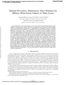
operational costs. This paper introduces a formal model of wind farm maintenance, and proposes ... multiple optimization criteria, including the leveled load of.
Scheduling the Maintenance of Wind Farms for Minimizing Production Loss Andr´ as Kov´ acs ∗ G´ abor Erd˝ os ∗ L´ aszl´ o Monostori ∗,∗∗ Zsolt J´ anos Viharos ∗ ∗
Computer and Automation Institute, Budapest, Hungary (e-mail: {andras.kovacs,gabor.erdos,laszlo.monostori,zsolt.viharos}@sztaki.hu) ∗∗ Budapest University of Technology and Economics, Hungary Abstract: With the extensive and worldwide increase of the market share of wind energy, the optimal operation of wind farms gains an ever growing significance. The planning and scheduling of maintenance operations is both decisive for turbine availability and a key component of the operational costs. This paper introduces a formal model of wind farm maintenance, and proposes a mixed-integer programming formulation for the problem of optimizing detailed maintenance schedules. Initial results are presented and directions for future research are pointed out. Keywords: wind energy, power plants, maintenance, scheduling, optimization, mathematical programming 1. INTRODUCTION Wind energy industry has experienced an extensive and worldwide growth during the past years. Certain forecasts indicate that the share of wind in Europe’s energy production will reach up to 20% in the close future (Blanco, 2009). Given these tendencies, the optimal operation of installed turbines has an ever increasing significance. Among operational decisions, the planning and scheduling of maintenance tasks is decisive both regarding turbine availability and operational costs. Maintenance scheduling will receive even more emphasis with the spread of offshore installations, whose operational cost is estimated to be 50% higher than for onshore farms (Markard and Petersen, 2009). Maintenance scheduling is not only an important, but also a complex problem. Schedulers must consider aspects like weather conditions, the availability of skilled technicians, expensive hired services (e.g., cranes or special trucks) and spare parts, as well as different kinds of interrelations of maintenance tasks. Moreover, the scheduler must adapt quickly to changing circumstances, such as newly detected failures or changes of the weather conditions. Finding optimal maintenance schedules is hence a challenging problem, and decision support from an automated scheduling system that is able to consider all the above aspects would be highly valuable. This paper presents the requirements for the maintenance schedule from the point of view of a wind farm operator, who is interested in maximizing the total energy produced, or in other words, minimizing the production loss. A formal mathematical model is introduced, and a mixed-integer programming (MIP) formulation is proposed. Initial experiments show that solving this MIP by a commercial solver results in close-to-optimal maintenance schedules. We note that the figures presented in the paper are used for demonstration only, and do not coincide with real-life data.
2. LITERATURE REVIEW Mathematical models and optimization methods for planning and scheduling maintenance operations have been widely studied for various application areas in production and in the service industry (Budai et al., 2008). Recent contributions include Davenport (2010), who presents an approach to scheduling the maintenance tasks in a semiconductor fabrication plant. The model takes into account the predicted production level over time, as well as the different skills and availability of technicians. It considers multiple optimization criteria, including the leveled load of technicians, the minimal disruption caused in production, and a quality measure of the timing of the individual maintenance tasks. Perron (2010) proposes a decomposition approach to a problem of scheduling teams of skilled workers for tasks to be performed at different locations. The problem is separated to a planning part (the formation of teams), solved by mixed-integer programming, and a detailed scheduling part (fixing the execution time of the tasks), solved by constraint programming. A closely related problem, where the emphasis is on the assignment of appropriate skilled workforce, is the audit scheduling or staff scheduling problem (Ernst et al., 2004). On the other hand, the literature of planning and scheduling maintenance specifically for wind turbines is rather scarce. The optimization of (periodic) preventive maintenance policies and the planning of maintenance activities are typically based on the generic models, see, e.g., (Scarf et al., 2005). The possibilities of applying condition monitoring systems and condition-based maintenance policies to wind turbines received significant attention recently. The technological and economical effects of the application of such systems and policies are analyzed by simulation experiments in (McMillan, 2008). The use of condition monitoring systems for both continental and offshore turbine farms is evaluated by life-cycle cost analysis on real data in (Nilsson and Bertling, 2007). Nielsen and Sorensen (2011)
developed optimal inspection and maintenance policies for offshore wind turbines using Bayesian decision theory. The approach is able to incorporate information coming from condition monitoring systems, and takes into account the uncertainty of the observed state of the critical components. 3. PROBLEM DEFINITION In this section we present in detail the maintenance processes at wind farms, as well as the resulting requirements for an automated maintenance scheduler. The maintenance scheduling problem will be investigated from the point of view of a wind farm operator company. The company has several regional offices, each responsible for 1-5 wind farms, depending on the number of turbines and the distance between the farms. Maintenance scheduling decisions are made at, and the required resources (e.g., personnel) are assigned to the regional offices, and therefore one instance of a maintenance scheduling problem belongs to a regional office. The problems faced in different offices can be considered to be independent. The regional office prepares a detailed maintenance schedule for a short-term horizon of 3-7 days, on a rolling horizon basis. The schedules are updated every morning: only the tasks of the first day are executed according to the schedule, while the remainder is re-scheduled on the next day. There is no conservatism in re-scheduling, i.e., it is allowed to change the schedule arbitrarily. One reason for not updating the schedule within the day is that technicians often have limited connectivity to the regional office, and therefore the changes of the schedule can hardly be communicated to them. Despite the obvious uncertainties in the scheduling problem, all parameters – including weather conditions and spare parts availability – are assumed to be deterministic within the day. When this assumption is violated during execution, ad-hoc methods are used to react to the disturbances. For instance, when the execution of a task lasts longer than planned, the subsequent tasks of the same team are shifted later without changing their order; when an alarm is triggered at a turbines, the manager in the regional office tries to contact nearby technicians via mobile phone and orders them to fix the turbine as soon as possible. 3.1 Maintenance Tasks We investigate the scheduling of so-called field maintenance tasks, i.e., all maintenance operations that must be executed at the wind farm, either on a turbine, on the electric substation, or on another element of the wind farm infrastructure. For brevity, in the remainder of the paper, we always relate maintenance tasks to turbines, but exactly the same model can be used for tasks related to elements of the infrastructure as well. Tasks can include the troubleshooting of wind turbines, replacement of components (so-called Field Replaceable Units), as well as inspection, cleaning, and other types of servicing. In contrast, our model disregards plant-level maintenance, when a defective part is fixed in a specialized repair facility of the manufacturer or a component supplier. Maintenance
tasks can be classified according to their origin into the following main categories: • Corrective maintenance, released for scheduling upon the localization of a failure in a turbine; • Predictive (or condition-based) maintenance, triggered by a prognosed failure; • Preventive maintenance, which can be foreseen and planned well before the task becomes timely; • Retrofitting activities released by high-level decisions. The proposed model covers all the above categories of tasks. It is assumed that the wind farm operator company has detailed historical records, as well as an electronic maintenance handbook of all types of maintenance tasks. From these records, the detailed requirements of the tasks are known with a sufficient precision, which enables the automated scheduling of the tasks. For instance, the nominal processing time of the task is assumed to be known. Tasks require different kinds of resources (e.g., maintenance personnel, materials, etc.) for their execution. In the next sections we review these requirements in detail. 3.2 Maintenance Personnel Maintenance tasks are executed by technicians, who are organized into teams of two people. Teams are stable within a shift, i.e., the pairs can change only from one day to another due to holidays or illness. They are dispatched to farms/turbines based on the maintenance schedule. Traveling from one farm to another takes a given amount of travel time, whereas we neglect the time of travel from one turbine to another within the farm. A team can execute only one task at a time, and it must finish the task before moving to the location of the next task. On the other hand, multiple teams are allowed to execute different tasks on the same turbine, unless a task incompatibility relation (see later) prevents this. There are 3-4 different skills that a team may or may not have, and these skill determine whether a task can be executed by the given team or not. Furthermore, a few extremely complicated tasks may require specialists or more than one team of technicians; teams will be assigned to these special tasks manually. 3.3 Spare Parts Each maintenance task requires a set of spare parts and different consumables (e.g., grease or various liquids) for its execution. The common parts are stocked at the wind farm, whereas seldom needed and expensive parts must be ordered from a central warehouse or a supplier. In the latter case, the maintenance planner is informed about the expected material arrival time in advance, and a maintenance task can start only when all the parts are available. Since parts are reserved for the tasks the material arrival times can be modeled as release times for the tasks. 3.4 Tools and Hired Equipment In addition to common tools whose availability can be considered as unlimited, some tasks may require special equipment, such as cranes or trucks, which must be hired
from service suppliers. In such a case, maintenance planners negotiate the availability interval of the equipment via personal communication, and the task must be executed within this interval. In case of necessity, e.g., if weather is not suitable during this interval for the maintenance, the planner will re-negotiate the availability.
120
100
80
60 Power by healthy turbine (%) 40
3.5 Weather Conditions
Power by actual turbine (%)
An interesting and highly domain specific feature of the scheduling problem is the dependence of maintenance tasks on weather conditions, such as wind speed, temperature, or precipitation. The condition depends on the task type and the local safety regulations as well. E.g., tasks requiring an outer crane can be executed in calm winds only, whereas wind speed does not affect the execution of a turbine resetting task, which can be performed from the ground level. It is assumed that the scheduler has access to an online weather forecast service, and it can calculate the periods when weather is suitable for executing each of the tasks. A different effect of weather conditions on maintenance is that the production of the wind turbine depends on the actual wind speed, see Fig. 1. This implies that when a turbine must be stopped for maintenance, it is worth stopping it at the time of calm winds, in order to minimize production loss. This aspect will be investigated in detail below.
0
8:00:00 AM 8:30:00 AM 9:00:00 AM 9:30:00 AM 10:00:00… 10:30:00… 11:00:00… 11:30:00… 12:00:00… 12:30:00… 1:00:00 PM 1:30:00 PM 2:00:00 PM 2:30:00 PM 3:00:00 PM 3:30:00 PM 4:00:00 PM 4:30:00 PM 5:00:00 PM 5:30:00 PM
20
Fig. 2. General degradation. The upper (blue) line corresponds to the expected production of a healthy turbine over time, given the forecasted wind speed. The lower (red) line shows the expected production given the current failure and the maintenance schedule. Production is degraded by 50% until 10:00, when the turbine is stopped for maintenance, at the end of which it is restored into a healthy state. 120
100
80
60 Power by healthy turbine (%) 40
Power by actual turbine (%)
120 20
0
80 60
8:00:00 AM 8:30:00 AM 9:00:00 AM 9:30:00 AM 10:00:00… 10:30:00… 11:00:00… 11:30:00… 12:00:00… 12:30:00… 1:00:00 PM 1:30:00 PM 2:00:00 PM 2:30:00 PM 3:00:00 PM 3:30:00 PM 4:00:00 PM 4:30:00 PM 5:00:00 PM 5:30:00 PM
100
Power (%) 40 20 0 1
3
5
7
9
11 13 15 17 19 21 23
Wind speed (m/s)
Fig. 1. Power produced by the turbine as a function of wind speed, in percent of maximum production.
3.6 Production loss Turbines must be maintained to repair present failures that cause production loss, or to prevent future failures that may result in production loss. To quantify the importance of individual maintenance tasks, the loss due to the corresponding (present or future) failure must be estimated. While failure modeling is an intensively studied field of research, we applied a simplified model with two different profiles of production loss: • General degradation, which reduces the power output of the turbine by a given percent in any operating condition (see Fig. 2). • Peak degradation, which decreases peak production of the turbine by a given percent, but does not affect production that can be achieved during low winds (see Fig. 3).
Fig. 3. Peak degradation. The upper (blue) and lower (red) lines denote the expected production of the healthy and the failed turbine over time (see the caption of Fig. 2. for details). A degradation of 20% appears only at high winds, between 10:00 and 12:00 in this example. In both cases, the production loss is assumed to last from the origin of the time horizon until the completion of the related maintenance task, when production returns to normal. Note that two or more failures may affect the same turbine at the same time. In such a case, we assume that the expected production is the minimum of the values calculated with each of the individual failures. Moreover, some maintenance tasks require special turbine conditions during the whole duration of the maintenance task. Examples of conditions are “Stopped rotor”, “Hydraulic pump must press”, “Hydraulic pump must not press”, or “Disconnection from network”. Most of these conditions imply a stop of the turbine during the complete duration of the task, and therefore also cause production loss due to maintenance. Furthermore, disconnection from the electrical network also disconnects the posterior turbines on the same branch of the network. Since production depends on the actual wind speed, it might be worth to postpone a maintenance task requiring
a stop from a period with high winds to a later period with low winds, even if all resources are available. We note that from the scheduling point of view, this optimization criterion belongs to the class of irregular criteria, which is an atypical and difficult-to-handle class. 3.7 Task Compatibility When multiple tasks, such that each requires stopping the turbine, have to be performed on the same turbine or turbines disconnected together, it is worth executing those tasks in parallel, by multiple teams, since in this way the turbine will have to be stopped only once, which reduces production loss. In practice, additional gain can be achieved if the different tasks share some preparatory steps (e.g., disconnecting the remote control of the turbine), but the task descriptions are not sufficiently detailed to numerically characterize this latter type of gain. On the other hand, pairs of tasks can be incompatible if they require mutually exclusive turbine conditions during their execution. For example, the conditions “Hydraulic pump must press” and “Hydraulic pump must not press” are mutually exclusive. In practice, parallelization can also be limited by regions of the turbine inaccessible for multiple teams, but likewise above, this aspect of the tasks can hardly be characterized. 3.8 Opportunity Window Periodic and preventive tasks are planned well before they become timely: in case of periodic maintenance, often a year in advance. Maintenance planners assign a target date and a so-called opportunity window to the tasks, which defines how much the task can be anticipated or postponed compared to its target date. Within this interval, the date of execution can be chosen according to the actual circumstances, e.g., load of technicians or weather conditions. These tasks cannot be directly linked to a current production loss, but still, they must be performed to prevent future failures. For this purpose, we assign to them a virtual loss percent increasing over time; the virtual loss is zero at the beginning of the opportunity window, it is 100% at the end of the opportunity window, and it increases linearly between the two time points. General degradation is assumed for these tasks. 3.9 Objectives Scheduling consists of determining for each task if it can be executed within the scheduling horizon, and if yes, then assigning a team and a start time to it, so as to minimize the total production loss of the turbines. The objective function contains both loss due to failures and loss due to maintenance. 3.10 Typical Problem Size A regional office is responsible for 1-5 wind farms, comprising up to 120 turbines altogether. The estimated number of maintenance tasks per turbine per year is around 10, which results in 15–25 tasks on the short-term horizon.
The typical duration of a maintenance task is between 30 minutes (minor repairs, e.g., a filter change) and 2 hours (major repairs, e.g., a converter change). Travel times are in the same order of magnitude. 4. A MATHEMATICAL PROGRAMMING APPROACH The problem of finding an optimal maintenance schedule that satisfies all the above requirements has been encoded as a MIP. We begin the presentation of the MIP model by introducing the notation and making the necessary definitions. 4.1 Notation and Pre-requisites The model uses a discrete time scale representation, where the scheduling horizon is subdivided into a series of identical-length time periods. In applications, the length of the time period can correspond to, e.g., half an hour, and processing and travel times must be the integer multiples of this length. This representation enabled us to use a socalled time-indexed MIP formulation, frequently used in operations research to encode scheduling problems, see, e.g., (van den Akker et al., 2000). Let us consider a scheduling problem where N maintenance tasks are to be executed on a set of J turbines by K maintenance teams on a horizon of T discrete time periods (see the summarized notation in Table 1). Each task i is characterized by its processing time pi , and requires exactly one team and one unit of each of the hired services Dimensions N Number of tasks J Number of turbines K Number of maintenance teams T Number of time periods Indices i Task j Turbine k Maintenance team f Farm t Time period Parameters pi Processing time of task i Zi Set of services required for task i F (i) Farm where task i is to be executed 0 wi,j,t Forecasted production loss at time t if task i is not completed until then 1 wi,j,t Forecasted production loss at time t if task i is under execution then df,f 0 Travel time between farms f and f 0 Ss,f,t Capacity of service s available at farm f at time t Vi,i0 Indicates whether tasks i and i0 are incompatible Θi,k,t Indicates whether task i can be started by team k at time t δi Cost of postponing the task i Variables xi,k,t Indicates whether task i is started by team k at time t (binary) yi Indicates whether task i is postponed (binary) zj,t Production loss on turbine j in time period t (MWh) ak,f,t Indicates whether team k is located at farm f at time t (binary)
Table 1. Notation used in this paper.
in set Zi for its execution. The flag Vi,i0 indicates whether tasks i and i0 are incompatible. Task i must be performed in farm F (i). It is assumed that a forecast of the production loss caused by each failure and time period is known. If task i is not 0 completed until time t, then a loss of wi,j,t is incurred on turbine j. If task i is under execution at time t, then the 1 loss on turbine j is wi,j,t . We note that some tasks may affect the production of multiple turbines, e.g., if multiple turbines have to be disconnected from the network to perform a task. On the other hand, we assume that if multiple tasks affect the same turbine, then the maximum of the losses of individual tasks is incurred. Finally, the production loss must be estimated for the tasks that cannot be executed within the scheduling horizon. For such tasks, we give a lower bound estimation equal to the total production loss throughout the scheduling horizon:
δi =
T X J X
0 wi,j,t
t=1 j=1
The further requirements of task i, such as material requirements, weather conditions, as well as the availability of maintenance teams are pre-processed and encoded to binary parameters Θi,k,t . The parameter Θi,k,t indicates whether task i can be started by team k at time t, which is true if and only if all the following conditions hold: Minimize
T J X X
• all required spare parts are available at time t; • the weather conditions are suitable throughout the interval [t, t + pi − 1]; • team k is able to execute task i; • team k is available in the interval [t, t + pi − 1]. 4.2 A MIP Model The MIP model of the maintenance scheduling problem is presented in lines (1-12). The objective function (1) describes that the expected production loss (or its lower bound estimation, if the task cannot be scheduled) has to be minimized. Constraints (2) describe that a task is either performed exactly once (and then it is not postponed, yi = 0), or it is not performed (then it is postponed, yi = 1). Equations (3) eliminate the infeasible team and start time assignments. Inequalities (4) state that no two jobs can be executed by the same team at the same time. Constraints (5) and (6) encode the production loss due to failures and maintenance, respectively. Inequalities (7) describe that the assigned team must be present for the complete duration of the maintenance task, whereas constraints (8) state that travel from one farm to another requires a given travel time. Line (9) encodes the capacity constraint on the services. Inequality (10) ensures that incompatible pairs of tasks are not processed in parallel. Finally, constraints (11) describe the integrality condition for variables xi,k,t and inequalities (12) define the range of the other variables. N X
δi yi
(1)
∀i
(2)
∀i, j, k : ¬Θi,j,k
(3)
∀k, t
(4)
0 xi,k,t )wi,j,t
∀i, j, t
(5)
1 xi,k,t wi,j,t
∀i, t, j
(6)
zj,t +
j=1 t=1
i=1
subject to K X T X
xi,k,t + yi = 1
k=1 t=1
xi,k,t = 0 N X
t X
xi,k,t0 ≤ 1
i=1 t0 =t−pi +1
zj,t ≥ (1 −
K t−p X Xi t0 =1
zj,t ≥
K X
k=1 t X
k=1 t0 =t−pi +1
∀i, k, t, t0 : t ≤ t0 < t + pi
xi,k,t ≤ ak,f,t0 X ak,f,t +
ak,f 0 ,t0 ≤ 1
0
0
(7)
∀k, t, t , f : t ≥ t
(8)
∀s, f, t
(9)
f 0 : df,f 0 >t0 −t
X
K X
t X
xi,k,t0 ≤ Ss,f,t
i: s∈Zi ∧F (i)=f k=1 t0 =t−pi +1 K X
t X
xi,k,t0 +
k=1 t0 =t−pi +1
xi,k,t ∈ {0, 1} 0 ≤ yi , ak,f,t ≤ 1,
K X
xi0 ,k,t ≤ 1
∀i, i0 : Vi,i0
(10)
∀i, k, t ∀i, j, k, t
(11) (12)
k=1
0 ≤ zj,t
Note that integrality is implied for variables yi and ak,f,t . We note that in an actual implementation of this MIP, it is sufficient to use variables xi,j,k for indices such that Θi,j,k holds, thus reducing the size of the MIP. 5. EXPERIMENTAL EVALUATION A prototype of the maintenance scheduler has been implemented in a declarative modeling tool called ILOG OPL Studio, with a simple user interface in MS Excel. The prototype has been tested on a set of randomly generated sample problem instances, which were prepared considering the guidelines provided by an industrial partner. The sample instances contain 3-7 wind farms, 2-4 maintenance teams, and up to 50 maintenance tasks, which corresponds to the typical problem size expected in a real application. In these experiments, the default branch and bound search of the commercial solver found proven optimal solutions for most problem instances in less than one minute. For the remaining instances, the solver constructed schedules with a relative error smaller than 1% compared to the computed lower bound. This shows that the developed mathematical model satisfies the requirements for computational efficiency in this application. The evaluation of the model and the computed solutions on real life problems with industrial experts is the subject of ongoing work. 6. CONCLUSION AND FUTURE RESEARCH The paper investigated maintenance scheduling at wind farm operators. A detailed presentation of the scheduling problem was given, and a mathematical programming model has been defined. To the best of our knowledge, this is the first mathematical model that captures all the discussed important aspects of automated scheduling of wind farm maintenance. The developed scheduling engine will be integrated into a prototype failure and maintenance management system, which covers the complete life cycle of failures from their detection/prognosis through maintenance until reliability evaluation of turbines and components. Future research will address different variants and extensions of the current scheduling model. On the one hand, we are investigating the case when maintenance is executed and scheduled by an external service provider company, different from the wind farm owner. Service contracts in the wind industry usually specify a target availability value for wind turbines, i.e., the portion of time that the turbine must spend running or ready to run. Hence, the service provider company – often, the service department of the manufacturer under the time of warranty – aims to minimize the availability loss instead of production loss. On the other hand, our long term goal is to extend the model to offshore wind farms as well, which requires planning the travel of teams to the turbines by boats. The development of a stochastic scheduling model of maintenance is also an interesting direction for future research, e.g., with random processing times, although a proper probabilistic characterization of the problem parameters is currently not available. To ensure the practical ability of the system, rules must be worked out for dealing with various special
situations e.g., tasks that prevent safety or environmental risk, or tasks that cannot be executed at once due to their extremely long processing times. ACKNOWLEDGEMENTS This research has been supported by the EU FP7 project ReliaWind No. 212966, by the Hungarian Scientific Research Fund (OTKA) grant “Production Structures as Complex Adaptive Systems” T-73376, and by the National Office for Research and Technology (NKTH) grant “Digital, real-time enterprises and networks”, OMFB01638/2009. REFERENCES Blanco, M.I. (2009). The economics of wind energy. Renewable and Sustainable Energy Reviews, 13, 1372– 1382. Budai, G., Dekker, R., and Nicolai, R.P. (2008). Maintenance and production: A review of planning models. In D.N.P. Murthy and K.A.H. Kobbacy (eds.), Complex System Maintenance Handbook, Springer Series in Reliability Engineering, chapter 13, 321–344. Springer. Davenport, A. (2010). Integrated maintenance scheduling for semiconductor manufacturing. In Integration of AI and OR Techniques in Constraint Programming for Combinatorial Optimization Problems, Proc. of CPAIOR’2010 (Springer LNCS 6140), 92–96. Ernst, A.T., Jiang, H., Krishnamoorthy, M., and Sier, D. (2004). Staff scheduling and rostering: A review of applications, methods and models. European Journal of Operational Research, 153(1), 3–27. Markard, J. and Petersen, R. (2009). The offshore trend: Structural changes in the wind power sector. Energy Policy, 37, 3545–3556. McMillan, D. (2008). Techno-Economic Evaluation of Condition Monitoring and its Utilisation for Operation and Maintenance of Wind Turbines using Probabilistic Simulation Modelling. Ph.D. thesis, University of Strathclyde. Nielsen, J.J. and Sorensen, J.D. (2011). On risk-based operation and maintenance of offshore wind turbine components. Reliability Engineering and System Safety, 96(1), 218–229. Nilsson, J. and Bertling, L. (2007). Maintenance management of wind power systems using condition monitoring systems – life cycle cost analysis for two case studies. IEEE Transactions on Energy Conversion, 22(1), 223– 229. Perron, L. (2010). Planning and scheduling teams of skilled workers. Journal of Intelligent Manufacturing, 21(1), 155–164. Scarf, P.A., Dwight, R., and Al-Musrati, A. (2005). On reliability criteria and the implied cost of failure for a maintained component. Reliability Engineering and System Safety, 89, 199–2007. van den Akker, J.M., Hurkens, C.A.J., and Savelsbergh, M.W.P. (2000). Time-indexed formulations for machine scheduling problems: Column generation. INFORMS Journal on Computing, 12(2), 111–124.