Scheduling with Buss Access Optimization for Distributed Embedded Systems Petru Eles1, Alex Doboli2, Paul Pop1, and Zebo Peng1 1
Dept. of Computer and Information Science Linköping University Sweden
2 Dept. of Electr.&Comp. Eng. and Comp. Science
University of Cincinnati USA
Author contact information Petru Eles Department of Computer and Information Science Linköping University 58183 Linköping Sweden Phone: +46 13 281396 Fax: +46 13 282666 email:
[email protected]
Abstract In this paper we concentrate on certain aspects related to the synthesis of distributed embedded systems consisting of several programmable processors and application specific hardware components. The approach is based on an abstract graph representation which captures, at process level, both dataflow and the flow of control. Our goal is to derive a worst case delay by which the system completes execution, such that this delay is as small as possible, to generate a logically and temporally deterministic schedule, and optimize parameters of the communication protocol, such that this delay is guaranteed. We have further investigated the impact of particular communication infrastructures and protocols on the overall performance and, specially, how the requirements of such an infrastructure have to be considered for process and communication scheduling. Not only have particularities of the underlying architecture to be considered during scheduling, but the parameters of the communication protocol should also be adapted to fit the particular embedded application. We have shown that important performance gains can be obtained in this way. The optimization algorithm, which implies both process scheduling and optimization of the parameters related to the communication protocol, generates an efficient buss access scheme as well as the schedule tables for activation of processes and communications. The algorithms have been evaluated based on extensive experiments.
Scheduling with Buss Access Optimization for Distributed Embedded Systems Petru Eles1, Alex Doboli2, Paul Pop1, and Zebo Peng1 1
Dept. of Computer and Information Science Linköping University Sweden
2 Dept. of Electr.&Comp. Eng. and Comp. Science
University of Cincinnati USA
I. Introduction Many embedded systems have to fulfill strict requirements in terms of performance and cost efficiency. Emerging designs are usually based on heterogeneous architectures that integrate multiple programmable processors and dedicated hardware components. New tools which extend design automation to system level have to support the integrated design of both the hardware and software components of such systems. During synthesis of an embedded system the designer maps the functionality captured by the input specification on different architectures, trying to find the most cost efficient solution which, at the same time, meets the design requirements. This design process implies the iterative execution of several allocation and partitioning steps before the hardware and software components of the final implementation are generated. The term "hardware/software cosynthesis" is often used to denote this system-level synthesis process. Overviews on this topic can be found in [11, 12, 19, 20, 38, 44]. An important characteristic of an embedded system is its performance in terms of timing behavior. In this paper we concentrate on several aspects related to the synthesis of systems consisting of communicating processes which are implemented on multiple processors and dedicated hardware components. In such a system, in which several processes communicate with each other and share resources like processors and busses, scheduling of processes and communications is a factor with a decisive influence on the performance of the system and on the way it meets its timing constraints. Thus, process scheduling has not only to be performed for the synthesis of the final system, but also as part of the performance estimation task. Optimal scheduling, in even simpler contexts than that presented above, has been proven to be an NP complete problem [43]. Thus, it is essential to develop heuristics which produce good quality results in a reasonable time. In our approach, we assume that some processes can only be activated if certain conditions, computed by previously executed processes, are fulfilled [13, 15]. Thus, process scheduling is further complicated since at a given activation of the system, only a certain subset of the total amount of processes is executed and this subset differs from one activation to the other. This is an important contribution of our approach because we capture both the flow of data and that of control at the process level, which allows a -1-
more accurate and direct modeling of a wide range of applications. Performance estimation at the process level has been well studied in the last years. Papers like [18, 22, 24, 31, 33, 40] provide a solid background for derivation of execution time (or worst case execution time) for a single process. Starting from estimated execution times of single processes, performance estimation and scheduling of a system consisting of several processes can be performed. Preemptive scheduling of independent processes with static priorities running on single processor architectures has its roots in [32]. The approach has been later extended to accommodate more general computational models and has also been applied to distributed systems [41]. The reader is referred to [1, 2] for surveys on this topic. In [46] performance estimation is based on a preemptive scheduling strategy with static priorities using rate monotonic analysis. Preemptive and non-preemptive static scheduling are combined in the cosynthesis environment described in [8, 9]. Several research groups have considered hardware/software architectures consisting of a single programmable processor and an ASIC acting as a hardware coprocessor. Under these circumstances deriving a static schedule for the software component is practically reduced to the linearization of a dataflow graph with nodes representing elementary operations or processes [5]. In the Vulcan system [23] software is implemented as a set of linear threads which are scheduled dynamically at execution. Linearization for thread generation can be performed both by exact, exponential complexity, algorithms as well as by faster urgency based heuristics. Given an application specified as a collection of tasks, the tool presented in [34] automatically generates a scheduler consisting of two parts: a static scheduler which is implemented in hardware and a dynamic scheduler for the software tasks running on a microprocessor. Static non-preemptive scheduling of a set of data dependent software processes on a multiprocessor architecture has been intensively researched. Several approaches are based on list scheduling heuristics using different priority criteria [6, 25, 30, 45] or on branch-and-bound algorithms [16, 26]. In [3, 37] static scheduling and partitioning of processes, and allocation of system components, are formulated as a mixed integer linear programming (MILP) problem. A disadvantage of this approach is the complexity of solving the MILP model. The size of such a model grows quickly with the number of processes and allocated resources. In [29] a formulation using constraint logic programming has been proposed for similar problems. It is important to mention that in all the approaches discussed above process interaction is only in terms of dataflow. This is the case also in [7] where a two level internal representation is introduced: control-dataflow graphs for operation level representation and pure dataflow graphs for representation at process level. The representation is used as a basis for derivation and validation of internal timing constraints for real-time embedded systems. In [39, 47] an in-
-2-
ternal design representation is presented which is able to capture mixed data/control flow specifications. It combines dataflow properties with finite state machine behavior. The scheduling algorithm discussed in [39] handles a subset of the proposed representation. Timing aspects are ignored and only software scheduling on a single processor system is considered. In our approach, we consider embedded systems specified as interacting processes which have been mapped on an architecture consisting of several programmable processors and dedicated hardware components interconnected by shared busses. Process interaction in our model is not only in terms of dataflow but also captures the flow of control. Considering a non-preemptive execution environment we statically generate a schedule table and derive a guaranteed worst case delay. Currently, more and more real-time systems are used in physically distributed environments and have to be implemented on distributed architectures in order to meet reliability, functional, and performance constraints. However, researchers have often ignored or very much simplified aspects concerning the communication infrastructure. One typical approach is to consider communication processes as processes with a given execution time (depending on the amount of information exchanged) and to schedule them as any other process, without considering issues like communication protocol, buss arbitration, packaging of messages, clock synchronization, etc. These aspects are, however, essential in the context of safety-critical distributed real-time applications and one of our objectives is to develop a strategy which takes them into consideration for process scheduling. We have to mention here some results obtained in extending real-time schedulability analysis so that network communication aspects can be handled. In [42], for example, the CAN protocol is investigated while the work reported in [17] considers systems based on the ATM protocol. These works, however, are restricted to software systems implemented with priority based preemptive scheduling. In the first part of this paper we consider a communication model based on simple buss sharing. There we concentrate on the aspects of scheduling with data and control dependencies and such a simpler communication model allows us to focus on these issues. However, one of the goals of this paper is to highlight how communication and process scheduling strongly interact with each-other and how system-level optimization can only be performed by taking into consideration both aspects. Therefore, in the second part of the paper we introduce a particular communication model and execution environment. We take into consideration the overheads due to communications and to the execution environment and consider the requirements of the communication protocol during the scheduling process. Moreover, our algorithm performs an optimization of parameters defining the communication protocol which is essential for reduction of the execution delay. Our system architecture is built on a communication model which is based on the time-triggered protocol (TTP) [28]. TTP is well suited for safety critical distrib-3-
uted real-time control systems and represents one of the emerging standards for several application areas, such as automotive electronics [27, 48]. The paper is divided into 8 sections. In section 2 we formulate our basic assumptions and set the specific goals of this work. Section 3 defines the formal graph based model which is used for system representation, introduces the schedule table, and creates the background needed for presentation of our scheduling technique. The scheduling algorithm for conditional process graphs is presented in section 4. In section 5 we introduce the hardware and software aspects of the TTP based system architecture. The mutual interaction between scheduling and the communication protocol as well as our strategy for scheduling with optimization of the buss access scheme are discussed in section 6. Section 7 describes the experimental evaluation and section 8 presents our conclusions.
II. Problem Formulation We consider a generic architecture consisting of programmable processors and application specific hardware processors (ASICs) connected through several busses. The busses can be shared by several communication channels connecting processes assigned to different processors. Only one process can be executed at a time by a programmable processor while a hardware processor can execute processes in parallel1. Processes on different processors can be executed in parallel. Only one data transfer can be performed by a buss at a given moment. Data transfer on busses and computation can overlap. Each process in the specification can be, potentially, assigned to several programmable or hardware processors which are able to execute that process. For each process estimated cost and execution time on each potential host processor are given [14]. We assume that the amount of data to be transferred during communication between two processes has been determined in advance. In [14] we presented algorithms for automatic hardware/software partitioning based on iterative improvement heuristics. The problem we are discussing in this paper concerns performance estimation of a given design alternative and scheduling of processes and communications. Thus, we assume that each process has been assigned to a (programmable or hardware) processor and each communication channel which connects processes assigned to different processors has been assigned to a buss. Our goal is to derive a worst case delay by which the system completes execution, such that this delay is as small as possible, to generate the static schedule and optimize parameters of the communication protocol, such that this delay is guaranteed. For the beginning we will consider an architecture based on a communication infrastruc1. In some designs certain processes implemented on the same hardware processor can share resources and, thus, can not execute in parallel. This situation can easily be handled in our scheduling algorithm by considering such processes in a similar way with those allocated to programmable processors. For simplicity, in our presentation here we consider that processes allocated to ASICs do not share resources.
-4-
ture in which communication tasks are scheduled on busses similar to the way processes are scheduled on programmable processors. The time needed for a given communication is estimated depending on the parameters of the buss to which the respective communication channel is assigned and the number of transferred bits. Communication time between processes assigned to the same processor is ignored. Based on this architectural model we introduce our approach to process scheduling in the context of both control and data dependencies. In the second part of the paper we introduce an architectural model with a communication infrastructure suitable for safety critical hard real-time systems. This allows us to further investigate the scheduling problem and to explore the impact of the communication infrastructure on the overall system performance. The main goal is to determine the parameters of the communication protocol so that the overall system performance is optimized and, thus, the imposed time constraints can be satisfied. We show that system optimization and, in particular, scheduling can not be efficiently performed without taking into consideration the underlying communication infrastructure.
III. Preliminaries A. The Conditional Process Graph We consider that an application specified as a set of interacting processes is mapped to an abstract representation consisting of a directed, acyclic, polar graph G(V, ES, EC) called process graph. Each node Pi∈V represents one process. ES and EC are the sets of simple and conditional edges respectively. ES ∩ EC = ∅ and ES ∪ EC = E, where E is the set of all edges. An edge eij∈E from Pi to Pj indicates that the output of Pi is the input of Pj. The graph is polar, which means that there are two nodes, called source and sink, that conventionally represent the first and last task. These nodes are introduced as dummy processes, with zero execution time and no resources assigned, so that all other nodes in the graph are successors of the source and predecessors of the sink respectively. A mapped process graph, Γ(V*, ES*, EC*, M), is generated from a process graph G(V, ES, EC) by inserting additional processes (communication processes) on certain edges and by mapping each process to a given processing element. The mapping of processes Pi∈V* to processors and busses is given by a function M: V*→PE, where PE={pe1, pe2, .., peNpe} is the set of processing elements. PE=PP∪HP∪B, where PP is the set of programmable processors, HP is the set of dedicated hardware components, and B is the set of allocated busses. In certain contexts, we will call both programmable processors and hardware components simply processors. For any process Pi, M(Pi) is the processing element to which Pi is assigned for execution. In the rest of this paper, when we use the term conditional process graph (CPG), we consider a mapped process graph as defined here.
-5-
P0 P1 P2 C C P4
P3
C
K
P6 P14
P5 P8 P7
D P11 D P13
P12 K P15
P16
P9 P10
P17 P32
Execution time tPi for processes Pi tP1: 3 tP6: 5 tP11: 6 tP16: 4 tP2: 4 tP7: 3 tP12: 6 tP17: 2 tP3: 12 tP8: 4 tP13: 8 tP4: 5 tP9: 5 tP14: 2 tP5: 3 tP10: 5 tP15: 6 Execution time ti,j for communication between Pi and Pj t1,3: 1 t4,7: 3 t11,12: 1 t13,17: 2 t2,5: 3 t6,8: 3 t11,13: 2 t16,17: 2 t3,6: 2 t7,10: 2 t12,14: 1 t3,10: 2 t8,10: 2 t12,15: 3
Process mapping Processor pe1: P1, P2, P4, P6, P9, P10, P13 Processor pe2: P3, P5, P7, P11, P14, P15, P17 Processor pe3: P8, P12, P16 Communications are mapped to a unique buss
Fig. 1. Conditional Process Graph with execution times and mapping
Each process Pi, assigned to a programmable or hardware processor M(Pi), is characterized by an execution time tPi. In the CPG depicted in Fig. 1, P0 and P32 are the source and sink nodes respectively. For the rest of 31 nodes, 17, denoted P1, P2, .., P17, are "ordinary" processes specified by the designer. They are assigned to one of the two programmable processors pe1 and pe2 or to the hardware component pe3. The rest of 14 nodes are so called communication processes (P18, P19, .., P31). They are represented in Fig. 1 as filled circles and are introduced during the mapping process for each connection which links processes assigned to different processors. These processes model inter-processor communication and their execution time ti,j (where Pi is the sender and Pj the receiver process) is equal to the corresponding communication time. All communications in Fig. 1 are performed on buss b1. As discussed in the previous section, we treat, for the beginning, communication processes exactly as ordinary processes. Busses are similar to programmable processors in the sense that only one communication can take place on a buss at a given moment. An edge eij∈EC is a conditional edge (represented with thick lines in Fig. 1) and it has an associated condition value. Transmission on such an edge takes place only if the associated condition value is true and not, like on simple edges, for each activation of the input process Pi. In Fig. 1 processes P2, P11 and P12 have conditional edges at their output. Process P2, for example, communicates alternatively with P4 and P5, or with P6. Process P12, if activated (which occurs only if condition D in P11 has value true), always communicates with P16 but alternatively with P14 or P15, depending on the value of condition K. We call a node with conditional edges at its output a disjunction node (and the corresponding process a disjunction process). A disjunction process has one associated condition, the value of which it computes. Alternative paths starting from a disjunction node are disjoint and they meet in a so called conjunction node (with the corresponding process called conjunction process)1. In Fig. 1 circles representing conjunction and disjunction nodes are depicted with thick borders. The alternative paths starting from disjunction node P2, which computes condi1. If no process is specified on an alternative path, it is modeled by a conditional edge from the disjunction to the corresponding conjunction node (a communication process may be inserted on this edge at mapping). -6-
tion C, meet in conjunction node P10. Node P17 is the joining point for both the paths corresponding to condition K (starting from disjunction node P12) and condition D (starting from disjunction node P11). We assume that conditions are independent and alternatives starting from different processes can not depend on the same condition. A process, which is not a conjunction process, can be activated only after all its inputs have arrived. A conjunction process can be activated after messages coming on one of the alternative paths have arrived. All processes issue their outputs when they terminate. In Fig. 1, process P7 can be activated after it received messages sent by P4 and P5; process P10 waits for messages sent by P3, P8, and P9 or by P3 and P7. If we consider the activation time of the source process as a reference, the activation time of the sink process is the delay of the system at a certain execution. This delay has to be, in the worst case, smaller than a certain imposed deadline. Release times of some processes as well as multiple deadlines can be easily modeled by inserting dummy nodes between certain processes and the source or the sink node respectively. These dummy nodes represent processes with a certain execution time but which are not allocated to any processing element. A boolean expression XPi, called guard, can be associated to each node Pi in the graph. It represents the necessary conditions for the respective process to be activated. In Fig. 1, for example, XP3=true, XP14=D∧K, XP17=true, XP5=C. A CPG is well structured if XPi is not only necessary but also sufficient for process Pi to be activated during a given system execution. A CPG is well structured if two nodes Pi and Pj, where Pj is not a conjunction node, are connected by an edge eij only if XPj⇒XPi (which means that XPi is true whenever XPj is true). This restriction avoids specifications in which a process is blocked even if its guard is true, because it waits for a message from a process which will not be activated. If Pj is a conjunction node, predecessor nodes Pi can be situated on alternative paths corresponding to a condition. For the rest of this paper we consider only well structured CPGs. The above execution semantics is that of a so called single rate system. It assumes that a node is executed at most once for each activation of the system. If processes with different periods have to be handled, this can be solved by generating several instances of the processes and building a CPG which corresponds to a set of processes as they occur within a time period that is equal to the least common multiple of the periods of the involved processes. B. The Schedule Table For a given execution of the system, that subset of the processes is activated which corresponds to the actual track followed through the CPG. The actual track taken depends on the value of certain conditions. For each individual track there exists an optimal schedule of the processes which produces a minimal delay. Let us consider the CPG in Fig.1. If all three conditions, C, D, and K are true, the optimal schedule requires P1 to be activated at time t=0 on -7-
processor pe1, and processor pe2 to be kept idle until t=4, in order to activate P3 as soon as possible (see Fig. 2a). However, if C and D are true but K is false, the optimal schedule requires to start both P1 on pe1 and P11 on pe2 at t=0; P3 will be activated in this case at t=6, after P11 has terminated and, thus, pe2 becomes free (see Fig. 2b). This example reveals one of the difficulties when generating a schedule for a system like that in Fig. 1. As the values of the conditions are unpredictable, the decision on which process to activate on pe2 and at which time has to be taken without knowing which values the conditions will later get. On the other side, at a certain moment during execution, when the values of some conditions are already known, they have to be used in order to take the best possible decisions on when and which process to activate. Heuristic algorithms have to be developed to produce a schedule of the processes such that the worst case delay is as small as possible. The output of such an algorithm is a so called schedule table. In this table there is one row for each "ordinary" or communication process, which contains activation times for that process corresponding to different values of the conditions. Each column in the table is headed by a logical expression constructed as a conjunction of condition values. Activation times in a given column represent starting times of the processes when the respective expression is true. Table 1 shows a possible schedule table corresponding to the system depicted in Fig. 1. According to this schedule processes P1, P2, P11 as well as the communication process P18 are activated unconditionally at the times given in the first column of the table. No condition value has yet been determined to select between alternative schedules. Process P14, on the other hand, has to be activated at t=24 if D∧C∧K=true and t=18 if D∧C∧K=true. To determine the worst case delay, δmax, we have to observe the rows corresponding to processes P10 and P17: δmax= max{35 + t10, 30 + t17}=40. The schedule table contains all information needed by a distributed run time scheduler to take decisions on activation of processes. We consider that, during execution, a very simple non-preemptive scheduler located on each processor decides on process and communication activation depending on actual values of conditions. Once activated, a process executes until it Time Processor pe1
0
1
2 3
4 5
P1
6
7 8
9 10 11 12 13 14 15 16 17 18 19 20 21 22 23 24 25 26 27 28 29 30 31 32 33 34 35 36 37 38 39
P2
P9
P6 P3
Processor pe2 Processor pe3 (hardware)
P10 P14
P11 P12
P17
P16 P8
Buss pe4
C
P18
P21
D P27
P20
P23
K
P25 P28 P31
a) Optimal schedule of the track D∧C∧K Processor pe1 Processor pe2 Processor pe3 (hardware) Buss pe4
P1
P2
P15
P12 P18
P9
P6 P3
P11
D C P27
P10 P17
P16 K
P8 P21
P29
P31
P23
P20
P25
b) Optimal schedule of the track D∧C∧K
Fig. 2. Optimal schedules for two tracks extracted from the CPG in Fig. 1
-8-
Table 1: Schedule Table corresponding to the CPG shown in Fig. 1 P1 P2 P3 P4 P5 P6 P7 P8 P9 P10 P11 P12 P13 P14 P15 P16 P17 P18 (1→3) P19 (2→5) P20 (3→10) P21 (3→6) P22 (4→7) P23 (6→8) P24 (7→10) P25 (8→10) P26 (11→13) P27 (11→12) P28 (12→14) P29 (12→15) P30 (13→17) P31 (16→17) D C K
true 0 3
D
D∧C
D∧C∧K
D∧C∧K
D∧C
D∧C∧K
D∧C∧K
6
D
D∧C
D∧C
6 7 21 29 26 35
18
18
21
21
7 18
20
20
28 25 34
27
21
26
28 25 34
26
10
13
24
24
0 9
9 18 19 15 25
15 24
21 19
20 18
26
25
33
32
24 24 15 30
15 26
21
20
3 9 20 18
12
13 25 25
8
8 20
24
24 32 8
11
22
22
8 16
16
16 23
16 22
23
22
6 7
7 15
15
completes. Only one part of the table has to be stored on each processor, namely the part concerning decisions which are taken by the corresponding scheduler. Our goal is to derive a minimal worst case delay and to generate the corresponding schedule table given a conditional process graph Γ(V*, ES*, EC*, M) and estimated worst case execution times for each process Pi∈V*. At a certain execution of the system, one of the Nalt alternative tracks through the CPG will be executed. Each alternative track corresponds to one subgraph Gk∈Γ, k=1, 2, ..., Nalt. For each subgraph there is an associated logical expression Lk (the label of the track) which represents the necessary conditions for that subgraph to be executed. The subgraph Gk contains those nodes Pj of the conditional process graph Γ, for which Lk⇒XPj (XPj is the guard of node Pj and it has to be true whenever Lk is true). For the CPG in Fig. 1 we have 6 subgraphs (alternative tracks) corresponding to the following labels: C∧D∧K, C∧D∧K, C∧D, C∧D∧K, C∧D∧K, C∧D. If at activation of the system all the condition values would be known in advance, the processes could be executed according to the (near)optimal schedule of the corresponding subgraph Gk. Under these circumstances the worst case delay δmax would be δmax = δM, with δM = max{δk, k=1, 2, ..., Nalt}, where δk is the delay corresponding to subgraph Gk. -9-
However, this is not the case as we don’t assume any prediction of the condition values at the start of the system. Thus, what we can say is only that1: δmax ≥ δM. A scheduling heuristic has to produce a schedule table for which the difference δmax−δM is minimized. This means that the perturbation of the individual schedules, introduced by the fact that the actual track is not known in advance, should be as small as possible. C. Conditions, Guards and Influences We first introduce some notations. If E is a logical expression, we use the notation /E/ to denote the set of conditions used in E. Thus, /C∧D∧K/=/C∧D∧K/={C, D, K}; /true/= /false/= ∅ . Similarly, if M is a set of condition values, /M/ is the set of conditions used in M. For example, if M={C, D, K}, then /M/={C, D, K}. For a set M of condition values, we denote with ∧M the logical expression consisting of the conjunction of that values. If M={C, D, K} then ∧M=C∧D∧K. Activation times in the schedule table are such that a process is started only after its predecessors, corresponding to the actually executed track, have terminated. This is a direct consequence of the data-flow dependencies as captured in the CPG model. However, in the context of the CPG semantics, there are more subtle requirements which the schedule table has to fulfill in order to produce a deterministic behavior which is correct for any combination of condition values: R1. If for a certain execution of the system the guard XPi becomes true then Pi has to be activated during that execution. R2. If for a certain process Pi, with guard XPi, there exists an activation time in the column headed by the logical expression Ek, then Ek⇒XPi; this means that no process will be activated if the conditions required for its execution are not fulfilled. R3. Activation times and the corresponding logical expressions have to be determined so that a process is activated not more then one single time for a given execution of the Ej system. Thus, if for a certain execution, a process Pi is scheduled to be executed at τPi Ek≠τ Ej for P (placed (placed in column headed by Ej), there is no other execution time τPi Pi i
in column headed by Ek) so that Ek becomes true during the same execution. R4. Activation of a process Pi at a certain time t has to depend only on condition values which are determined at the respective moment t and are known to the processor which takes the decision on Pi to be executed. A scheduling algorithm has to traverse, in one way or another, all the alternative tracks in the CPG and to place activation times of processes and the corresponding logical expressions into the schedule table. For a given execution track, labelled Lk, and a process Pi which is inLk has to be placed into the table (see R3 cluded in that track, one single activation time τPi
1. This formula to be rigorously correct, δM has to be the maximum of the optimal delays for each subgraph. - 10 -
P0
C
P1
P2
P0 C
C P3
P1
P3
P0 P2
C P4
C
P1
P3
P5
C P4
P2
P8
P5
P10
P7
P11
P9
P4 P5 P6
a
P7
P6
P6
P12
P18
b c Process mapping to processors is illustrated by shading; all processors are programmable.
Fig. 3. Examples of Conditional Process Graphs
above); the corresponding column will be headed by an expression E. We say that /E/ is the set of conditions used for scheduling Pi. It is obvious that /E/ ⊆ /Lk/ and Lk⇒E. Which are the conditions in the set /E/, to be used for scheduling a certain process? This is a question to be answered by the scheduling algorithm. A straightforward answer would be: those conditions which determine if the process has to be activated or which have an influence on the moment when this activation has to occur. In the following section we will give a more exact answer to the question above. As a prerequisite we first define the so called guard set GSPi and influence set ISPi of a process Pi. The guard set GSPi of a process Pi is the set of conditions which decide whether or not the process is activated during a certain execution of the system. GSPi = /XPi/, where XPi is the guard of process Pi. In Fig. 1, for example, XP3=true, XP14=D∧K, XP15=D∧K; thus, GSP3= ∅ , GSP14=GSP15={D, K}. However, not only the conditions in the guard set have an impact on the execution of a process. There are other conditions which do not decide if a process has or has not to be activated during a given execution, but which influence the moment when the process is scheduled to start. In Fig. 3a, for example, GSP4= ∅ ; process P4 is executed regardless if C is true or false. However, the activation time of P4 depends on the value of condition C: P4 will be activated C = t +t , if C=true, and at τ C =t +t , if C=false. As a consequence, the activation time at τP4 P1 P2 P4 P1 P3
of P5 is also dependent on the value of C. We say that both P4 and P5 are influenced by C, and this influence is induced to them (from their predecessors) by succession in the CPG. However, not only by succession can the influence of a condition be induced to a process. This is illustrated in Fig. 3b, where we assume that each communication is mapped to a distinct C buss and that tP1