can be automatically produced by the program AGReMo for open kinematic chain robot arms (7). Chung and ..... J(5,:,3) = [ 1 inf 0 0 0 ], j(6,:,3) = [ 2 inf -l 0 0 ], (t-.
Available online at www.sciencedirect.com
ScienceDirect Procedia Computer Science00 (2015) 000–000 www.elsevier.com/locate/procedia
2015 IEEE International Symposium on Robotics and Intelligent Sensors (IRIS 2015)
An Automatic Algorithm to Derive Linear Vector Form of Lagrangian Equation of Motion with Collision and Constraint S.M.H. Sadatia, S. E. Naghibib , M. Naraghic a Centre for Robotic Research (CoRe), College London, London, UK School of Engineering and Material Science, Queen Mary, University of London, London, UK c Department of Mechanical Engendering, Amirkabir University of Technology (Tehran Polytechnic), Tehran, Iran b
Abstract The use of complex systems with switching behavior and control design such as multitask walking and flying robots which need different Equation of Motion (EOM) for their states has become more popular recently. Having a reliable, exact and easy to drive dynamic model is important for their analysis, design, path planning and control. While the Newton and Lagrange approaches are being used widely to derive robot dynamics, they are not fully optimized for numerical modelling of systems with switching behaviors. TMT method which is a linear vector form for Lagrange EOM has recently been used, but not generally intruded and investigated, to simplify the EOM derivation and improve the numerical simulation efficiency of robotic system models. Here a systematic approach to derive EOM of different rigid body robot systems with impact using TMT method is presented. An automatic algorithm and a code based on that is developed in Matlab language to derive different systems’ EOM. The algorithm needs simple geometric inputs for joints, actuator inputs, external loadings and constraints; and can be used for modelling both serial and parallel mechanism with external collision. The application of this approach and algorithm inputs is shown for three sample systems: a biped walker with upper body, a flapping flyer and a Clemens joint. © 2015 The Authors. Published by Elsevier B.V. Peer-review under responsibility of organizing committee of the 2015 IEEE International Symposium on Robotics and Intelligent Sensors (IRIS 2015). Keywords: TMT; Linear Vector From; Equation of Motion; Dynamics; Constraint; Collision; Biped; Flapping; Clemens joint.
1. Introduction Interest in designing multitask robots results in systems with switching behavior with modelling and control complexities recently. Symbolic methods are investigated for modelling of rigid body manipulators in 80’s (1) and their application in control of rigid body systems were studied and developed widely in the next two decades (2). Symbolic modelling of flexible link robots (3), a new matrix representation of Lagrangian equation for 1877-0509© 2015 The Authors. Published by Elsevier B.V. Peer-review under responsibility of organizing committee of the 2015 IEEE International Symposium on Robotics and Intelligent Sensors (IRIS 2015).
S.M.H. Sadati, S. E. Naghibi, M. Naraghi / Procedia Computer Science00 (2015) 000–000
2
constraint systems (4), software packages for parallel mechanism (5) and use of quasi coordinates to derive EOM (6) are the application which used software packages with symbolic tools to model complex dynamic systems. Among the previous works on efficient and automatic dynamical modeling for specific applications, Weber utilized a stochastic approach to present a method for automatic generation of the approximated models of robot dynamics which can be automatically produced by the program AGReMo for open kinematic chain robot arms (7). Chung and coworkers proposed a dynamic modeling approach for hybrid robotic systems in which the local dynamics of each module is obtained with respect to its independent joint coordinates and the dynamics of the hybrid robot is calculated using virtual joints attached to the base of each module (8). Van Khang used Kronecker product to present a linear matrix form of Lagrange EOM which our work is comparable to his research in many ways (4). He reviewed several software packages used to derive EOM.While most research focus on a specific type of mechanisms, different simulation software and toolboxes are designed to simplify EOM derivation and simulation. Robotics Toolbox for Matlab uses Newton-Euler method which is a straight forward approach to derive mechanisms EOM based on DenavitHartenberg transformation matrices and a vector representation of the Newton-Euler method based on (9). This method is not appropriate for the analysis and control purpose of complex systems, because of the large number of states. The EOM can be derived using Euler-Lagrange method which uses independent generalized coordinates (2). This method is more efficient and common for system dynamics and control analysis in commercial simulation software such as MSC.ADAMS. However the final set of equations can be complex and hard to interpret. Besides, in general purpose software such as MSC.ADAMS, EOM for bodies in a multibody system is solved separately using Lagrange formulation. The resulting equations stacked together later considering connecting joints as constraints which increases the generalized coordinate system dimension (4)(10). In case of constrained systems as in parallel robots, the design and handling singularities are investigated widely. Screw theory (11) and geometric methods (12) are used to model parallel mechanisms. Alternatively, TMT method which is a linear vector form for Lagrange equations can be used. This is based on Lagrange early investigations on generalized coordinates, virtual work and inertial forces, called as analytical mechanics, which was published in 1788 and before presenting his well-known Lagrange method. Schwab and Wisse use this method to analyse and control different biped walker robots and named it TMT because of the formulation of mass matrix in the linear form of Lagrange equation (TT.M.T) (13)(14). It is a simple and step-by-step method which eliminates the highest order derivatives in each step and results in a simplified vector form of Lagrange equations by breaking the long equations in to the smaller independent parts. The method is ideal for numerical calculation of complex dynamic systems using parallel programming. Constraints especially for parallel mechanisms and inverse dynamic models can be implemented easily later. In this paper, for the first time we present the general derivation form of TMT method to get a linear vector form for EOM of a rigid body system with constraints and collision in section 2. In section 3, a program algorithm is proposed to automate the symbolic derivation for a variety of mechanisms. Finally EOM for three sample robotic systems, a biped walker with upper body, a flapping flyer and a Clemens joint are derived and simulated using a code in Matlab language based on our algorithm to show different applications of the proposed approach and algorithm. 2. Modelling To derive kinematics of a system, we define ( = [ ∫ d …] ), the vector of the links centers of mass (COM) positions (ri) and Euler pseudo-rotation angels (∫ d ), all expressed in terms of the generalized coordinate (q). A system kinematics can be derived using Denavit-Hartenberg transformation matrices ( ΓR) as in (9) with a post multiplication rule for consecutive rotations matrices expressing the orientation change between the links. Using these we can transfer the vectors expressed in each link frame to the base frame =∏
→
=
0
1
,
= ∏
,
=∏
where ΓRfi is the transformation matrix for the (i+1)th joint w.r.t. previous joint and having an local offset vector (rfi) in the ith joint frame, j is the number of consecutive rotations (Rji), TRi is the ith absolute transformation matrix and Ri is the absolute rotation matrix for the frame attached to the ith joint. Translational elements of x can be found by = , where rci is the ith link COM local position vector and xi is the same absolute vector. For ω i we have
S.M.H. Sadati, S. E. Naghibi, M. Naraghi / Procedia Computer Science00 (2015) 000–000
0
3
− 0
−
−
=
̇
0
Instead of finding pseudo-rotation vectors for the rotational elements of x, we define ̇ = ̇ as the links’ absolute linear and angular velocity vector and rearrange the absolute angular velocity vectors (ω i) in the form of = ̇ and place the coefficient matrices Tωi at its right place in T, while the absolute linear velocity part is derived by direct differentiation of ri. To derive EOM using TMT method, we start with Newton’s law. For virtual work of a system in vector form we have ̇ ( − ̈ ) = , where ̇ and ̈ are the first and second derivatives, f is the summation of conservative and non-conservative forces and M is the inertia matrix ( = diag[ , , , [ × ] , … ] ). Based on the definition of Jacobian matrix we have = ( ) / in which the angular velocity coefficient matrices (Tωi) should be placed too. We have ̇ =
̇→
̇ =
̇
→ ̈ =
̈ +( (
̇ )/
) ̇,
= (
̇ )/
For forces acting on COM positions such as gravitational forces we have = g , g , g , 0,0,0, … . Here T i is the link number and g = [gx, gy, gz] is the gravity vector in the reference frame. For forces in general ( ), we have / = instead, where = / , and is the force acting point position vector. For conservative ) , where k is the spring coefficient, = forces due to linear springs we have = k(| | − )( − − is the spring length vector, | | = is its length, = /| | is its direction unity vector, and are spring end points position vectors and = / . For rotational springs simply we have = k , where is the rotation value of the spring in terms of q. For non-conservative forces due to linear springs we have = ) , where c is the spring coefficient, ̇ = ( ) ̇ is the damper relative velocity vector, c ̇ ( − − ̇ is its length, is its direction unity vector, and are damper end points position vectors and = / . Position vectors can be found by using Denavit-Hartenberg transformation matrices as in equation 1. Substituting everything in Newton’s law ̈ =
( −
̇) +
/
+
+
Equation (4) should be solved along with the constraint equation vector (c) which leads to a differential algebraic system of equations. To solve the whole system as an ODE, c is differentiated as many times as required (usually twice) to reach the deferential order of two, the same as the system EOM in (4). Then we get ̈( ) =
̈+
̇= ,
= (
̇ )/
Combining equations (4) and (5) in a linear vector form to solve for the unknown vectors ̈ and Lagrange multipliers λ, we get the final linear vector form of Lagrange EOM − ̈ 0
= ̇
,
=
,
=
−
̇ +
/
+
+
For collision, at the instance of a contact, a sudden change in state derivatives occur ( ̇ ) while there is no change in the states ( ). To calculate this sudden change, the EOM should be integrated in presence of the external impulse vector (ρ) acting at the collision point at the instance of collision. Taking the limit of the result when time approaches zero, q should be replaced with zero. To calculate ρ, first we consider it as an external non-conservative force acting at the collision point with as the position vector, = and = ( ̇ )/ . Constraints are ( )/ important during a contact the Lagrange multipliers impulse (ρλ) should be calculated as well. However, most of conservative and non-conservative forces such as spring, damping and gravitational elements will be eliminated since their effects are related to the states’ variation which approaches zero (q*→ q), where ∗ is the states after impact instance. Equating the finite variations in states to zero after integrating equation 6 over time, we get − 0
− 0
̇∗ − ̇ =
S.M.H. Sadati, S. E. Naghibi, M. Naraghi / Procedia Computer Science00 (2015) 000–000
4
To solve for the unknowns in (7) an extra equation is needed. We can use Newton contact relation for the relative state variations in collision point after and before impact as follows ̇∗ =
̇,
= diag(ε ,ε , ε )
where E is the diagonal matrix of the directional coefficients of elasticity (coefficient of restitution) which is usually described in Cartesian coordinates. Adding equation 8 to 7 and rearrange for the unknown vectors of ̇ ∗, and ρ we get the final matrix form as − 0 0
− 0 0
̇∗ =
̇
3. Program Algorithm and Sample Systems
Table 1. Program algorithm. * Inputs: - input provided by the HLL: lc, m, I, j, j kd, g * Initialization: - determine the number of (i) links, (ii) external actions and/or collisions, (iii) geometric constraint points and (iv) the number of generalized coordinates. - Initialize the outputs: M, T, D, f g, f j, rj, rc, v c, wc, ref, rcn, Tef, Tcn, Dcn, q f, u fs * Kinematic and Dynamic Derivation: for i = 1, ..., number of rows in of l c do - loop over all row elements of l c, for j = 1, …, number of matrices in cube J - J(:,:,j) represents all the rotations and translations occur between a new point and an adjacent joint. - form joint rotation and transformation matrices as in (Rfi, ΓRfi), - form f j based on j kd inputs, - form q f and u f. end - shape mass/inertia matrix (M), - shape joints' rotation/transformation matrices w.r.t. base frame (Rfi, ΓR fi). switch point type case COM - derive link's absolute angular and linear velocities (ω c, v c), - transformation (T) and D matrices, - joints and COMs absolute position vectors (r c, rj). case external force of collision - derive external force or collision absolute position vector and transformation matrix case geometrical constraint - derive geometric constraint point absolute position and velocity vectors (r cn, v cn), - derive transformation (Tcn) and D cn matrices. end end * Passing outputs: - generate optimized output Matlab function and (ii) C code. (M, T, D, f g, f j, rj, rc, v c, wc, ref, rcn, Tef, Tcn, Dcn, q f, u f.), - passing the outputs for numerical simulation.
An algorithm to derive necessary symbolic vectors (equations presented in a box) to be placed in equation 6 and 9 is showed in table 1. A code is written in Matlab language and relies on the Matlab Symbolic Toolbox to implement the algorithm. The algorithm accepts relative joints position and orientation vectors as well as mass, inertia and joints’ degrees of freedom information. It determines the number of state variables and initialize the necessary matrices. Then, by knowing the joints relation, position and orientation w.r.t. the previous adjutant joint, derives the velocity and inertial effect of each link. In case of a geometrical constrain or external force or collision, it can derive the necessary relations too. Next, necessary matrices to be used in TMT method will be derived and saved in separate functions to be used afterwards for the numerical simulation purpose. The Inputs are lc, m, I, J, J kd and g. lc is a n×5 vector where n is the summation of COM positions, force action points and constraints locations. The first three elements of each row are the relative position vector, the 4th element describes the type of this position vector, 0 for COM, 1 for external force or collision and 2 for geometric constraint position. 5th element shows the number of the joint to which the point is attached. The joints are numbered starting from 1 in the order of their creation by the program and based on the information provided in cube J. m is a n l×1 vector of the links’ mass where n l is the number of links. I is a 3×3×nl cube of 3×3 inertia matrices of each link. J is a nr×5×nj cube which describes the joints. Each joint is a combination of nr consecutive sets of transformation vectors (the last 3 elements of each matrix row) in the local frame and a rotation which its local frame axis number is indicated in the 1st row element (1 for x, 2 for y and 3 for z axis) and its value in radian in the 2nd one. For the free rotation and translation, the user should put “inf” instead of the value. Jkd is a 3×2×nq cube which contains the spring, damping and external input (the first column) and their initial values (second column) acting directly on each generalized coordinates, where nq is the number of generalized coordinates. g is a 1×3 vector of gravity acceleration components in reference Cartesian coordinates. The EOM for three sample systems, presented in table 2, are derived and simulated. The results are identical to Lagrange equations; however, the symbolic derivation of EOM is many times faster than a code following the Lagrange common derivation procedures. A 3-Links 2D passive walker with two legs and an upper body with external collision and concentrated center of masses, A 2-links flapping robot flying in 3D with control input and aerodynamic
S.M.H. Sadati, S. E. Naghibi, M. Naraghi / Procedia Computer Science00 (2015) 000–000
5
external forces acting on the rectangular wing COM and at the 1/4th of the chord length, and a well-known Clemens joint parallel mechanism as an example of a constraint system, are solved and the simulation results presented in figure 1. The geometrical approach is used to derive the EOM for the Clemens joint by integrating a first order deferential equation based on the system kinematics; and the dynamic EOM is solved for the other two examples. 4. Conclusion In this paper the steps to derive a linear vector form of Lagrange EOM, TMT method, is explained for systems with collisions and constraints which can increase the symbolic derivation time significantly and improve numerical Table 1. 3-Links Passive Biped Walker
Model Parameters: mu=1 (upper body mass), mb=1000 (hip mass), m f=1 (foot mass), l f=1 (foot length), lu=0.4 (upper body length), k h=0.0035 (hip spring between legs), g=1 (gravity) Initial Conditions: [q1, q2, q3, u1, u2, u3 ]=[0.2, 0.4, -0.1, -0.2, 0.3, 0.1] Inputs: Non Program Inputs: g=[0, -cos(γ), sin(γ)]. lc=[ 0 0 0 0 0 ; 0 0 0 0 0 ; 0 –l f 0 0 0; 0 lu 0 0 2 ; 0 –l f 0 2 3]. m = [mf, mh, mf, mu]. I = sym ( zeros ( 3 , 3 , 4 ) ), I(:,:,1) = 1e-6*eye ( 3 ), I(:,:,2) = 1e-6*eye ( 3 ) , I(:,:,3) = 1e-6*eye ( 3 ) , I(:,:,4) = 1e-6*eye ( 3 ). J = sym ( zeros ( 1 , 5 , 3 ) ), J(1,:,1) = [ 3 inf 0 0 0], (z). J(1,:,2) = [ 3 inf 0 l f 0 ], (t- z). J(1,:,3) = [ 3 inf 0 0 0 ], (-). (t for translation and x, y, z for axis of rotation). Jkd = sym (zeros ( 3 , 2 , 3 ) ). Jkd(1,:,2)=[ k h, 0 ].
Model and simulation parameters, and program inputs (values are non-dimentionalized) 2-Links Flapping Flyer
Clemens Joint (3-DOF Parallel Mechanism)
Model Parameters: mb=1 (body mass), mw=0.1 (wing mass), lw=20 (wing span), w=10 (wing chord), g=1 (gravity), αg=-6° (geometric angle of attack) Simulation Initial Conditions: [q, ux, uz, uq]=[-30°, -0.01, 0.01, 0] Inputs: q=(5°-(-30°))sin(0.5t-π/2)/2+=(5°+(-30°))/2, (Synchronized flapping). External Aerodynamic Force: ρ = 1.2041 (air density), cd0 = 0.05, cdm = 1, clm = 2, cd = cd0+cdm×sin(αe)2, cl = clm*sin(2α e), (drag and lift coefficients). drag = 1/2×ρ×(vreT ×vre)×s×cd, (along v e), lift = 1/2×ρ×(vreT ×vre)×s×cl, (perpendicular to v e). Program Inputs: g=[0, 0, -1]. (gravity) lc=[ 0 0 0 0 0 ; 0 lw /2 0 0 0 ; 0 -lw /2 0 0 1; 0 lw /2 0 1 0 ; 0 -lw/2 0 1 2]. m = [mb, mw]. I = sym ( zeros ( 3 , 3 , 2 ) ), I(:,:,1) = 1e-6*eye ( 3 ), I(:,:,2) = 1e-6*eye ( 3 ). J = sym ( zeros ( 1 , 5 , 3 ) ), J(1,:,1) = [ 0 0 inf inf inf ], (t). J(1,:,2) = [ 1 inf 0 0 0 ], (x). J(1,:,3) = [ 1 inf 0 0 0 ], (x). (t for translation and x, y, z for axis of rotation). Sym u, Jkd = sym (zeros ( 3 , 2 , 5 ) ). Jkd(3,1,4)=u, Jkd(3,1,5)=u. (u is a symbolic variable in Matlab and can be used to set joint input torque or force). Constraints and Input: Synchronized flapping (q1=q2=q) and flapping input (q=…) are implemented as constraints.
Model Parameters: mp=1 (top platform mass), Ip=diag[0.001, 0.001, 0.001] (top platform inertia matrix), l=1 (link length), lb= lp=1 (mid-platform to joints distance), g=1 (gravity), links are massless. Simulation Initial Conditions: [qy1, qx2, qy2, qx2, qy3, qy4, qx5, qy5, qx5, qy6, qx7, qy7, qx7, λ1x, λ1y, λ1z, λ2x, λ2y, λ2z]=π/6[-1, 1e-3, 2, -1e-3, -1, 1, -1e-3, -2, 1e-3, 1, 1 , -1e-3, -2, 1e-3, 1], Initial variation vector is zero. Inputs: Non Program Inputs: rb01=[lb, 0, 0], rb02 =[- lpsin(pi/6), lpcos(pi/6), 0], rb03=[- lpsin(pi/6), - lpcos(pi/6), 0] (joint position vectors in base frame w.r.t. base center), rp12 = [-lp -lpsin(pi/6), lpcos(pi/6), 0 ], rp13=[- lp - lpsin(pi/6), lpcos(pi/6), 0], (joint position vector in top platform from joint 3). g=[0, 0, 1] (gravity). lc=[ -lcp 0 0 0 0 ; -rb02 2 0 ; -rb03 2 1 ]. m = ml*ones(1,7). I = sym ( zeros ( 3 , 3 , 1 ) ), I(:,:,1) = Ip*eye ( 3 ). J = sym ( zeros ( 6 , 5 , 3 ) ), J(1,:,1) = [ 2 inf rb01 ], J(2,:,1) = [ 1 inf l 0 0 ], J(3,:,1) = [ 2 inf 0 0 0 ], J(4,:,1) = [ 1 inf 0 0 0 ], J(5,:,1) = [ 2 inf - l 0 0 ], (t-y-t- x-y-x-t-y). J(1,:,2) = [ 3 2π/3 rp12 ], J(2,:,2) = [ 2 inf 0 0 0 ], J(3,:,2) = [ 1 inf l 0 0 ], J(4,:,2) = [ 2 inf 0 0 0 ], J(5,:,2) = [ 1 inf 0 0 0 ], J(6,:,2) = [ 2 inf - l 0 0 ], (tz-y-t- x-y-x-t-y). J(1,:,3) = [ 3 -2π/3 rp13 ], J(2,:,3) = [ 2 inf 0 0 0 ], J(3,:,3) = [ 1 inf l 0 0 ], J(4,:,3) = [ 2 inf 0 0 0 ], J(5,:,3) = [ 1 inf 0 0 0 ], j(6,:,3) = [ 2 inf - l 0 0 ], (tz-y-t- x-y-x-t-y), (t for translation and x, y, z for axis of rotation). Jkd = sym (zeros ( 3 , 2 , 15 ) ).
S.M.H. Sadati, S. E. Naghibi, M. Naraghi / Procedia Computer Science00 (2015) 000–000
6
(1) State variables for flapping flyer
20
(2)
0.1
(3) Top platform trajectory tracking
State variables for flapping flyer
0
0
-0.2
1
-0.3 0.9
50
100 x
150
200 0
(5)
20
40
60
t
80
Joint angles for Clemens joint
0
-0.1 -0.14 y
100
-0.05
x
(6) State variables for passive walker
1.5
1
0.05
-0.02 -0.06
-0.5
0
(4) Top platform translation
q1 q2 q3
0.4
0.4 0.2
1 q1 q2 q3 q4
0.5 0
q5 q6
-0.5
0 0
0.1
0.2
t
0.3
0.4
-1
0
0.1
0.2 t 0.3
0.4
Angle (rad)
x y z
0.6
Angle [rad]
0.8 Translation
1.1
-0.4
Flight path -10
-0.1 z
z
q [rad]
10
0.2 0 -0.2 -0.4 2
4
6
t
8
10
12
Fig. 1. flapping flyer states space variables (1, 2), Clemens joint 3-RSR 3-DOFparallel mechanism inverse kinematic simulation. Joint agles when the top platform track a general 3D curve in Cartesian space (3, 4, 5). Passive biped walker state variables for 4 steps. The cycle is unstable, however shows the efficiency the modeling approach (6), Values are non-dimensionalized based on a reference mass (m), length (l) and ( /g, g = 9.81 [m/s2]) for time.
simulation efficiency by evaluating the resulted vectors separately in parallel. An algorithm and a code in Matlab language is presented to automate the EOM symbolic derivation for different systems. The method is verified with three examples: a biped walker with foot-ground collisions, a flapping flyer with external aerodynamic forces and a Clemens joint which is a parallel mechanism with geometric constraints. We plan to use this algorithm as a basis for behavioral control of a class of switching behavior systems including highly articulated mechanisms and walking robots with a high level language. References 1. Leu M-C, Hemati N. Automated symbolic derivation of dynamic equations of motion for robotic manipulators. J Dyn Syst Meas Control. American Society of Mechanical Engineers; 1986;108(3):172–9. 2. Munro N. Symbolic methods in control system analysis and design. Iet; 1999. 3. Tokhi MO, Azad AKM. Flexible robot manipulators: modelling, simulation and control. Iet; 2008. 4. Van Khang N. Kronecker product and a new matrix form of Lagrangian equations with multipliers for constrained multibody systems. Mech Res Commun [Internet]. Elsevier Ltd.; 2011;38(4):294–9. Available from: http://dx.doi.org/10.1016/j.mechrescom.2011.04.004 5. Al-Dois H, Jha AK, Mishra RB. Modeling and Simulation Software Package for Serial Robot Manipulators. Int J Eng. 2012;5(2):131–46. 6. Marghitu DB, Cojocaru D. Gibbs-Appell Equations of Motion for a Three Link Robot with MATLAB. Advances in Robot Design and Intelligent Control. Springer; 2016. p. 317–25. 7. Weber W. Automatic Generated Real-Time Models of Robor Dynamics. 7th IFAC Symp Robot Control Worclaw, Pol. Elsevier; 2003; 8. Chung GBCGB, Yi B-JYB-J, Lim DJLDJ, Kim WKW. An efficient dynamic modeling methodology for general type of hybrid robotic systems. IEEE Int Conf Robot Autom 2004 Proceedings ICRA ’04 2004 [Internet]. Ieee; 2004;2:1795–802 Vol.2. Available from: http://ieeexplore.ieee.org/lpdocs/epic03/wrapper.htm?arnumber=1308084 9. Merat F. Introduction to robotics: Mechanics and control. 3rd ed. IEEE Journal on Robotics and Automation. Prentice Hall; 1987. 10. Negrut D, Dyer A. ADAMS / Solver Primer. MSC. ADAMS Co.; 2004. 1-67 p. 11. Gallardo-Alvarado J, Ramírez-Agundis A, Rojas-Garduño H, Arroyo-Ramírez B. Kinematics of an asymmetrical three-legged parallel manipulator by means of the screw theory. Mech Mach Theory [Internet]. 2010 Jul [cited 2014 Oct 2];45(7):1013–23. Available from: http://linkinghub.elsevier.com/retrieve/pii/S0094114X10000339 12. Bonev IA, Gosselin CM. Geometric analysis of parallel mechanisms. UNIVERSIT´E LAVAL QU´EBEC; 2002. 13. Schwab L, Wisse M. Lecture Notes: Multibody Dynamics B. Delft University; 1998. 14. Wisse M, der Linde RQ. Delft pneumatic bipeds. Springer Science & Business Media; 2007. 15. Chung S-J, Dorothy M. Neurobiologically Inspired Control of Engineered Flapping Flight. 2009;(April):440–53. Available from: http://arxiv.org/abs/0905.2789