Scientific Computations on Modern Parallel Vector Systems - CiteSeerX

Scientific Computations on Modern Parallel Vector Systems∗ Leonid Oliker, Andrew Canning, Jonathan Carter, John Shalf CRD/NERSC Lawrence Berkeley National Laboratory Berkeley, CA 94720 {loliker,acanning,jtcarter,jshalf}@lbl.gov

Stephane Ethier Princeton Plasma Physics Laboratory Princeton University Princeton, NJ 08453 [email protected]

ABSTRACT Computational scientists have seen a frustrating trend of stagnating application performance despite dramatic increases in the claimed peak capability of high performance computing systems. This trend has been widely attributed to the use of superscalar-based commodity components who’s architectural designs offer a balance between memory performance, network capability, and execution rate that is poorly matched to the requirements of large-scale numerical computations. Recently, two innovative parallel-vector architectures have become operational: the Japanese Earth Simulator (ES) and the Cray X1. In order to quantify what these modern vector capabilities entail for the scientists that rely on modeling and simulation, it is critical to evaluate this architectural paradigm in the context of demanding computational algorithms. Our evaluation study examines four diverse scientific applications with the potential to run at ultrascale, from the areas of plasma physics, material science, astrophysics, and magnetic fusion. We compare performance between the vector-based ES and X1, with leading superscalar-based platforms: the IBM Power3/4 and the SGI Altix. Our research team was the first international group to conduct a performance evaluation study at the Earth Simulator Center; remote ES access in not available. Results demonstrate that the vector systems achieve excellent performance on our application suite – the highest of any architecture tested to date. However, vectorization of a particle-incell code highlights the potential difficulty of expressing irregularly structured algorithms as data-parallel programs.

1.

INTRODUCTION

Computational scientists have seen a frustrating trend of stagnating application performance despite dramatic increases in the claimed ∗0-7695-2153-3/04 $20.00 (c)2004 IEEE

peak capability of leading parallel systems. This trend has been widely attributed to the use of superscalar-based commodity components whose architectural designs are unbalanced for large-scale numerical computations. Superscalar architectures are unable to effectively exploit the large number of floating-point units that can potentially be fabricated on a chip, due to the small granularity of their instructions and the correspondingly complex control structure necessary to support them. Alternatively, vector technology provides an efficient approach for controlling a large amount of computational resources provided that sufficient regularity in the algorithmic structure can be discovered. Vectors exploit computational symmetries to expedite uniform operations on independent data sets. However, when such operational parallelism cannot be found, efficiency suffers from the properties of Amdahl’s Law, where the non-vectorizable code portions can quickly dominate the overall execution time. Recently, two innovative parallel-vector architectures have become available to the supercomputing community: the Japanese Earth Simulator (ES) and the Cray X1. In order to quantify what these modern vector capabilities entail for the scientists that rely on modeling and simulation, it is critical to evaluate this architectural approach in the context of demanding computational algorithms. A number of previous studies [7, 10, 18, 21, 20] have examined parallel vector performance for scientific codes; however, few direct comparisons of large-scale applications are currently available. In this work, we compare the vector-based ES and X1 architectures with three state-of-the-art superscalar systems: the IBM Power3, Power4, and the SGI Altix. Our research team was the first international group to conduct a performance evaluation study at the Earth Simulator Center; remote ES access in not available. We examine four diverse scientific applications with potential to operate at ultrascale, from plasma physics (LBMHD), material science (PARATEC), astrophysics (Cactus), and magnetic fusion (GTC). Results demonstrate that the vector systems achieve excellent performance on our application suite – the highest of any platform tested to date. However, the low ratio between scalar and vector performance make the evaluated vector systems particularly sensitive to unvectorized code segments – pointing out an additional dimension for ’architectural balance’ where vector systems are concerned. Additionally, vectorization of a particle-in-cell code high-

Platform Power3 Power4 Altix ES X1

CPU/ Node 16 32 2 8 4

Clock (MHz) 375 1300 1500 500 800

Peak (GF/s) 1.5 5.2 6.0 8.0 12.8

Memory BW (GB/s) 0.7 2.3 6.4 32.0 34.1

Peak (Bytes/flop) 0.47 0.44 1.1 4.0 2.7

MPI Latency (µsec) 16.3 7.0 2.8 5.6 7.3

Network BW (GB/s/CPU) 0.13 0.25 0.40 1.5 6.3

Bisection BW (Bytes/s/flop) 0.087 0.025 0.067 0.19 0.0881

Network Topology Fat-tree Fat-tree Fat-tree Crossbar 2D-torus

Table 1: Architectural highlights of the Power3, Power4, Altix, ES, and X1 platforms.

lights the potential difficulty of expressing irregularly structured algorithms as data-parallel programs. Overall, the ES sustains a significantly higher fraction of peak than the X1, and often outperforms it in absolute terms. Results also indicate that the Altix system is a promising computational platform.

2.

ARCHITECTURAL PLATFORMS AND SCIENTIFIC APPLICATIONS

Table 1 presents a summary of the architectural characteristics of the five supercomputers examined in our study. Observe that the vector systems are designed with higher absolute performance and better architectural balance than the superscalar platforms. The ES and X1 have high memory bandwidth relative to peak CPU (bytes/flop), allowing them to continuously feed the arithmetic units with operands more effectively than the superscalar architectures examined in our study. Additionally, the custom vector interconnects show superior characteristics in terms of measured latency [4, 23], point-to-point messaging (bandwidth per CPU), and all-to-all communication (bisection bandwidth) – in both raw performance (GB/s) and as a ratio of peak processing speed (bytes/flop). Overall the ES appears the most balanced system in our study, while the Altix shows the best architectural characteristics among the superscalar platforms.

2.1

Power3

The Power3 experiments reported here were conducted on the 380node IBM pSeries system running AIX 5.1 and located at Lawrence Berkeley National Laboratory. Each 375 MHz processor contains two floating-point units (FPUs) that can issue a fused multiply-add (MADD) per cycle for a peak performance of 1.5 Gflop/s. The Power3 has a pipeline of only three cycles, thus using the registers more efficiently and diminishing the penalty for mispredicted branches. The out-of-order architecture uses prefetching to reduce pipeline stalls due to cache misses. The CPU has a 32KB instruction cache, a 128KB 128-way set associative L1 data cache, and an 8MB four-way set associative L2 cache with its own private bus. Each SMP node consists of 16 processors connected to main memory via a crossbar. Multi-node configurations are networked via the Colony switch using an omega-type topology.

2.2

Power4

The Power4 experiments in this paper were performed on the 27node IBM pSeries 690 system running AIX 5.2 and operated by Oak Ridge National Laboratory (ORNL). Each 32-way SMP consists of 16 Power4 chips (organized as 4 MCMs), where a chip contains two 1.3 GHz processor cores. Each core has two FPUs capable of a fused MADD per cycle, for a peak performance of 1

X1 bisection bandwidth is based on a 2048 MSP configuration

5.2 Gflop/s. The superscalar out-of-order architecture can exploit instruction level parallelism through its eight execution units; however a relatively long pipeline (six cycles) if necessitated by the high frequency design. Each processor contains its own private L1 cache (64KB instruction and 32KB data) with prefetch hardware; however, both cores share a 1.5MB unified L2 cache. The L3 is designed as a stand-alone 32MB cache, or to be combined with other L3s on the same MCM to create a larger 128MB interleaved cache. The benchmarks presented in this paper were run on a system employing the recently-released Federation (HPS) interconnect, with two switch adaptors per node. None of the benchmarks used large (16MB) pages, as the ORNL system was not configured for such jobs.

2.3

Altix 3000

The SGI Altix is a unique architecture, designed as a cache-coherent, shared-memory multiprocessor system. The computational building blocks of the Altix consists of four Intel Itanium2 processors, local memory, and a two controller ASICs called the SHUB. The 64-bit Itanium2 architecture operates at 1.5 GHz and is capable of issuing two MADDs per cycle for a peak performance of 6 Gflop/s. The memory hierarchy consists of 128 floating-point (FP) registers and three on-chip data caches with 32K of L1, 256K of L2, and 6MB of L3. Note that the Itanium2 cannot store FP data in L1 cache (only in L2), making register loads and spills a potential source of bottlenecks; however, the relatively large FP register set helps mitigate this issue. The superscalar Itanium2 processor performs a combination of in-order and out-of-order instruction execution referred to as Explicitly Parallel Instruction Computing (EPIC). Instructions are organized into VLIW bundles, where all instructions within a bundle can be executed in parallel. However, the bundles themselves must be processed in order The Altix interconnect uses the NUMAlink3,a high-performance custom network in a fat-tree topology. This configuration enables the bisection bandwidth to scale linearly with the number of processors. In additional to the traditional distributed-memory programming paradigm, the Altix systems implements a cache-coherent, nonuniform memory access (NUMA) protocol directly in hardware. This allows a programming model where remote data are accessed just like locally allocated data, using loads and stores. A load/store cache miss causes the data to be communicated in hardware (via the SHUB) at a cache-line granularity and automatically replicated in the local cache, however locality of data in main memory is determined at page granularity. Additionally, one-sided programming languages can be efficiently implemented by leveraging the NUMA layer. The Altix experiments reported in this paper were performed on the 256-processor system (several reserved for system services) at ORNL, running 64-bit Linux version 2.4.21 and operating as a single system image.

Name LBMHD PARATEC CACTUS GTC

Lines 1,500 50,000 84,000 5,000

Discipline Plasma Physics Material Science Astrophysics Magnetic Fusion

Methods Magneto-Hydrodynamics, Lattice Boltzmann Density Functional Theory, Kohn Sham, FFT Einstein Theory of GR, ADM-BSSN, Method of Lines Particle in Cell, gyrophase-averaged Vlasov-Poisson

Structure Grid Fourier/Grid Grid Particle

Table 2: Overview of scientific applications examined in our study.

2.4

Earth Simulator

The vector processor of the ES uses a dramatically different architectural approach than conventional cache-based systems. Vectorization exploits regularities in the computational structure of scientific applications to expedite uniform operations on independent data sets. The 500 MHz ES processor contains an 8-way replicated vector pipe capable of issuing a MADD each cycle, for a peak performance of 8.0 Gflop/s per CPU. The processors contain 72 vector registers, each holding 256 64-bit words (vector length = 256). For non-vectorizable instructions, the ES contains a 500 MHz scalar processor with a 64KB instruction cache, a 64KB data cache, and 128 general-purpose registers. The 4-way superscalar unit has a peak of 1.0 Gflop/s (1/8 of the vector performance) and supports branch prediction, data prefetching, and out-of-order execution. Like traditional vector architectures, the ES vector unit is cacheless; memory latencies are masked by overlapping pipelined vector operations with memory fetches. The main memory chip for the ES uses a specially developed high speed DRAM called FPLRAM (Full Pipelined RAM) operating at 24ns bank cycle time. Each SMP contains eight processors that share the node’s memory. The Earth Simulator is the world’s most powerful supercomputer [6], containing 640 ES nodes connected through a custom single-stage crossbar. This high-bandwidth interconnect topology provides impressive communication characteristics, as all nodes are a single hop from one another. However, building such a network incurs a high cost since the number of cables grows as a square of the node count – in fact, the ES system utilizes approximately 1500 miles of cable. The 5120-processor ES runs Super-UX, a 64-bit Unix operating system based on System V-R3 with BSD4.2 communication features. As remote ES access is not available, the reported experiments were performed during the authors’ visit to the Earth Simulator Center located in Kanazawa-ku, Yokohama, Japan in December 2003.

2.5

X1

The recently-released X1 is designed to combine traditional vector strengths with the generality and scalability features of modern superscalar cache-based parallel systems. The computational core, called the single-streaming processor (SSP), contains two 32-stage vector pipes running at 800 MHz. Each SSP contains 32 vector registers holding 64 double-precision words (vector length = 64), and operates at 3.2 Gflop/s peak for 64-bit data. The SSP also contains a two-way out-of-order superscalar processor running at 400 MHz with two 16KB caches (instruction and data). The multi-streaming processor (MSP) combines four SSPs into one logical computational unit. The four SSPs share a 2-way set associative 2MB data Ecache, a unique feature for vector architectures that allows extremely high bandwidth (25–51 GB/s) for computations with temporal data locality. MSP parallelism is achieved by distributing loop iterations across each of the four SSPs. The compiler must therefore generate both vectorizing and multistreaming instructions to effectively utilize the X1. The scalar unit operates at 1/8th the

peak of SSP vector performance, but offers effectively 1/32 MSP performance if a loop can neither be multistreamed nor vectorized. Consequently, a high vector operation ratio is especially critical for effectively utilizing the underlying hardware. The X1 node consists of four MSPs sharing a flat memory, and large system configuration are networked through a modified 2D torus interconnect. The torus topology allows scalability to large processor counts with relatively few links compared with fat-tree or crossbar interconnects; however, this topological configuration suffers from limited bisection bandwidth. Finally, the X1 has hardware supported globally addressable memory which allows for efficient implementations of one-sided communication libraries (MPI2, SHMEM) and implicit parallel programming languages (UPC, CAF). All reported X1 experiments reported were performed on the 512-MSP system (several reserved for system services) running UNICOS/mp 2.4 and operated by ORNL.

2.6

Scientific Applications

Four applications from diverse areas in scientific computing were chosen to compare the performance of the vector-based ES and X1 with the superscalar-based Power3, Power4, and Altix systems. The application are: LBMHD, a plasma physics application that uses the Lattice-Boltzmann method to study magneto-hydrodynamics; PARATEC, a first principles materials science code that solves the Kohn-Sham equations of density functional theory to obtain electronic wavefunctions; Cactus, an astrophysics code that evolves Einstein’s equations from the Theory of General Relativity using the Arnowitt-Deser-Misner method; and GTC, a magnetic fusion application that uses the particle-in-cell approach to solve non-linear gyrophase-averaged Vlasov-Poisson equations. An overview of the applications is presented in Table 2. These codes represent candidate ultrascale applications that have the potential to fully utilize a leadership-class system of Earth Simulator scale. Performance results, presented in Gflop/s per processor (denoted as Gflops/P) and percentage of peak, are used to compare the relative time to solution of the computing platforms in our study. When different algorithmic approaches are used for the vector and scalar implementations, this value is computed by dividing a valid baseline flop-count by the measured wall-clock time of each architecture. To characterize the level of vectorization, we also examine vector operation ratio (VOR) and average vector length (AVL) for the ES and X1 where possible. The VOR measures the ratio between the number of vector operations and the total overall operations (vector plus scalar); while the AVL represents the average number of operations performed per issued vector instruction. An effectively vectorized code will achieve both high VOR (optimal is 100%) and AVL (256 and 64 is optimal for ES and X1 respectively). Hardware counter data were obtained with hpmcount on the Power systems, pfmon on the Altix, ftrace on the ES, and pat on the X1.

for the largest grids and smallest concurrencies. For the ES, the inner grid point loop was taken inside the streaming loops and vectorized. The temporary arrays introduced were padded to reduce memory bank conflicts. We note that the ES compiler was unable to perform this transformation based on the original code. In the case of the X1, the compiler did an excellent job, multi-streaming the outer grid point loop and vectorizing (via strip mining) the inner grid point loop without any user code restructuring. No additional vectorization effort was required due to the data-parallel nature of LBMHD.

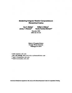
Figure 1: Current density decays of two cross-shaped structures after several hundred time steps, computed by LBMHD.

3.

LBMHD

Lattice Boltzmann methods (LBM) have proved a good alternative to conventional numerical approaches for simulating fluid flows and modeling physics in fluids [22]. The basic idea of the LBM is to develop a simplified kinetic model that incorporates the essential physics, and reproduces correct macroscopic averaged properties. Recently, several groups have applied the LBM to the problem of magneto-hydrodynamics (MHD) [9, 16] with promising results. LBMHD [17] simulates the behavior of a two-dimensional conducting fluid evolving from simple initial conditions and decaying to form current sheets. Figure 1 shows the current density decays of two cross-shaped structures after several hundred time steps as computed by LBMHD. The 2D spatial grid is coupled to an octagonal streaming lattice (shown in Figure 2a) and block distributed over a 2D processor grid. Each grid point is associated with a set of mesoscopic variables, whose values are stored in vectors proportional to the number of streaming directions – in this case nine (eight plus the null vector). The simulation proceeds by a sequence of collision and stream steps. A collision step involves data local only to that spatial point, allowing concurrent, dependence-free point updates; the mesoscopic variables at each point are updated through a complex algebraic expression originally derived from appropriate conservation laws. A stream step evolves the mesoscopic variables along the streaming lattice, necessitating communication between processors for grid points at the boundaries of the blocks. An example of a diagonal streaming vector updating three spatial cells is shown in Figure 2b. Additionally, an interpolation step is required between the spatial and stream lattices since they do not match. Overall the stream operation requires interprocessor communication, dense and strided memory copies, as well as third degree polynomial evaluations.

3.1

Porting details

Varying schemes were used in order to optimize the collision routine on each of the architectures. The basic computational structure consists of two nested loops over spatial grid points (typically 1001000 iterations) with inner loops over velocity streaming vectors and magnetic field streaming vectors (typically 10-30 iterations), performing various algebraic expressions. For the Power3/4 and Altix systems, the inner grid point loop was blocked to increase cache reuse – leading to a modest improvement in performance

Interprocessor communication was implemented using the MPI library, by copying the non-contiguous mesoscopic variables data into temporary buffers, thereby reducing the required number of send/receive messages. Additionally, a Co-array Fortran (CAF) [3] version was implemented for the X1 architecture. CAF is a onesided parallel programming language implemented via an extended Fortran 90 syntax. Unlike explicit message passing in MPI, CAF programs can directly access non-local data through co-array references. This allows a potential reduction in interprocessor overhead for architectures supporting one-sided communication, as well as opportunities for compiler-based optimizing transformations. For example, the X1’s measured latency decreased from 7.3 µsec using MPI to 3.9 µsec using CAF semantics [4]. In the CAF implementation of LBMHD, the spatial grid is declared as a co-array and boundary exchanges are performed using co-array subscript notation.

(a)

(b)

Figure 2: LBMHD’s (a) the octagonal streaming lattice coupled with the square spatial grid and (b) example of diagonal streaming vector updating three spatial cells.

3.2

Performance Results

Table 3 presents LBMHD performance on the five studied architecture for grid sizes of 40962 and 81922 . Note that to maximize performance the processor count is restricted to squared integers. The vector architectures show impressive results, achieving a speedup of approximately 44x, 16x, and 7x compared with the Power3, Power4, and Altix respectively (for 64 processors). The AVL and VOR are near maximum for both vector systems, indicating that this application is extremely well-suited for vector platforms. In fact the 3.3 Tflop/s attained on 1024 processor of the ES represents the highest performance of LBMHD on any measured architecture to date. The X1 gives comparable raw performance to the ES for most of our experiments; however for 256 processors on the large (81922 ) grid configuration, the ES ran about 1.5X faster due to the decreased scalability of the X1. Additionally, the ES consistently sustains a significantly higher fraction of peak, due in part to its superior CPU-memory balance. The X1 CAF implementation shows about a 10% overall improvement over the MPI version for

Grid Size

P

4096 x 4096

16 64 256 64 256 1024

8192 x 8192

Power3 Gflops/P %Pk 0.107 7% 0.142 9% 0.136 9% 0.105 7% 0.115 8% 0.108 7%

Power4 Gflops/P %Pk 0.279 5% 0.296 6% 0.281 5% 0.270 5% 0.278 5% — —

Altix Gflops/P 0.598 0.615 — 0.645 — —

%Pk 10% 10% — 11% — —

ES Gflops/P 4.62 4.29 3.21 4.64 4.26 3.30

%Pk 58% 54% 40% 58% 53% 41%

X1 (MPI) Gflops/P %Pk 4.32 34% 4.35 34% — — 4.48 35% 2.70 21% — —

X1 (CAF) Gflops/P %Pk 4.55 36% 4.26 33% — — 4.70 37% 2.91 23% — —

Table 3: LBMHD per processor performance on 4096x4096 and 8192x8192 grids.

the large test case, however MPI slightly outperformed CAF for the smaller grid size (P=64). For LBMHD, CAF reduced the memory traffic by a factor of 3X by eliminating user- and system-level message copies (latter used by MPI); these gains were somewhat offset by CAF’s use of more numerous and smaller sized messages. This issue will be the focus of future investigation. The low performance of the superscalar systems is mostly due to limited memory bandwidth. LBMHD has a low computational intensity – about 1.5 FP operations per data word of access – making it extremely difficult for the memory subsystem to keep up with the arithmetic units. Vector systems are able to address this discrepancy through a superior memory system and support for deeply pipelined memory fetches. Additionally, the 40962 and 81922 grids require 7.5 GB and 30 GB of memory respectively, causing the subdomain’s memory footprint to exceed the cache size even at high concurrencies. Nonetheless, the Altix outperforms the Power3 and Power4 in terms of Gflop/s and fraction of peak due to its higher memory bandwidth and superior network characteristics. Observe that superscalar performance relative to concurrency shows more complex behavior than on the vector systems. Since the cache-blocking algorithm for the collision step is not perfect, certain data distributions are superior to others – accounting for increased performance at intermediate concurrencies. At larger concurrencies, the cost of communication begins to dominate, thus reducing performance as in the case of the vector systems.

4.

PARATEC

PARATEC (PARAllel Total Energy Code [5]) performs ab-initio quantum-mechanical total energy calculations using pseudopotentials and a plane wave basis set. The pseudopotentials are of the standard norm-conserving variety. Forces can be easily calculated and used to relax the atoms into their equilibrium positions. PARATEC uses an all-band conjugate gradient (CG) approach to solve the Kohn-Sham equations of Density Functional Theory (DFT) and obtain the ground-state electron wavefunctions. DFT is the most commonly used technique in materials science, having a quantum mechanical treatment of the electrons, to calculate the structural and electronic properties of materials. Codes based on DFT are widely used to study properties such as strength, cohesion, growth, magnetic, optical, and transport for materials like nanostructures, complex surfaces, and doped semiconductors. Due to its accurate predictive power and computational efficiency, DFT based codes have been one of the largest consumer of supercomputing cycles in computer centers around the world. Figure 4 shows the induced current and charge density in crystalized glycine, calculated using PARATEC. These simulations are used to better understand nuclear magnetic resonance experiments [24].

Figure 3: Visualization of induced current (white arrows) and charge density (colored plane and grey surface) in crystalized glycine, described in [24].

4.1

Porting Details

In solving the Kohn-Sham equations using a plane wave basis, part of the calculation is carried out in real space and the remainder in Fourier space using specialized parallel 3D FFTs to transform the wavefunctions. The code typically spends most of its time in vendor supplied BLAS3 (˜30%) and 1D FFTs (˜30%) on which the 3D FFTs libraries are built, with the remaining time in handcoded F90. For this reason, PARATEC generally obtains a high percentage of peak performance across a spectrum of computing platforms. The code exploits fine-grained parallelism by dividing the plane wave (Fourier) components for each electron among the different processors [5]. PARATEC is written in F90 and MPI and is designed primarily for massively parallel computing platforms, but can also run on serial machines. The code has run on many computer architectures and uses preprocessing to include machine-specific routines such as the FFT calls. Previous work examined vectorized PARATEC performance on a single NEC SX-6 node [21], making porting to the ES and X1 a relatively simple task. Since much of the computation involves FFTs and BLAS3, an efficient vector implementation of these libraries is critical for high performance. However, while this was true for the BLAS3 routines on the ES and X1, the standard vendor supplied 1D FFT routines (on which our own specialized 3D FFTs are written) run at a relatively low percentage of peak. Code transformation was therefore required to rewrite our 3D FFT routines to use simultaneous (often called multiple) 1D FFT calls, which allow effective vectorization across many 1D FFTs. Additionally, compiler directives were in-

P 32 64 128 256 512 1024

Power3 Gflops/P %Pk 0.950 63% 0.848 57% 0.739 49% 0.572 38% 0.413 28% — —

Power4 Gflops/P %Pk 2.02 39% 1.73 33% 1.50 29% 1.08 21% — — — —

432 Atom Altix Gflops/P %Pk 3.71 62% 3.24 54% — — — — — — — —

686 Atom ES Gflops/P 4.76 4.67 4.74 4.17 3.39 2.08

%Pk 60% 58% 59% 52% 42% 26%

X1 Gflops/P 3.04 2.59 1.91 — — —

%Pk 24% 20% 15% — — —

ES Gflops/P — 5.25 4.95 4.59 3.76 2.53

%Pk — 66% 62% 57% 47% 32%

X1 Gflops/P — 3.73 3.01 1.27 — —

%Pk — 29% 24% 10% — —

Table 4: PARATEC per processor performance on a 432 and 686 atom Silicon Bulk system.

(a)

(b)

Figure 4: A three-processor example of PARATEC’s parallel data layout for the wavefunctions of each electron in (a) Fourier space and (b) real space.

serted to force the vectorization (and multistreaming on the X1) of loops that contain indirect addressing.

4.2

Performance Results

Table 4 presents performance data for 3 CG steps of a 432 and 686 Silicon atom bulk systems and a standard LDA run of PARATEC with a 25 Ry cut-off using norm-conserving pseudopotentials. A typical calculation would require between 20 and 60 CG iterations to converge the charge density. PARATEC runs at a high percentage of peak on both superscalar and vector-based architectures due to the heavy use of the computationally intensive FFTs and BLAS3 routines, which allow high cache reuse and efficient vector utilization. The main limitation to scaling PARATEC to large numbers of processors is the distributed grid transformation during the parallel 3D FFTs which requires global interprocessor communications. It was therefore necessary to write specialized 3D FFT to reduce these communication requirements. Since our 3D FFT routine maps the wavefunction of the electron from Fourier space, where it is represented by a sphere, to a 3D grid in real space – a significant reduction in global communication can be achieved by only transposing the non-zero grid elements. Nonetheless, architectures with a poor balance between their bisection bandwidth and computational rate (see Table 1) will suffer performance degradation at higher concurrencies due to global communication requirements. Figure 4 presents a visualization of the parallel data layout for the wavefunctions of each electron in Fourier space and real space. For the Fourier-space calculation, the wavefunction is represented by a sphere of points, divided by columns among the processors. Figure 4a shows a three-processor example (P 0, P 1, P 2), where each color represents the processor assignment of a given column. The

computation in Fourier space is load balanced by assigning each processor approximately the same number of points. The loadbalancing algorithm first orders the columns in descending order, and then distributes them among the processors such that the nextavailable column is assigned to the processor containing the fewest points. (The number of points a processor has corresponds to the total length of columns it holds.) The real-space data layout of the wavefunctions is on a standard Cartesian grid, where each processor holds a contiguous part of the space arranged in columns, as shown in Figure 4b. PARATEC uses a specialized 3D FFT to transform between these two data layouts with a minimum amount of interprocessor communication. The data is arranged in columns as the 3D FFT is performed, by taking 1D FFTs along the Z, Y, and X directions with parallel data transposes between each set of 1D FFTs. Results in Table 4 show that PARATEC achieves impressive performance on the ES, sustaining 2.6 Tflop/s for 1024 processors for the larger system – the first time that any architecture has attained over a Teraflop for this code. The declining performance at higher processor counts is caused by the increased communication overhead of the 3D FFTs, as well as reduced vector efficiency due to the decreasing vector length of this fixed-size problem. Since only 3 CG steps were performed in our benchmarking measurements, the set-up phase accounted for a growing fraction of the overall time – preventing us from accurately gathering the AVL and VOR values. The set-up time was therefore subtracted out for the reported Gflop/s measurements. This overhead becomes negligible for actual physical simulations, which require as many as 60 CG steps. For example on the smaller 432 atom system on 32 processors, the measured AVL for the total run was 145 and 46 for the ES and X1 (respectively); the AVL for only the CG steps (without set-up) would certainly be higher. Observe that X1 performance is lower than the ES, even though it has a higher peak speed. The code sections of handwritten F90, which typically consume about 30% of the run time, have a lower vector operation ratio than the BLAS3 and FFT routines. These handwritten segments also run slower on the X1 than the ES, since unvectorized code segments tend not to multistream across the X1’s SSPs. In addition, the X1 interconnect has a lower bisection bandwidth network than the ES (see Table 1), increasing the overhead for the FFT’s global transpositions at higher processor counts. Thus, even though the code portions utilizing BLAS3 libraries run faster on the X1, the ES achieves higher overall performance. In fact, due to the X1’s poor scalability above 128 processors, the ES shows more than a 3.5X runtime advantage when using 256 processors on the larger 686 atom simulation. PARATEC runs efficiently on the Power3, but sustained performance (percent of peak) on the

Figure 5: Visualization of the grazing collision of two black holes computed by the Cactus code. (Visualization by Werner Benger/AEI.)

tion into 3D spatial hypersurfaces that represent different slices of space along the time dimension. In this formalism, the equations are written as four constraint equations and 12 evolution equations. Additional stability is provided by the BSSN modifications to the standard ADM method [8]. The evolution equations can be solved using a number of different numerical approaches, including staggered leapfrog, McCormack, Lax-Wendroff, and iterative CrankNicholson schemes. A “lapse” function describes the time slicing between hypersurfaces for each step in the evolution. A “shift metric” is used to move the coordinate system at each step to avoid being drawn into a singularity. The four constraint equations are used to select different lapse functions and the related shift vectors. For parallel computation, the grid is block domain decomposed so that each processor has a section of the global grid. The standard MPI driver for Cactus solves the PDE on a local grid section and then updates the values at the ghost zones by exchanging data on the faces of its topological neighbors in the domain decomposition (shown in Figure 6 by the 2D schematic diagram).

Power4 is lower due, in part, to network contention for memory bandwidth [21]. The loss in scaling on the Power3 is primarily caused by the increased communication cost as concurrency grows to 512 processors. The Power4 system has a much lower bisectionbandwidth to processor speed ratio than the Power3 resulting in poorer scaling to large numbers of processors. The Altix performs well on this code (second only to the ES). This is due to the Itanium2’s high memory bandwidth, combined with interconnect network with reasonably-high bandwidth, and extremely low latency (see Table 1). However, higher scalability Altix measurements are not available.

5.

CACTUS

One of the most challenging problems in astrophysics is the numerical solution of Einstein’s equations following from the Theory of General Relativity (GR): a set of coupled nonlinear hyperbolic and elliptic equations containing thousands of terms when fully expanded. The Cactus Computational ToolKit [2, 8] is designed to evolve Einstein’s equations stably in 3D on supercomputers to simulate astrophysical phenomena with high gravitational fluxes – such as the collision of two black holes and the gravitational waves radiating from that event. While Cactus is a modular framework supporting a wide variety of multi-physics applications [11], this study focuses exclusively on the GR solver, which implements the Arnowitt-Deser-Misner (ADM) Baumgarte-Shapiro-Shibata-Nakamura (BSSN) [8] method for stable evolutions of black holes. Figure 5 presents a visualization of one of the first simulations of the grazing collision of two black holes computed by the Cactus code2 . The merging black holes are enveloped by their “apparent horizon”, which is colorized by its gaussian curvature. The concentric surfaces that surround the black holes are equipotential surfaces of the gravitational flux of the outgoing gravity wave generated by the collision. The Cactus General Relativity components solve Einstein’s equations as an initial value problem that evolves partial differential equations on a regular grid using the method of finite differences. The core of the General Relativity solver uses the ADM formalism, also known also as the 3+1 form. For the purpose of solving Einstein’s equations, the ADM solver decomposes the solu2

Visualization by Werner Benger (AEI/ZIB) using Amira [1]

Figure 6: Cactus solves PDEs on the local grid section and then updates ghost zone values on the the faces of its topological neighbors, as show by the 2D schematic diagram.

5.1

Porting Details

For the superscalar systems, the computations on the 3D grid are blocked in order to improve cache locality. Blocking is accomplished through the use of temporary ‘slice buffers’, which improve cache reuse while modestly increasing the computational overhead. On vector architectures these blocking optimizations were disabled, since they reduced the vector length and inhibited performance. The ES compiler misidentified some of the temporary variables in the most compute-intensive loop of the ADM-BSSN algorithm as having inter-loop dependencies. When attempts to force the loop to vectorize failed, a temporary array was created to break the phantom dependency. The cost of boundary condition enforcement is inconsequential on the microprocessor based systems, however they unexpectedly accounted for up to 20% of the ES runtime and over 30% of the X1 overhead. These costs were so extreme for some problems sizes on the X1 that a hard-coded implementation of vectorized boundary conditions was performed for the port. The

Grid Size

P

80x80x80 per processor

16 64 256 1024 16 64 256 1024

250x64x64 per processor

Power3 Gflops/P %Pk 0.314 21% 0.217 14% 0.216 14% 0.215 14% 0.097 6% 0.082 6% 0.071 5% 0.060 4%

Power4 Gflops/P %Pk 0.577 11% 0.496 10% 0.475 9% — — 0.556 11% — — — — — —

Altix Gflops/P 0.892 0.699 — — 0.514 0.422 — —

%Pk 15% 12% — — 9% 7% — —

ES Gflops/P 1.47 1.36 1.35 1.34 2.83 2.70 2.70 2.70

%Pk 18% 17% 17% 17% 35% 34% 34% 34%

X1 Gflops/P %Pk 0.540 4% 0.427 3% 0.409 3% — — 0.813 6% 0.717 6% 0.677 5% — —

Table 5: Cactus per processor performance on 80x80x80 and 250x64x64 grids

vectorized radiation boundaries reduced their runtime contribution from the most expensive part of the calculation to just under 5% of the overall wallclock time. The ES performance numbers presented here do not incorporate these additional boundary condition vectorizations due to our limited stay at the Earth Simulator Center, giving the X1 an advantage. Future ES experiments will incorporate these enhancements, thereby enabling a more direct comparison of the results.

5.2

Performance Results

The full-fledged production version of the Cactus ADM-BSSN application was run on the ES system with results for two grid sizes shown in Table 5. The problem size was scaled with the number of processors to keep the computational load the same (weak scaling). Cactus problems are typically scaled in this manner because their science requires the highest-possible resolutions. For the vector systems, Cactus achieves almost perfect VOR (over 99%) while the AVL is dependent on the x-dimension size of the local computational domain. Consequently, the larger problem size (250x64x64) executed with far higher efficiency on both vector machines than the smaller test case (AVL = 248 vs. 92), achieving 34% of peak on the ES. The oddly shaped domains for the larger test case were required because the ES does not have enough memory per node to support a 2503 domain. This rectangular grid configuration had no adverse effect on scaling efficiency despite the worse surface-to-volume ratio. Additional performance gains could be realized if the compiler was able to fuse the X and Y loop nests to form larger effective vector lengths. Recall that the boundary condition enforcement was not vectorized on the ES and accounts for up to 20% of the execution time, compared with less than 5% on the superscalar systems. This demonstrates a potential limitation of vector architectures: seemingly minor code portions that fail to vectorize can quickly dominate the overall execution time. The architectural imbalance between vector and scalar performance was particularly acute of the X1, which suffered a much greater impact from unvectorized code than the ES. As a result, significantly more effort went into code vectorization of the X1 port – without this optimization, the non-vectorized code portions would dominate the performance profile. Even with this additional vectorization effort, the X1 reached only 6% of peak. The majority of the wallclock time on the X1 went to the main GR solver subroutine (ADM BSSN Sources), which consumed 68% of the overall execution time. (The inner loops in ADM BSSN Sources were fully vectorized and the outer loops 100% multistreamed.) The next most expensive routine in the profile occupied only 4.5% of the execution time, leaving few opportunities for optimization in

the rest of the code. While the stand-alone extracted kernel of of the BSSN algorithm achieved an impressive 4.3Gflop/s on the X1, the maximum measured serial performance for the full-production version of Cactus was just over 1Gflop/s. Normally, the extracted kernel offers a good prediction of Cactus production performance, but the X1 presents us with a machine architecture that has confounded this prediction methodology. Cray engineers continue to investigate Cactus behavior on the X1. Table 5 shows that the ES reached an impressive 2.7 Tflop/s for the largest problem size using 1024 processors. This represents the highest per processor performance (by far) achieved by the full-production version of the Cactus ADM-BSSN on any evaluated system to date. The Power3, on the other hand, is 45 times slower than the ES, achieving only 60 Mflop/s per processor (6% of peak) at this scale for the larger problem size. The Power4 system offers even lower efficiency than the Power3 for the smaller (80x80x80) problem size, but still ranks high in terms of peak delivered performance in comparison to the X1 and Altix. We were unable to run the larger (250x64x64) problem sizes on the Power4 system, because there were insufficient high-memory nodes available to run these experiments. The Itanium2 processor on the Altix achieves good performance as a fraction of peak for smaller problem sizes (using the latest Intel 8.0 compilers). Observe that unlike vector architectures, microprocessor-based systems generally perform better on the smaller per-processor problem size because of better cache reuse. In terms of communication overhead, the ES spends 13% of the overall Cactus time in MPI compared with 23% on the Power3; highlighting the superior architectural balance of the network design for the ES. The Altix offered very low communication overhead, but its limited size prevented us from evaluating high-concurrency performance. The relatively low scalar performance on the microprocessor-based systems is partially due to register spilling, which is caused by the large number of variables in the main loop of the BSSN calculation. In addition, the IBM hardware prefetch engines appear to have difficulty with calculations involving multi-layer ghost zones on the boundaries. The unit-stride regularity of memory accesses (necessary to activate automatic prefetching) is broken as the calculation skips over the ghost zones at the boundaries, thereby keeping the hardware streams disengaged for the majority of the time [12]. As a result the processor ends up stalled on memory requests even though only a fraction of the available memory bandwidth is utilized. IBM is aware of this behavior and has added new variants of the prefetch instructions to the Power5 for keeping the prefetch streams engaged when exposed to minor data-access irregularities. We look forward to testing Cactus on the Power5 platform when it becomes available.

nels. This type of calculation helped to shed light on “anomalous” energy transport that was observed in real experiments.

6.1

Figure 7: 3D visualization of electrostatic potential in global, self-consistent GTC simulation of plasma microturbulence in a magnetic fusion device.

6.

Porting details

Although the PIC approach drastically reduces the computational requirements, the grid-based charge deposition phase is a source of performance degradation for both superscalar and vector architectures. Randomly localized particles deposit their charge on the grid, thereby causing poor cache reuse on superscalar machines. The effect of this deposition step is more pronounced on vector system, since two or more particle may contribute to the charge at the same grid point – creating a potential memory-dependency conflict. Figure 8 presents a visual representation of the PIC grid charge deposition phase. In the classic PIC method a particle is followed directly and its charge is distributed to its nearest neighboring grid points (see Figure 8a). However, in the GTC gyrokinetic PIC approach, the fast circular motion of the charged particle around the magnetic field lines is averaged out and replaced by a charged ring. The 4-point average method consists of picking four points on that charged ring, each one having a fraction of the total charge, and distributing that charge to the nearest grid points (see Figure 8b). In this way, the full influence of the fast, circular trajectory is preserved without having to resolve it. However, this methodology inhibits vectorization since multiple particles may concurrently attempt to deposit their change onto the same grid point.

GTC

The Gyrokinetic Toroidal Code (GTC) is a 3D particle-in-cell (PIC) application developed at the Princeton Plasma Physics Laboratory to study turbulent transport in magnetic confinement fusion [15, 14]. Turbulence is believed to be the main mechanism by which energy and particles are transported away from the hot plasma core in fusion experiments with magnetic toroidal devices. An in-depth understanding of this process is of utmost importance for the design of future experiments since their performance and operation costs are directly linked to energy losses. At present, GTC solves the non-linear gyrophase-averaged VlasovPoisson equations [13] for a system of charged particles in a selfconsistent, self-generated electrostatic field. The geometry of the system is that of a torus with an externally imposed equilibrium magnetic field, characteristic of toroidal fusion devices. By using the PIC method, the non-linear partial differential equation describing the motion of the particles in the system becomes a simple set of ordinary differential equations that can be easily solved in the Lagrangian coordinates. The self-consistent electrostatic field driving this motion could conceptually be calculated directly from the distance between each pair of particles using an N 2 calculation, but this method quickly becomes computationally prohibitive as the number of particles increases. The PIC approach reduces the computational complexity to N , by using a grid where each particle deposits its charge to a limited number of neighboring points according to its range of influence. The electrostatic potential is then solved everywhere on the grid using the Poisson equation, and forces are gathered back to each particle. The most computationally intensive parts of GTC are the charge deposition and gather-push steps. Both involve large loops over the number of particles, which can reach several million per domain partition. Figure 7 shows the 3D visualization of electrostatic potential in global, self-consistent GTC simulation of plasma microturbulence in a magnetic fusion device. The elongated “finger-like” structures are turbulent eddies that act as energy and particle transport chan-

(a)

(b)

Figure 8: Charge deposition in (a) the classic PIC method and (b) the 4-point averaging of GTC’s gyrokinetic PIC approach. Fortunately, several methods have been developed to address the charge-deposition memory-dependency issue during the past two decades. Our approach uses the work-vector algorithm [19], where a temporary copy of the grid array is given an extra dimension corresponding to the vector length. Each vector operation acts on a given data set in the register then writes to a different memory address, entirely avoiding memory dependencies. After the main loop, the results accumulated in the work-vector array are gathered to the final grid array. The only drawback of this method is the increased memory footprint, which can be 2 to 8 times higher than the nonvectorized code version. Other approaches address this memory dependency problem via particle sorting strategies which increase the computational overhead and overall time to solution. Since GTC has previously been vectorized on a single-node SX6 [21], porting to the ES was relatively straightforward. However, performance was initially limited due to memory bank conflicts, caused by an access concentration to a few small 1D arrays. Using the duplicate pragma directive alleviated this problem by allowing the compiler to create multiple copies of the data structures across

Part/ Cell

Code

10

MPI

100

MPI Hybrid

P 32 64 32 64 1024

Power3 Gflops/P %Pk 0.135 9% 0.132 9% 0.135 9% 0.133 9% 0.063 4%

Power4 Gflops/P %Pk 0.299 6% 0.324 6% 0.293 6% 0.294 6%

Altix Gflops/P 0.290 0.257 0.333 0.308

%Pk 5% 4% 6% 5%

ES Gflops/P 0.961 0.835 1.34 1.25

%Pk 12% 10% 17% 16%

X1 Gflops/P %Pk 1.00 8% 0.803 6% 1.50 12% 1.36 11%

Table 6: GTC per processor performance using 10 and 100 particles per cell.

numerous memory banks. This method significantly reduced the bank conflicts in the charge deposition routine and increased its performance by 37%. Additional optimizations were performed to other code segments with various performance improvements. GTC is parallelized at a coarse-grain level using message-passing constructs. Although the MPI implementation achieves almost linear scaling on most architectures, the grid decomposition is limited to approximately 64 subdomains. To run at higher concurrency, a second level of fine-grain loop-level parallelization is implemented using OpenMP directives. However, the increased memory footprint created by the work-vector method inhibited the use of looplevel parallelism on the ES. A possible solution could be to add another dimension of domain decomposition to the code. This would require extensive code modifications and will be examined in future work. Our short stay at the Earth Simulator Center prevented further optimization. Porting to the X1 was straightforward from the vectorized ES version but initial performance was limited. Note that the X1 suffers from the same memory increase as the ES due to the work-vector approach, potentially inhibiting OpenMP parallelism. Several additional directives were necessary to allow effective multistreaming within each MSP. After discovering that the FORTRAN intrinsic function modulo was preventing the vectorization of a key loop in the gather-push routine, it was replaced by an equivalent but vectorizable statement mod. The most time consuming routine on the X1 became the ’shift’ subroutine. This step verifies the coordinates of newly moved particles to determine whether they have crossed a subdomain boundary and therefore require processor migration. The shift routine contains nested if statements that prevent the compiler from successfully vectorizing that code region. However, the non-vectorized shift routine accounted for significantly more overhead on the X1 than the ES (54% vs. 11% of overall time). Although both architectures have the same relative vector to scalar peak performance (8/1), serialized loops incur an even larger penalty on the X1. This is because in a serialized segment of a multistreamed code, only one of the four SSP scalar processors within an MSP can do useful work, thus degrading the relative performance ratio to 32/1. Performance on the X1 was improved by converting the nested if statements in the shift routine into two successive condition blocks, allowing the compiler to stream and vectorize the code properly. The overhead therefore decreased from 54% to only 4% of the total time. This optimization has not been implemented on the ES.

6.2

Performance Results

Table 6 presents GTC performance results on the five architectures examined in our study. The first test case is configured for standard production runs using 10 particles per grid cell (2 million grid point, 20 million particles). The second experiment examines 100

particles per cell (200 million particles), a significantly higher resolution that improves the overall statistics of the simulation while significantly (8 fold) increasing the time-to-solution – making it prohibitively expensive on most superscalar platforms. For the large test case, both the ES and X1 attain high AVL (228 and 62 respectively) and VOR (99% and 97%), indicating that the application has been suitably vectorized; in fact, the vector results represent the highest GTC performance on any tested platform to date. In absolute terms the X1 shows the highest performance, achieving 1.50 Gflop/s on the largest problem size for P=32 (1.87 Gflop/s in usertime) – a 12% improvement over the ES; however, recall that the ES version does not incorporate the vectorized shift routine, giving the X1 an advantage. Nonetheless, the ES sustains 17% of peak compared with only 12% on the X1. It should also be noted that because GTC uses single precision arithmetic, the X1 theoretical peak performance is actually 25.6 Gflop/s; however limited memory bandwidth and code complexity that inhibits compiler optimizations obviate this extra capability. Comparing performance with the superscalar architectures, the vector processors are about 10X, 5X, and 4X faster than the Power3, Power4 and Altix systems (respectively). Observe that using 1024 processors of the Power3 (in hybrid MPI/OpenMP mode) is still about 20% slower than 64-way vector runs; GTC’s OpenMP parallelism is currently unavailable on the vector systems, limiting concurrency to 64 processors (see Section 6.1). Within the superscalar platforms, the Altix shows the highest raw performance at over 300 Mflop/s, while the Power3 sustains the highest fraction of peak (9% compared with approximately 6% on the Power4 and Altix). Examining scalability from 32 to 64 processor, the ES and X1 performance drop 9% (7%) and 20% (9%) respectively, using a fixed size problem of 10 (100) particles per cell. This is primarily due to shorter loop sizes and correspondingly smaller vector lengths, as well as increased communication overhead. Superscalar architectures, while also suffering from communication overhead, actually benefit from smaller subdomains due to increased cache reuse. Results show that the Power3/4 sees little overall degradation when scaling from 32 to 64 processor (less than 3%), while the Altix suffers as much as 11%. This discrepancy is currently under investigation.

7.

SUMMARY AND CONCLUSIONS

This work compares performance between the parallel vector architectures of the ES and X1, and three leading superscalar platforms, the Power3, Power4, and Altix. We examined four diverse scientific applications with the potential to utilize ultrascale computing systems. Since most modern scientific codes are designed for (super)scalar microprocessors, it was necessary to port these applications onto the vector platforms; however only minor code transformations were applied in an attempt to maximize VOR and

Name LBMHD PARATEC CACTUS GTC Average

Power3 30.6 8.2 45.0 9.4 23.3

ES speedup vs. Power4 Altix 15.3 7.2 3.9 1.4 5.1 6.4 4.3 4.1 7.1 4.8

X1 1.5 3.9 4.0 0.9 2.6

Table 7: Summary of applications performance, based on largest comparable processor count and problem size.

Sustained Performance 60%

Power3 Power4 Altix ES X1

50%

40%

30%

20% Percent of Peak

AVL, extensive code reengineering has not been performed. Table 7 summarize the raw application performance relative to the ES, while sustained performance for a fixed concurrency (P=64) is shown in Figure 9. Overall results show that the ES vector system achieved excellent performance on our application suite – the highest of any architecture tested to date – demonstrating the tremendous potential of modern parallel vector systems. The ES consistently sustained a significantly higher fraction of peak than the X1, due in part to superior scalar processor performance, memory bandwidth, and network bisection bandwidth relative to the peak vector flop rate. A number of performance bottlenecks exposed on the vector machines relate to the extreme sensitivity of these systems to small amounts of unvectorized code. This sheds light on a different dimension of architectural balance than simple bandwidth and latency comparisons. It is important to note that X1-specific code optimizations have not been performed at this time. This complex vector architecture contains both data caches and multi-streaming processing units, and the optimal programming methodology is yet to be established. Finally, preliminary Altix results show promising performance characteristics; however, we tested a relatively small Altix platform and it is unclear if its network performance advantages would remain for large system configurations. The regularly structured, grid-based LBMHD simulation was extremely amenable to vectorization, achieving an amazing speed up of over 44X compared to the Power3 using 64 processors; the advantage was reduced to 30X when concurrency increased to 1024. This decrease in relative performance gain often occurs when comparing cache-based scalar and vector systems for fixed sized problems. As computational domains shrink with increasing processor counts, scalar architectures benefit from the improved cachereuse while vector platforms suffer a reduction in efficiency due to shorter vector lengths. Additionally, LBMHD highlighted the potential benefits of CAF programming, which improved the X1 raw performance to slightly exceed that of the ES for the large test case. Future work will examine CAF performance in more detail. PARATEC, a computationally intensive code, is well suited for most architectures as it typically spends most of its time in vendor supplied BLAS3(˜30%) and FFT(˜30%) routines. This electronic structures code requires the transformation of wavefunctions between real and Fourier space via specialized 3D FFTs. However, global communication during the grid transformation can become a bottleneck at high concurrencies. Here the ES significantly outperformed the X1 platform due to its superior architectural balance of bisection bandwidth relative to computation rate, achieving a runtime advantage of almost 4X. The grid structured, computationally intensive Cactus code was also well-suited for vectorization achieving up to a 45X improve-

10%

0% LBMHD

PARATEC

CACTUS

GTC

Figure 9: Sustained performance using 64 processors on largest comparable problem size (P=16 is shown for Cactus on the Power4).

ment on the ES compared with the Power3. However, the boundary condition calculation was unvectorized and consumed a much higher fraction of the overall runtime compared with superscalar systems (where this routine was insignificant). This example demonstrates that for large-scale numerical simulations even a small nonvectorizable code segment can quickly dominate the execution time from the properties of Amdahl’s Law. This is especially important in the context of multistreaming on the X1 architecture. Although both the ES and X1 have the same relative vector to scalar peak performance (8/1), serialized loops incur an even larger penalty on the X1. This is because in a serialized segment of a multistreamed code, only one of the four SSP scalar processors within an MSP can do useful work, thus degrading the relative performance ratio to 32/1. Finally, vectorizing the particle-in-cell GTC code highlighted some of the difficulties in expressing irregularly structured algorithms as a data-parallel program. However, once the code successfully vectorized, the vector architectures once again showed impressive performance, achieving a 4X to 10X runtime improvement over the scalar architectures in our study. The vector systems therefore have the potential for significantly higher resolution calculations that would otherwise be prohibitively expensive in terms of time-to-solution on conventional microprocessors. Implementing the vectorized version for this unstructured code, however, required the addition of temporary arrays, which increased the memory footprint dramatically (between 2X and 8X). This inhibited the use of OpenMP loop-level parallelization, and limited concurrency to a coarse grained distribution of 64 processors. This issue will be address in future work. Nonetheless, the 64-way vector systems still performed up to 20% faster than 1024 Power3 processors. Future work will extend our study to include applications in the areas of climate, molecular dynamics, cosmology, and combustion. We are particularly interested in investigating the vector performance of adaptive mesh refinement (AMR) methods, as we believe they will become a key component of future high-fidelity multiscale physics simulations, across a broad spectrum of application domains.

Acknowledgments The authors would like to gratefully thank: the staff of the Earth Simulator Center, especially Dr. T. Sato, S. Kitawaki and Y. Tsuda, for their assistance during our visit; D. Parks and J. Snyder of NEC America for their help in porting applications to the ES. Special thanks to Thomas Radke, Tom Goodale, and Holger Berger for assistance with the vector Cactus ports. This research used resources of the National Energy Research Scientific Computing Center, which is supported by the Office of Science of the U.S. Department of Energy under Contract No. DE-AC03-76SF00098. This research used resources of the Center for Computational Sciences at Oak Ridge National Laboratory, which is supported by the Office of Science of the Department of Energy under Contract DE-AC05-00OR22725. All authors from LBNL were supported by the Office of Advanced Scientific Computing Research in the Department of Energy Office of Science under contract number DEAC03-76SF00098. Dr. Ethier was supported by the Department of Energy under contract number DE-AC020-76-CH03073.

8.

REFERENCES

[1] Amira - Advanced 3D Visualization and Volume Modeling. http://www.amiravis.com. [2] Cactus Code Server. http://www.cactuscode.org.

[14] Z. Lin, S. Ethier, T.S. Hahm, and W.M. Tang. Size scaling of turbulent transport in magnetically confined plasmas. Phys. Rev. Lett., 88, 2002. [15] Z. Lin, T. S. Hahm, W. W. Lee, W. M. Tang, and R. B. White. Turbulent transport reduction by zonal flows: Massively parallel simulations. Science, Sep 1998. [16] A. Macnab, G. Vahala, P. Pavlo, , L. Vahala, and M. Soe. Lattice boltzmann model for dissipative incompressible MHD. In Proc. 28th EPS Conference on Controlled Fusion and Plasma Physics, volume 25A, Funchal, Portugal, June 18-22, 2001. [17] A. Macnab, G. Vahala, L. Vahala, and P. Pavlo. Lattice boltzmann model for dissipative MHD. In Proc. 29th EPS Conference on Controlled Fusion and Plasma Physics, volume 26B, Montreux, Switzerland, June 17-21, 2002. [18] K. Nakajima. Three-level hybrid vs. flat mpi on the earth simulator: Parallel iterative solvers for finite-element method. In Proc. 6th IMACS Symposium Iterative Methods in Scientific Computing, volume 6, Denver, Colorado, March 27-30, 2003. [19] A. Nishiguchi, S. Orii, and T. Yabe. Vector calculation of particle code. J. Comput. Phys., 61, 1985.

[3] Co-Array Fortran. http://www.co-array.org. [4] ORNL Cray X1 Evaluation. http://www.csm.ornl.gov/˜dunigan/cray. [5] PARAllel Total Energy Code. http://www.nersc.gov/projects/paratec. [6] Top500 Supercomputer Sites. http://www.top500.org. [7] P. A. Agarwal et al. Cray X1 evaluation status report. In Proc. of the 46th Cray Users Group Conference, May 17-21, 2004. [8] M. Alcubierre, G. Allen, B. Brgmann, E. Seidel, and W.-M. Suen. Towards an understanding of the stability properties of the 3+1 evolution equations in general relativity. Phys. Rev. D, (gr-qc/9908079), 2000. [9] P.J. Dellar. Lattice kinetic schemes for magnetohydrodynamics. J. Comput. Phys., 79, 2002. [10] T. H. Dunigan Jr., M. R. Fahey, J. B. White III, and P. H. Worley. Early evaluation of the Cray X1. In Proc. SC2003: High performance computing, networking, and storage conference, Phoenix, AZ, Nov 15-21, 2003. [11] J. A. Font, M. Miller, W. M. Suen, and M. Tobias. Three dimensional numerical general relativistic hydrodynamics: Formulations, methods, and code tests. Phys. Rev. D, Phys.Rev. D61, 2000. [12] G. Griem, L. Oliker, J. Shalf, and K. Yelick. Identifying performance bottlenecks on modern microarchitectures using an adaptable probe. In Proc. 3rd International Workshop on Performance Modeling, Evaluation, and Optimization of Parallel and Distributed Systems (PMEO-PDS), Santa Fe, New Mexico, Apr. 26-30, 2004. [13] W. W. Lee. Gyrokinetic particle simulation model. J. Comp. Phys., 72, 1987.

[20] L. Oliker, R. Biswas, J. Borrill, A. Canning, J. Carter, J. Djomehri, H. Shan, and D. Skinner. A performance evaluation of the Cray X1 for scientific applications. In VECPAR: 6th International Meeting on High Performance Computing for Computational Science, Valencia, Spain, June 28-30, 2004. [21] L. Oliker, A. Canning, J. Carter, J. Shalf, D. Skinner, S. Ethier, R. Biswas, J. Djomehri, and R. Van der Wijngaart. Evaluation of cache-based superscalar and cacheless vector architectures for scientific computations. In Proc. SC2003: High performance computing, networking, and storage conference, Phoenix, AZ, Nov 15-21, 2003. [22] S. Succi. The lattice boltzmann equation for fluids and beyond. Oxford Science Publ., 2001. [23] H. Uehara, M. Tamura, and M. Yokokawa. MPI performance measurement on the Earth Simulator. Technical Report # 15, NEC Research and Development, 2003/1. [24] Y-G Yoon, B.G. Pfrommer, S.G. Louie, and A. Canning. NMR chemical shifts in amino acids: effects of environments, electric field and amine group rotation. Solid State Communications, 131, 2004.