SciQL, Bridging the Gap between Science and Relational DBMS Ying Zhang
Martin Kersten
Milena Ivanova
Niels Nes
Centrum Wiskunde & Informatica Amsterdam, The Netherlands
Ying.Zhang, Martin.Kersten, Milena.Ivanova,
[email protected] ABSTRACT Scientific discoveries increasingly rely on the ability to efficiently grind massive amounts of experimental data using database technologies. To bridge the gap between the needs of the Data-Intensive Research fields and the current DBMS technologies, we propose SciQL (pronounced as ‘cycle’), the first SQL-based query language for scientific applications with both tables and arrays as first class citizens. It provides a seamless symbiosis of array-, set- and sequenceinterpretations. A key innovation is the extension of value-based grouping of SQL:2003 with structural grouping, i.e., fixed-sized and unbounded groups based on explicit relationships between elements positions. This leads to a generalisation of window-based query processing with wide applicability in science domains. This paper describes the main language features of SciQL and illustrates it using time-series concepts.
Categories and Subject Descriptors E.1 [Data Structures]: Arrays; H.2.3 [Languages]: Query languages; H.2.8 [Database Applications]: Scientific databases
General Terms Language
Keywords SciQL, array query language, array database, scientific databases, time series
1.
INTRODUCTION
The array computational paradigm is prevalent in most sciences and it has drawn attention from the database research community for many years. The object-oriented database systems of the ’90s allowed any collection type to be used recursively [4] and multidimensional database systems took it as the starting point for their design [21]. The hooks provided in relational systems for user defined functions and data types create a stepping stone towards interaction with array-based libraries, i.e. RasDaMan [6] is one of the
Permission to make digital or hard copies of all or part of this work for personal or classroom use is granted without fee provided that copies are not made or distributed for profit or commercial advantage and that copies bear this notice and the full citation on the first page. To copy otherwise, to republish, to post on servers or to redistribute to lists, requires prior specific permission and/or a fee. IDEAS11 2011, September 21-23, Lisbon [Portugal] Editors: Bernardino, Cruz, Desai c 2011 ACM 978-1-4503-0627-0/11/09 ...$10.00. Copyright
few systems in this area that have matured beyond the laboratory stage. Nevertheless, the array paradigm taken in isolation is insufficient to create a full-fledged scientific information system. Such a system should blend measurements with static and derived metadata about the instruments and observations. It therefore calls for a strong symbiosis of the relational paradigm and array paradigm. The SciQL language presented in this paper fills this gap. The mismatch between application needs and database technology has a long history, e.g., [22, 8, 55, 20, 23, 21]. The main problems encountered with relational systems in science can be summed up as i) the impedance mismatch between query language and array manipulation, ii) the difficulty to write complex array-based expressions in SQL, iii) ARRAYs are not first class citizens, and iv) ingestion of terabytes of data is too slow. The traditional DBMS simply carries too much overhead. Moreover, much of the science processing involves use of standard libraries, e.g., LINPACK, and statistics tools, e.g., R. Their interaction with a database is often confined to a simplified data import/export facility. The proposed standard for management of external data (SQL3/MED) [42] has not materialised as a component in contemporary system offerings. A query language is needed that achieves a true symbiosis of the TABLE and ARRAY semantics in the context of existing external software libraries. This led to the design of SciQL, where arrays are made first class citizens by enhancing the SQL:2003 framework along three innovative lines: • Seamless integration of array-, set-, and sequence- semantics. • Named dimensions with constraints as a declarative means for indexed access to array cells. • Structural grouping to generalize the value-based grouping towards selective access to groups of cells based on positional relationships for aggregation. A TABLE and an ARRAY differ semantically in a straightforward manner. A TABLE denotes a (multi-) set of tuples, while an AR RAY denotes a (sparsely) indexed collection of tuples called cells. All cells covered by an array’s dimensions always exist conceptually and their non-dimensional attributes are initialised to a default value, while in a TABLE tuples only come into existence after an explicit insert operation. Arrays may appear wherever tables are allowed in an SQL expression, producing an array if the column list of a SELECT statement contains dimensional expressions. The SQL iterator semantics associated with TABLEs carry over to AR RAY s, but iteration is confined to cells whose non-dimensional attributes are not NULL. An important operation is to carve out an array slab for further processing. The windowing scheme in SQL:2003 is a step into this
y
null
y
null
y
null
null
0.0
3 null
null
null
0.0
3 0.0
0.0
0.0
0.0
null
null
2 null
null
0.0
null
2 0.0
0.0
0.0
0.0
1 0.0
0.0
0.0
0.0
1 0.0
0.0
0.0
0.0
1 null
0.0
null
null
1 0.0
0.0
0.0
0.0
0.0
0.0
0.0
null
null
null
null
null
null
0.0
0.0
0.0
1
2
3
1
2
3
1
2
3
1
2
3
0 0.0 0
null
0 null 0
x
(a) matrix
null
0 0.0 0
x
(b) stripes
null
null
0.0
null
null
0.0
2 null
null
3 0.0
0.0
0 0.0 0
x
(c) diagonal
null
null
0.0
0.0
null
0.0
0.0
null
0.0
2 0.0
null
null
y 3 0.0
x
(d) sparse
Figure 1: SciQL fixed arrays with different forms y
null
y
null
y
null
null
null
null 10.0
3 6.0
7.0
4.0
0.0
null
2 null
null 10.0 null
2 0.0
1.0
4.0
1.0
1 -1.0
0.0
3.0
4.0
1 1.0
2.0
3.0
4.0
1 2.0
6.0
0.0
5.0
0 0.0 0
1.0
2.0
3.0
null
null
null
3.0
8.0
2
3
1
2
3
0 9.0 0
0.0
1
0 null 0
1
2
3
null
(a) matrix
x
null
x
1 null 10.0 null
null
0 10.0 null null 1 2 0 null
null
(b) stripes
(c) diagonal
3
x
null
3 null
null
null
6.0
null
null
5.0
2 null
null
null
4.0
5.0
null
3 3.0
0.0
null
0.0
2 -2.0 -1.0
null
null
y
3 -3.0 -2.0 -1.0
x
(d) sparse
Figure 2: Results of updating the four fixed arrays by the first four queries in Section 2.2. direction. It was primarily introduced to better handle time series in business data warehouses and data mining. In SciQL, we take it a step further by providing an easy to use language feature to identify groups of cells based on their positional relationships. Each group forms a pattern, called a tile, which can be subsequently used to derive all possible incarnations for, e.g., statistical aggregation. One way to evaluate SciQL is to confront the language design with a functional benchmark. Unfortunately, the area of array- and time series databases is still too immature to expect a (commercially) endorsed and crystallised benchmark. Instead, we exercise the SciQL design using well-chosen use cases in various scientific domains. In our previous paper [33], we have shown the expressiveness of SciQL in Landsat and astronomy image processing. In this paper, we use SciQL on a different class of array problems, namely time series. Time series play a significant role in many science areas, such as statistics, econometrics, mathematical finance, (digital) signal processing and all kinds of sensor data. This paper is further organised as follows. Section 2 introduces SciQL through a series of examples. Section 3 demonstrates query functionality. Section 4 evaluates the language with a functional benchmark using seismological time series data. Section 5 discusses related work. Section 6 concludes the paper with a summary and an outlook on the open issues.
2.
LANGUAGE MODEL
In this section we summarize the features offered in SciQL concerning ARRAY definition, instantiation and modification, as well as coercions between TABLE and ARRAY.
2.1
Array Definitions
We purposely stay as close as possible to the syntax and semantics of SQL:2003. An ARRAY object definition reuses the syntax of TABLE with a few minor additions. An array has one-ormore dimensional attributes (for short: dimensions) and zero-ormore non-dimensional attributes. A dimension is a measurement of the size of the array in a particular named direction, e.g., “x”, “y”, “z” or “time”. A dimensional attribute is denoted by the keyword DIMENSION with optional constraints describing the dimension range. The data type of a dimension can be any of the basic scalar data types, including TIMESTAMP, FLOAT and VARCHAR. The non-dimensional attributes of an array can be of any data types a normal table column can be and they may use a DEFAULT clause to initialize their values. The default value may be arbitrarily taken from a scalar expression, a cell’s dimensional value(s) (i.e., the cell’s coordinates on the array dimensions) or a side-effect free function. Omission of the default or assignment of a NULL-value produces a ‘hole’, which is ignored by the built-in aggregation functions.
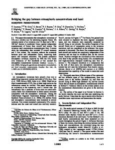
Arrays are either fixed or unbounded. An array is fixed iff all its dimensions are fixed, otherwise it is unbounded. The range and size of a fixed dimension are exactly specified using the sequence pattern [::], which is composed out of expressions each producing one scalar value. The interval between start and stop has an open end-point, i.e., stop is not included. For integer dimensions, the traditional syntax using an integer upper bound [] is allowed as a shortcut of the sequence pattern [0:1:]. Figure 1 shows four fixed arrays with different forms. In addition to the most common C-style rectangular arrays (Fig.1-a), stripes (Fig.1-b) can be defined as one where the default value of some rows is indistinguishable from out of bound access, i.e., those cells are explicitly excluded by carrying NULL values in their non-dimensional attributes. A diagonal array (Fig.1-c) is easily formulated using a predicate over the dimensions involved. It is even possible to carve out an array based on its content (Fig.1-d), thereby effectively nullifying all cells outside the domain of validity and producing a sparse array. This feature is of particular interest to remove outliers using an integrity constraint. Evidently, different array forms can lead to very different considerations with respect to their physical representation, a topic discussed in a companion paper. The following statements show how the four arrays in Figure 1 are created in SciQL: CREATE ARRAY matrix ( x INT DIMENSION[4], y INT DIMENSION[4], v FLOAT DEFAULT 0.0 ); CREATE ARRAY stripes ( x INT DIMENSION[4], y INT DIMENSION[4] CHECK(MOD(y,2) = 1), v FLOAT DEFAULT 0.0 ); CREATE ARRAY diagonal ( x INT DIMENSION[4], y INT DIMENSION[4] CHECK(x = y), v FLOAT DEFAULT 0.0 ); CREATE ARRAY sparse ( x INT DIMENSION[4], y INT DIMENSION[4], v FLOAT DEFAULT 0.0 CHECK(v BETWEEN 0 AND 10) );
A dimension is unbounded if any of its start, step, or stop expressions is identified by the pseudo expression *. A DIMEN SION clause without a sequence pattern implies the most open pattern [*:*:*]. Cells in an unbounded array can be modified using the INSERT and DELETE statements carried over from the table semantics. An unbounded array has an implicitly defined actual size derived from the minimal bounding rectangle that encloses all cells with an explicitly inserted non-NULL value in the array. When walking through an array instance, cells outside the minimal bounding rectangle are ignored. However, direct access to any cells within the array’s dimension bounds is guaranteed to produce the default value. The effect is that listing an array with unbounded dimensions still produces a finite result, but it may be huge. An unbounded dimension is typically used for an n-dimensional spatial array where only part of the dimension range designates a nonempty array cell. Time series are also prototypical examples of arrays with unbounded dimensions.
2.2
Array Modifications
The SQL update semantics is extended towards arrays in a straightforward manner. The array cells are initialised upon creation with
the default values. A cell is given a new value through an ordinary SQL UPDATE statement. A dimension can be used as a bound variable, which takes on all its dimension values (i.e., valid values of this dimension) successively. A convenient shortcut is to combine multiple updates into a single guarded statement. The evaluation order ensures that the first predicate that holds dictates the cell values. The refinement of the array matrix is shown in the first query below. The cells receive a zero only in the case x = y. The remaining queries demonstrate setting cell values in the arrays stripes, diagonal and sparse, respectively. The results are shown in Figure 2. UPDATE matrix SET v = CASE WHEN x > y THEN x + y WHEN x < y THEN x - y ELSE 0 END;
set to a non-NULL default. A selection excluding the user specified default values may solve this problem. An arbitrary table can be coerced into an array if the column list of the SELECT statement contains the dimension qualifiers ‘[’ and ‘]’ around a projection column, i.e., []. Here, the is a or a value expression. For instance, let mtable be the table produced by casting the array matrix to a table. It can be turned into an array by picking the columns forming the primary key in the column list as follows: SELECT [x], [y], v FROM mtable, or using the reverse cast operation CAST(mtable AS ARRAY(x,y)). The result is an unbounded array with actual size derived from the dimension column expressions [x] and [y]. The default values of all non-dimensional attributes are inherited from the default values in the original table.
UPDATE stripes SET v = x + y;
3.
UPDATE diagonal SET v = v + 10; UPDATE sparse SET v = MOD(RAND(),16);
null
null
Assignment of a NULL value to an array cell leads to a ‘hole’ in the array, a place indistinguishable from the out of bounds area. Such assignments overrule any predefined DEFAULT clause attached to the array definition. For convenience, the built-in array aggregate operations SUM (), COUNT (), AVG (), MIN () and MAX () are applied to non-NULL values only. y null Arrays can also be updated us3 -3.0 -2.0 0.0 0.0 ing INSERT and DELETE statements. Since all cells seman2 -2.0 -1.0 5.0 0.0 tically exists by definition, both 1 -1.0 0.0 4.0 0.0 operations effectively turn into 0 0.0 1.0 3.0 0.0 x update statements. The DELETE 1 2 3 0 null statement creates holes by assignFigure 3: Result of shifting a NULL value for all qualified ing and zero filling the cells. The INSERT statement simlast column of matrix. ply overwrites the cells at positions as specified by the input columns with new values. Note that although the UPDATE, INSERT and DELETE statements do not change the existence of array cells, for unbounded arrays they may result in scaling the minimal bounding rectangle up/down. The three queries below together illustrate how to delete a column in the array matrix where x = 2, then shift the remaining columns, and (manually) set the last column of matrix to its default value. In the second and third queries, the x and y dimensions of the array matrix are matched against the projection columns of the SELECT statements. Cells at matching positions are assigned new values (see Figure 3). DELETE FROM matrix WHERE x = 2; INSERT INTO matrix SELECT x-1, y, v FROM matrix WHERE x > 2; INSERT INTO matrix SELECT x, y, 0 FROM matrix WHERE x = 3;
2.3
Array and Table Coercions
One of the strong features of SciQL is to switch easily between a TABLE and an ARRAY perspective. Any array is turned into a corresponding table by simply selecting its attributes. The dimensions then form a compound primary key. For example, the matrix defined earlier becomes a table using the expression SELECT x, y, v FROM matrix or using a CAST operation like CAST(matrix AS TABLE). Note, that the semantics of an array leads to materialisation of all cells within the dimension bounds (or the minimal bounding rectangle for unbounded arrays), even if their values were
QUERY MODEL
From a query’s perspective, querying a TABLE and an ARRAY are much alike. In both cases elements are selected based on predicates, joins, and groupings. The result of any query expression is a table unless the column list contains the dimension qualifiers (‘[’ and ‘]’). A novel way to use GROUP BY, called tiling, is introduced to improve structure based querying.
3.1
Cell Selections
SELECT x, y, v FROM matrix WHERE v >2; SELECT [x], [y], v FROM matrix WHERE v >2; SELECT [T.k], [y], v FROM matrix JOIN T ON matrix.x = T.i;
The examples above illustrate a few simple array queries. The first query extracts values from the array matrix into a table. The second one constructs a sparse array from the selection, whose dimensional properties are inherited from the result set. The dimension qualifiers introduce a new dimension range, i.e., a minimal bounding box is derived from the result set, such that the answers fall within its bounds. The last query shows how elements of interest can be obtained from both arrays and tables using an ordinary join expression. It assumes a table T with two (or more) columns, where the column i is of a numeric type and the column k may be of any scalar type. The expression extracts the subarray from matrix and sets the bounds to the smallest enclosing bounding box defined by the values of the columns T.k and y. The actual bounds of an array can always be obtained from the built-in functions MIN () and MAX () over the dimensions.
3.2
Array Slicing
An ARRAY object can be considered an array of records in programming language terms. Therefore, the language supports positional index access conforming to the order the dimensions are introduced in the array definition. All attributes (dimensional and non-dimensional) of interest should be explicitly identified. A range pattern, borrowed from the programming language arena, supports easy slicing over individual dimensions using the aforementioned sequence pattern [::]. The range pattern is allowed in both the FROM and GROUP BY clauses. To illustrate this, we show a few slicing expressions over the arrays defined earlier (results are computed based on Fig. 2-a). SELECT * FROM matrix[3][2]; -- yields: (3, 2, 5.0) SELECT v FROM matrix[*][1:3]; -- yields: (-1.0), (-2.0), (0.0), (-1.0), (3.0), (0.0),(4.0),(5.0)
y
null
null
null
1 0.2 0.6 0.7 0.5
1 0.2 0.6 0.7 0.5
y
0 0.9 0.2 0.3 0.8 x 1 2 3 0 null
0 0.9 0.2 0.3 0.8 x 1 2 3 0 null
0 0.9 0.2 0.3 0.8 x 1 2 3 0 null
(a)
(b)
(c)
Anchor point
Anchor point
null
Anchor point
3 0.6 0.7 0.4 0.2 2 0.3 0.1 0.4 0.1
null
1 0.2 0.6 0.7 0.5
null
Anchor0.4 point0.1 2 0.3 0.1
null
3 0.6 0.7 0.4 0.2
2 0.3 0.1 0.4 0.1
null
3 0.6 0.7 0.4 0.2
2 0.3 0.1 0.4 0.1
null
y
null
3 0.6 0.7 0.4 0.2 null
1 0.2 0.6 0.7 0.5
0 0.9 0.2 0.3 0.8 x 1 2 3 0 null
(d)
Figure 4: SciQL Array Tiling y
null
y
null
y
null
null
null
3
0.450 0.425 0.400 0.275
3
null
0.425
null
0.275
null
2
0.250 0.300 0.450 0.425
2
null
null
null
1
0.300 0.450 0.425 0.300
1
null
null
null
null
1
0.550 0.475 0.450 0.575
1
0.360
null
null
0
0.475 0.450 0.575 0.650
0
0.475
null
0.575
null
0
0.900 0.550 0.250 0.550
0
1
2
3
1
2
3
0
1
null
(a)
2
3
x
null
x
0
(b)
1
null
2
3
x
null
null
null
null
null
0.425
null
null
2
0
(c)
0
null
null
3
0.425 0.400 0.275 0.150
null
0.650 0.550 0.300 0.200
2
null
null
y 3
null
The SQL UPDATE statement is extended to take array expressions directly. This leads to a more convenient and compact notation in many situations. The bounds of the subarray are specified by a sequence pattern of literals. Again, a sequence of updates act as a guarded function. The array dimensions are used as bound variables that run over all valid dimension values. This is illustrated using the queries below:
null
y
SELECT v FROM matrix[0:2:4][0:2:4]; -- yields: (0.0), (-2.0), (2.0), (0.0)
x
(d)
Figure 5: Results of computing AVG () over the tiles. UPDATE matrix SET matrix[0:2][*].v = v * 1.19; UPDATE matrix SET matrix[x][*].v = CASE WHEN v < 0 THEN x WHEN v >10 THEN 10 * x ELSE 0 END;
3.3
Array Views
A common case is to embed an array into a larger one, such that a zero initialised bounding border is created, or to shift a vector before moving averages are calculated. To avoid possible significant data movements, the array VIEW constructor can be used instead. The first two queries below illustrate an embedding, i.e., to transpose and shift an array, respectively. In the SELECT clause, the x and y columns are used to identify the cells in the vmatrix to be updated. The last example illustrates how the aforementioned example of shift with zero fill of a column (see Section 2.2, second query group) can be modelled as a view. Note that the results of all SELECT statements in the examples below are tables, thus in the third query, the ordinary SQL UNION semantics applies. CREATE VIEW ARRAY vmatrix ( x INT DIMENSION[-1:1:5], y INT DIMENSION[-1:1:5], w FLOAT DEFAULT 0.0 ) AS SELECT y, x, v FROM matrix;
to the anchor point. The value derived from a group aggregation is associated with the dimensional value(s) of the anchor point. Consider a 4 × 4 matrix and tiling it with a 2 × 2 matrix by extending the anchor point matrix[x][y] with structure elements matrix[x+1][y], matrix[x][y+1], and matrix[x+1][y+1]. The tiling operation performs a grouping for every valid anchor point on the actual array dimensions. Figure 4-a shows the first four tiles created. The individual elements of a group need not belong to the domain of the array dimensions, but then their values are assumed to be the outer NULL value, which are ignored in the statistical aggregate operations. This way we break the matrix array into 16 overlapping tiles. The number can be reduced by explicitly calling for DISTINCT tiles. This leads to considering each cell for one tile only, leaving a hole behind for the next candidate tile. Furthermore, in this case all tiles with holes do not participate in the result set. This means that for irregularly formed tiles there is no guarantee that all array cells are taking part in the grouping. The dimension range sequence pattern can be used to concisely define all values of interest. The following queries create the tiles on matrix as depicted in Figure 4 (in the order from left to right). The query results are shown in Figure 5.
CREATE VIEW ARRAY vector ( x INT DIMENSION[-1:1:5], w FLOAT DEFAULT 0.0 ) AS SELECT A.x, (A.v+B.v)/2 FROM matrix AS A JOIN (SELECT x+1 AS x, v FROM matrix) AS B ON A.x = B.x;
SELECT [x], [y], AVG(v) FROM matrix GROUP BY matrix[x:x+2][y:y+2];
CREATE VIEW ARRAY vmatrix2 ( x INT DIMENSION[-1:1:5], y INT DIMENSION[-1:1:5], w FLOAT DEFAULT 0.0 ) AS SELECT x, y, v FROM matrix WHERE x < 2 UNION SELECT x-1, y, v FROM matrix WHERE x > 2 UNION SELECT x, y, 0.0 FROM matrix WHERE x = 3;
SELECT [x], [y], AVG(v) FROM matrix GROUP BY matrix[x-1:x+1][y-1:y+1];
3.4
Aggregate Tiling
A key operation in science applications is to perform statistics on groups. They are commonly identified by an attribute or expression list in a GROUP BY clause. This value-based grouping can be extended to structural grouping for ARRAYs in a natural way. Large arrays are often broken into smaller pieces before being aggregated or overlaid with a structure to calculate, e.g., a Gaussian kernel function. SciQL supports fine-grained control over breaking an array into possibly overlapping tiles using a slight variation of the SQL GROUP BY clause semantics. Therefore, the attribute list is replaced by a parametrised series of array elements, called tiles. Tiling starts with an anchor point identified by its dimensional value(s), which is extended with a list of cell denotations relative
SELECT [x], [y], AVG(v) FROM matrix GROUP BY DISTINCT matrix[x:x+2][y:y+2];
SELECT [x], [y], AVG(v) FROM matrix[1:*][1:*] GROUP BY DISTINCT matrix[x][y], matrix[x-1][y], matrix[x+1][y], matrix[x][y-1], matrix[x][y+1];
A recurring operation is to derive check sums over array slabs. In SciQL this can be achieved with a simple tiling on, e.g., the x dimension. In this case, the anchor point is the value of x. For example: SELECT [x], SUM(v) FROM matrix GROUP BY matrix[x][*];
A discrete convolution operation is only slightly more complex. For, consider each element to be replaced by the average of its neighboring elements. The extended matrix vmatrix is used to calculate the convolution, because it ensures a zero value for all boundary elements. The aggregates outside the bounds [0:4][0:4] are not calculated by using an array slicing in the FROM clause.
SELECT [x], [y], AVG(v) FROM vmatrix[0:4][0:4] GROUP BY vmatrix[x-1:1:x+2][y-1:1:y+2];
Value based selection and structure based selection can be combined. An example is the nearest neighbor search, where the structure dictates the context over which a metric function is evaluated. Most systems dealing with feature vectors deploy a default metric, e.g., the Euclidean distance. The example below assumes such a distance function that takes an argument ?V as the reference vector. It generates a listing of all columns with the distance from the reference vector. Ranking the result produces the K-nearest neighbors. SELECT x, distance(matrix, ?V ) AS dist FROM matrix GROUP BY matrix[x][*] ORDER BY dist LIMIT 10;
Using the dimension values in the grouping clause permits complex structures to be defined. It generalises the SQL:2003 windowing functions, which are limited to aggregations over sliding windows with static bounds and shift count over a sequence. The SciQL approach can be generalised to support the equivalent of mask-based tile selections. For this we simply need a table with dimension values, which are used within the GROUP BY clause as a pattern to search for.
4.
TIME SERIES DATA PROCESSING
After introducing the main features of SciQL, we continue with illustrating its expressiveness as a time series language. Generally speaking, a time series is a sequence of data points with each point attached a time stamp. A time series can be regular or irregular. The data points in a regular time series are measured at successive times spaced at uniform time intervals. In the sciences, sensor data (e.g., temperature, ground motion and strain gauges) is often a regular time series, as it comes in as a continuous stream at a fixed rate. An irregular time series contains data points at successive times spaced at arbitrary time intervals. Sensor data with gaps is an irregular time series, in which the gaps typically indicate malfunctioning sensors. In the time series domain there does not exist a standardised functional test of expressiveness. Since the primary target of SciQL is the scientific domains, we take the data from seismology (an important scientific domain with a huge amount of time series data) as a yardstick. In this section, we first discuss how time series are supported by SciQL. Then we demonstrate how the typical operations of seismic signal processing can be easily and concisely phrased in SciQL.
4.1 4.1.1
Time Series Fixed Time Series
If experiments are conducted at regular intervals, it is helpful to represent them as arrays indexed by the time stamps with a fixed stride. The SciQL language constructs allow for easy subsequent manipulations, such as interpolation and computing moving averages, without the need to resort to self-joins. The following query shows how SciQL is turned into a time series supporting language by simply choosing a temporal domain for at least one dimension: CREATE ARRAY ts1 ( time TIMESTAMP DIMENSION[TIMESTAMP ‘2011-01-01 09:00:00’ : INTERVAL ‘1’ MINUTE : TIMESTAMP ‘2011-01-01 10:00:00’], data FLOAT DEFAULT 0.0 );
The data type of the time dimension is a TIMESTAMP and its increment is a temporal interval unit, e.g., a minute. This example creates a fixed time series array. The two statements in the following example are semantically identical, namely, they all populate the array with five values starting from the first cell with a step size of 2, overwriting the default values of these cells. Note, that they explicitly identify the cells whose values should be overwritten. INSERT INTO ts1 VALUES (‘2011-01-01 09:00’, 0.7793), (‘2011-01-01 09:02’, 0.9076), (‘2011-01-01 09:04’, 0.2267), (‘2011-01-01 09:06’, 0.2094), (‘2011-01-01 09:08’, 0.1295); UPDATE ts1 SET ts1[‘2011-01-01 09:00’: INTERVAL ‘2’ MINUTE : ‘2011-01-01 09:10’].data = (0.7793), (0.9076), (0.2267), (0.2094), (0.1295);
Insertions with explicit time values may contradict the definition of the time dimension. If the value is before start or after stop, the insertion is ignored. If the value is inside of the [start, stop) interval, but does not match any of the values defined by the temporal unit step, we apply gridding. That is, the data value will be inserted into a cell which dimensional values are the closest to the original timestamp. In the following query, the value of 47.00008 seconds will be rounded to 1 minute, so that the value 0.9216 is inserted into the cell with dimensional value of ‘2011-0101 09:01’: INSERT INTO ts1 VALUES (‘2011-01-01 09:00:47.00008’, 0.9216);
4.1.2
Unbounded Time Series
In many cases not all constraints of a time dimension are known in advance. For instance, a time series of the waveforms produced by a seismic sensor may only have a start time stamp but no stop time stamp, because once the measurement has started, it continues as long as possible. Moreover, sensor data often contains time gaps even if the sample rate is known beforehand, so it might not be desirable to enforce a step size in such time series, which can cause losing information about the gaps. This is where time series with unbounded (time) dimensions come in handy. The examples below show several variants of the ts1 defined above with some or all of the constraints start, step or stop omitted. The arrays ts3, ts4, and ts5 do not carry a step size, which means that any event time stamp up to a microsecond difference would be acceptable (microsecond is the smallest unit for a time stamp in SQL:2003). The dimensions here merely enforce an event order. CREATE ARRAY ts2 ( time TIMESTAMP DIMENSION[TIMESTAMP ‘2011-01-01 09:00:00’ : INTERVAL ‘1’ MINUTE : *], data FLOAT DEFAULT 0.0 ); CREATE ARRAY ts3 ( time TIMESTAMP DIMENSION[TIMESTAMP ‘2011-01-01 09:00:00’ : * : TIMESTAMP ‘2011-01-01 10:00:00’], data FLOAT DEFAULT 0.0 ); CREATE ARRAY ts4 ( time TIMESTAMP DIMENSION[TIMESTAMP ‘2011-01-01 10:00:00’: * : *], data FLOAT DEFAULT 0.0 ); CREATE ARRAY ts5 ( time TIMESTAMP DIMENSION, data FLOAT DEFAULT 0.0 );
Compared with fixed time series, inserting values into an unbounded time series without explicitly specifying the cell indices has several semantic differences. Basically, the values can be inserted at any positions satisfying the partial constraints of the time dimension in the array definition, as long as the relative order among the values is preserved. However, this operation can be made more deterministic by using the available constraints. Unbounded time series can be divided into the following classes, based on the absent dimension constraint(s): i) one end of the dimension range (i.e., start or stop); ii) both ends of the dimension range; iii) the step size; iv) one end of the dimension range and the step size; and v) all constraints. The first class is easy to handle. Consider the query: INSERT INTO ts2 VALUES (0.7793), (0.9076), (0.2267), (0.2094), (0.1295);
Since the array ts2 has a start and step for its time dimension, the values are inserted into the first five cells of the array (if the start was omitted, the last five cells are chosen), i.e., at the timestamps ‘2011-01-01 09:00’, ‘2011-01-01 09:01’, . . . , ‘201101-01 09:04’, overwriting any existing values at these positions. If both ends of the dimension ranges are omitted (class ii)), we take the current time now(), rounded to the granularity of the step size, as the starting position for insertions. When the step size is omitted (class iii)), we use the smallest unit of the dimension data type as the default step size. In case of timestamp, it is the microsecond. Thus, the query: INSERT INTO ts3 VALUES (0.7793), (0.9076), (0.2267), (0.2094), (0.1295);
produces the time series ((‘2011-01-01 09:00:00.000000’, 0.7793), . . . , (‘2011-01-01 09:00:00.000004’, 0.1295)). To handle the unbounded time series of the classes iv) and v), we combine the rules used for the first three classes. For instance, to handle the query: INSERT INTO ts5 VALUES (0.7793), (0.9076), (0.2267), (0.2094), (0.1295);
we take the value of now() as the start position and microsecond as the step size.
4.1.3
Interpolation
Applications often assume values at regular time intervals, while the available measurement time series may have gaps of missing values or values taken at irregular time intervals. In such cases interpolation can be used to provide approximate values at regular time steps. Consider the irregular time series ts4 set by the following query: INSERT INTO ts4 VALUES (‘2011-01-01 09:00’, 0.28), (‘2011-01-01 09:02’, 0.36), (‘2011-01-01 09:05’, 0.52);
The interpolation can be formulated in SciQL as follows. First, we create a fixed time series with the desired regular step, for instance 1 minute: CREATE ARRAY heartbeat ( time TIMESTAMP DIMENSION[TIMESTAMP ‘2011-01-01 09:00’ : INTERVAL ‘1’ MINUTE : TIMESTAMP ‘2011-01-01 10:00’], data FLOAT DEFAULT NULL );
The next step is to compute and insert the interpolated values at the regular time steps. To make the discussion concrete, we will use linear interpolation to compute the approximate data values: INSERT INTO heartbeat SELECT hb.time, irr.data + (hb.time - irr.time) * (irr[NEXT(irr, irr.time)].data - irr.data) / (NEXT(irr, irr.time) - irr.time) FROM heartbeat AS hb, ts4 AS irr WHERE hb.time >= irr.time AND hb.time ?delta;
Unfortunately, the events detected by this simple STA/LTA algorithm contain many events not associated to an earthquake (they could have been caused by a cow passing by). The false positives have to be filtered out. This can be done by checking events detected by neighbouring stations (see table Neighbours below), because a real seismic event should be detected by multiple stations with time delays within some known ranges (i.e., between mindelay and maxdelay) and some strength reduction of the seismic wave (i.e., weight).
-- detect isolated errors by direct environment -using wave propagation statics CREATE TABLE Neighbours ( sta1 VARCHAR(5), sta2 VARCHAR(5), mindelay INTERVAL SECOND, maxdelay INTERVAL SECOND, weight FLOAT ); -- detect false positives: DELETE FROM Event WHERE id NOT IN ( SELECT A.id FROM Event AS A, Event AS B, Neighbours AS N WHERE A.station = N.sta1 AND B.station = N.sta2 AND B.time BETWEEN A.time + N.mindelay AND A.time + N.maxdelay AND A.ratio > B.ratio * N.weight);
After having removed the false positives detected above from the Event table, smaller time series are retrieved from the original array and passed to some (external) UDFs for further analysis: SELECT myfunction(A[station].*) FROM MSeed AS A, Event AS B WHERE A.station = B.station AND A.time = B.time GROUP BY DISTINCT A[station][time - INTERVAL ‘1’ MINUTE : time + INTERVAL ‘2’ MINUTE];
4.2.2
Digital Signal Processing
Cross-correlation, convolution and Fourier transformation are fundamental operations in (seismological) Digital Signal Processing (DSP) [54]. They are provided as standard functions in many mathematical libraries, such as Matlab, Octave and Sage. Those functions can be easily hooked up in SciQL as external UDFs. However, to better utilise the query processing and optimisation facilities of DBMSs, one should be able to directly phrase these operations in queries. In SciQL this is easy, as all necessary features are present. Cross-correlation is one of the most commonly used operations in seismology, much like the join operations in database systems. In DSP, cross-correlation measures the similarity of two waveforms as a function of a time-lag applied to one of them. For two finite sequences f and g of real numbers, their cross-correlation is defined as: de f
( f ? g)[n] =
∞
∑
f [n]g[n + m]
m=−∞
To compute f ? g, one maps the sequences onto a two-dimensional plane with x- and y- axes, with g being fixed on the plane. Then, the sequence f is slided along the x axes from −∞ to ∞. Wherever the two sequences intersect, compute the product of all intersecting value pairs and sum all products up. Figure 6 shows an example of computing the cross-correlation of two sequences containing respectively 4 and 3 items. In SciQL, f ? g can be expressed as shown below. The query assumes two one-dimensional arrays F and G (e.g., time series around the events detected previously), each with an integer dimension pos (since the time stamps do not play a role in cross-correlation) and one FLOAT non-dimensional attribute val. The results of cross-correlating F and G are stored in the array CrCorr, which has an integer dimension with the values of n. For
each cell of CrCorr, the query takes the intersecting slices of F and G (in the GROUP BY clause) to compute the products and sum. The built-in functions MIN() and MAX() return the smaller/larger value of its two parameters, which are used to prevent array slicing from going out of the dimension bounds. DECLARE fmin INT, SET fmin = SELECT SET fmax = SELECT SET fcnt = SELECT SET gmin = SELECT SET gcnt = SELECT SET n = -fmax;
fmax INT, fcnt INT, gmin INT, gcnt INT, n INT; MIN(pos) FROM F; MAX(pos) FROM F; COUNT(*) FROM F; MIN(pos) FROM G; COUNT(*) FROM G;
CREATE ARRAY CrCorr ( idx INT DIMENSION[n:1:gcnt], val FLOAT DEFAULT 0.0 ); INSERT INTO CrCorr SELECT C.idx, SUM(F.val * G.val) FROM F, G, CrCorr AS C GROUP BY F[MAX(fmin, -C.idx) : MIN(fcnt, gcnt-C.idx)], G[MAX(gmin, C.idx) : MIN(gcnt, fcnt+C.idx)];
Computing the convolution of two sequences f ∗ g is another important operation in seismology. It is used in, e.g., design and implementation of Finite Impulse Response filters in DSP. Convolution differs from cross-correlation only in one step, namely, the sequence f is first reversed before it is slided. Sequence reversing in SciQL is captured by a slicing with negative step size, stored as an array view Fr. The following query computes the convolution of F and G and stores the results in Conv (variables are borrowed from the cross-correlation example). CREATE VIEW ARRAY Fr ( pos INT DIMENSION[fmin:1:fmax], val FLOAT ) AS SELECT val FROM F[fmax:-1:fmin]; CREATE ARRAY Conv ( idx INT DIMENSION[n:1:gcnt], val FLOAT DEFAULT 0.0 ); INSERT INTO Conv SELECT C.idx, SUM(Fr.val * G.val) FROM Fr, G, Conv AS C GROUP BY Fr[MAX(fmin, -C.idx) : MIN(fcnt, gcnt-C.idx)], G[MAX(gmin, C.idx) : MIN(gcnt, fcnt+C.idx)];
The discrete Fourier transform (DFT) is a mathematical operation that transforms a discrete sequence in the time domain into its frequency domain representation. Since the output (sequence) of a DFT always contains complex numbers, a data type not supported by SQL:2003, we discuss here how the real DFT can be written in SciQL. The real DFT is a version of the discrete Fourier transform that uses real numbers to represent both the input and output signals. Given a sequence of N real numbers x[i], where i = 0, · · · , N − 1, the real DFT transforms it into two sequences of N/2 real numbers ReX[k] and ImX[k], where k = 0, · · · , N/2. ReX[k] and ImX[k] are computed as the following: N−1
ReX[k] =
∑ x[i]cos(2πki/N)
i=0
N−1
ImX[k] = −
∑ x[i]sin(2πki/N)
i=0
That is, the real DFT decomposes signals x[i] in time domain into a sine wave ImX[k] and a cosine wave ReX[k] in frequency domain. This formula can be directly expressed in SciQL. Consider the array F defined above, the query below computes its real DFT transformation into the cosine wave ReX[k]. The results are stored in the new array DFTRe, which has an integer dimension with values of k representing the frequencies.
DECLARE N INT; SET N = SELECT COUNT(*) FROM F; CREATE ARRAY DFTRe ( k INT DIMENSION[0:1:N/2+1], val FLOAT DEFAULT 0.0 ); INSERT INTO DFTRe SELECT k, SUM(F.val * COS(2*PI()*k*pos/N)) FROM DFTRe AS D, F GROUP BY D[k], F[*];
In this section, we discussed ways to represent time series with different properties and showed how routine DSP operations on time series can be formulated in SciQL. Although the operations addressed are not exhaustive, they are sufficient to show the power of SciQL in array oriented data processing. The structural grouping feature provides large flexibility to carve out a slab of an array for further processing. Note that we only concentrate on querying time series at the language level. Efficient processing of the queries discussed is part of ongoing implementation work. For instance, Fast Fourier Transform algorithms [9] should be considered to speed up the DFT computation.
5.
RELATED WORK
The need for convenient data management systems to efficiently store, query and manipulate scientific data has been generally recognized. Much research has been done on identifying the specific requirements of scientific data management and the missing features that keep the scientists from using DBMS. Already in the 80’s, Shoshani et al. [52] identified common characteristics among the different scientific disciplines. The subsequent paper [53] summarizes the research issues of statistical and scientific databases, including physical organisation and access methods, operators and logical organization. Application considerations led Egenhofer [17] to conclude that SQL, even with various spatial extensions, is inappropriate for the geographical information systems (GIS). Similar observations were made by e.g., Davidson in [14] on biological data. Maier et al. [39] injected “a call to order” into the database community, in which the authors stated that the key problem for the relational DBMSs to support scientific applications is the lack of support for ordered data structures, like multidimensional arrays and time series. The call has been well accepted by the community, considering the various proposals on DBMS support (e.g., [6, 8, 56, 12, 21, 34, 50]), SQL language extensions (e.g., [5, 35, 45]) and algebraic frameworks (e.g., [12, 56, 37, 41]) for ordered data. The precursors of SQL:1999 proposals for array support focused on the ordering aspect of their dimensions only. Examples are the sequence languages SEQUIN [50] and SRQL [45]. SEQUIN uses the abstract data type functionality of the underlying engine to realize the sequence type. SRQL is a successor of SEQUIN which treated tables as ordered sequences. SRQL extends the SQL FROM clauses with GROUP BY and SEQUENCE BY to group by and sort the input relations. Both systems did not consider the shape boundaries in their semantics and optimisation schemes. AQuery [35] inherits the sequence semantics from SEQUIN and SRQL. However, while SEQUIN and SRQL kept the tuple semantics of SQL, AQuery switched to a fully decomposed storage model. Query optimisation over array structures led to a series of attempts to develop a multidimensional array-algebra, e.g., AML [41], AQL [37] and RAM [56]. Such an algebra should be simple to reason about and provide good handles for efficient implementations. AML focuses on decomposing an array into slabs, applying functions to their elements, and finally merging slabs to form a new
array. AQL is an algebraic language with low-level array manipulation primitives. Four array-related primitives (two for creation, one for subscripting and one for determining shapes) plus auxiliary features, e.g., conditionals and arithmetic operations, allow application-specific array operations to be defined within AQL. The user specifies an algebraic tree with embedded UDF calls. Neither AML nor AQL provides a declarative mechanism to define the order the queries manipulate data. Comparing with array algebras, SciQL has a much more intuitive approach where the user focuses on the final structure. RAM [56] is a proposal for flexible representation of information retrieval models in a single multidimensional array framework. It introduces an array algebra language on top of MonetDB [7] and is used as the “gluing layer” for DB+IR applications. RAM defines a set of basic array algebra operators, including MAP, APPLY, AGGREGATE , CONCAT, etc. Queries in RAM are compiled by the front-end into an execution plan to be executed by the MonetDB kernel. RAM does not support a declarative language such as SQL. SRAM [12] is a following up of RAM that pays special attention to efficient storing and querying of sparse arrays in relational DBMS. Despite the abundance of research effort, few systems can handle sizable arrays efficiently. A good example is RasDaMan [6], which is a domain-independent array DBMS for multidimensional arrays of arbitrary size and structure. It has completely been designed in an object-oriented manner. It follows the classical twotier client/server architecture with query processing done completely within the server. Arrays are decomposed into chunks, which form the unit of storage and access. The chunks are stored as BLOBS, so (theoretically) it can be ported to any DBMS supporting BLOBs. The RasDaMan server acts as a middleware, mapping the array semantics to a simple “set of BLOB” semantics. RasDaMan provides an SQL-92 based query language RasQL [5] to manipulate raster images using foreign function implementations. It defines a compact set of operators, e.g., MARRAY creates an array and fills it by evaluating a given expression at each cell; CONDENSE aggregates cell values into one scalar value; SORT slices an array along one of its axes and reorders the slices. RasQL queries are executed by the RasDaMan server, after the necessary BLOBs have been retrieved from the underlying DBMS. The approaches taken by RAM and RasDaMan have a common drawback: arrays are black boxes to the underlying DBMS. This means that RAM and RasDaMan cannot fully benefit from the query execution facilities provided by the underlying DBMS. Contrary, the underlying DBMS is not aware of the specific array properties, missing opportunities for query optimization. A recent attempt to develop an array database system from scratch is undertaken by the SciDB group [55]. Its mission is the closest to SciQL, namely, building an array DBMS with tailored features to fit exactly the need of the science community. The work of SciDB has focused on an efficient distributed architecture for array query processing ([13], [8]), in which arrays are vertically partitioned and divided into overlapping chunks (or slabs). At the language level, SciDB (version 0.75) supports both a declarative Array Query Language (AQL) and an Array Functional Language (AFL) [46](note that SciDB’s AQL is unrelated with the earlier work on the algebraic language AQL [37]). AQL supports a subset of SQL features with extensions allowing creating arrays with named dimensions. Only integer typed dimensions are supported and the users should specify how the array should be divided into chunks when creating an array. Most array manipulation features are defined in the AFL by means of functional operators, e.g., SLICE, SUBSAMPLE, SJOIN, FILTER and APPLY . Compared with AQL and AFL, SciQL takes language design a step further by proposing a seamless integration
with SQL:2003 syntax and semantics. Various database researchers have embarked on scientific applications that call for an array query language. PostgreSQL allows columns of a table to be defined as variable-length multidimensional array. Arrays of built-in type, enum type, composite type and user-defined base type can all be created. Basic arithmetic operators on arrays and simple slicing, i.e., integer indexes always increased by 1, are supported. Unfortunately, PostgreSQL has followed the SQL standard to use anonymous dimensions, a limitation that has been disputed by the science community [47]. AQuery [35] integrates table and array semantics into one kind of ordered entities arrables, a.k.o column store where the index is kept. An arrable’s ordering can be defined at creation time using an ORDERED BY clause, which can be also altered per query, using an ASSUMING ORDER clause. Array access is supported with a few functions, e.g., first(, ) and last(,). Much research work has been done on time series data processing in the areas such as financial statistics [40, 18], (multimedia) image processing [30] and data mining [2, 30, 29]. Existing research work has been focused on algorithms for, e.g., similarity searching (using distance algorithms) [10, 25, 57, 11, 16, 1], pattern detection or matching [44, 19, 59, 28, 24], classification [58, 3, 36, 26], indexing [51, 31, 57] and compressing [18, 27, 32]. Our work at the language level is orthogonal to the existing techniques for, e.g., similarity searching, pattern matching and classification, while we might benefit from existing work on indexing and compressing when implementing SciQL. Nevertheless, many issues are still left open. Very little work has been done on using DBMSs for time series data processing, because it has been generally realised that scientific operations are difficult to be expressed in SQL and inefficient to evaluate [15, 49]. Existing techniques have in general only shown their usefulness for small time series [38]. [51] might be the only work that tries to tackle time series towards terabytes (up to 750GB). Thus, it is unknown how well the existing techniques will perform when dealing with terabytes and larger scale of time series.
6.
SUMMARY AND FUTURE WORK
In this paper we have introduced SciQL, a query language for scientific applications and its use in querying time series. SciQL has been designed to lower the entry fee for scientific applications to use a database system. The language stands on the shoulders of many earlier attempts. SciQL preserves the SQL:2003 flavor using a minimal enhancements to the language syntax and semantics. Convenient syntax shortcuts are provided to express array expressions using a conventional programming style. We illustrated the needs for array-based query capabilities in the seismic waveform data processing. The concise description in SciQL brings relational and array processing symbiosis one step closer to reality. Future work includes development of a formal semantics for the array extensions, development of an adaptive storage scheme and exploration of the performance on functionally complete science applications. A prototype implementation of SciQL within the MonetDB [43] framework is being under development.
Acknowledgements The work reported here is partly funded by the EU-FP7-ICT projects PlanetData (http://www.planet-data.eu/) and TELEIOS (http: //www.earthobservatory.eu/).
7.
REFERENCES
[1] R. Agrawal et al. Fast similarity search in the presence of noise, scaling, and translation in time-series databases. In VLDB ’95, pages 490–501, San Francisco, CA, USA, 1995. [2] C. M. Antunes and A. L. Oliveira. Temporal data mining: an overview. In Proceedings of the EPIA 2001 Workshop on Artificial Intelligence for Financial Time Series Analysis, 2001. [3] A. J. Bagnall and G. J. Janacek. Clustering time series from arma models with clipped data. In SIGKDD, pages 49–58, 2004. [4] F. Bancilhon et al., editors. Building an Object-Oriented Database System, The Story of O2. Morgan Kaufmann, 1992. [5] P. Baumann. A database array algebra for spatio-temporal data and beyond. In NGITS’2003, pages 76–93, 1999. [6] P. Baumann et al. The multidimensional database system RasDaMan. SIGMOD Rec., 27(2):575–577, 1998. [7] P. Boncz. Monet: A Next-Generation DBMS Kernel For Query-Intensive Applications. PhD thesis, UVA, Amsterdam, The Netherlands, May 2002. [8] P. G. Brown. Overview of SciDB: large scale array storage, processing and analysis. In SIGMOD, pages 963–968, New York, NY, USA, 2010. ACM. [9] C. Burrus, editor. Fast Fourier Transforms. Connexions, April 2009. http://cnx.org/content/col10550/1.21/. [10] J. P. Caraça-Valente and I. López-Chavarrías. Discovering similar patterns in time series. In SIGKDD, KDD ’00, pages 497–505, 2000. [11] L. Chen, M. T. Özsu, and V. Oria. Robust and fast similarity search for moving object trajectories. In SIGMOD, pages 491–502, 2005. [12] R. Cornacchia et al. Flexible and efficient IR using Array Databases. VLDB Journal, special issue on IR&DB integration, 17(1):151–168, January 2008. [13] P. Cudre-Mauroux et al. A demonstration of SciDB: a science-oriented DBMS. PVLDB, 2(2):1534–1537, 2009. [14] S. B. Davidson. Tale of two cultures: Are there database research issues in bioinformatics? In SSDBM’02, page 3, Washington, DC, USA, 2002. [15] Dennis Shasha. Time series in finance: the array database approach. http://cs.nyu.edu/shasha/papers/jagtalk.html. [16] H. Ding et al. Querying and mining of time series data: experimental comparison of representations and distance measures. Proc. VLDB Endow., 1:1542–1552, August 2008. [17] M. J. Egenhofer. Why not SQL! International Journal of Geographical Information Systems, 6(2):71–85, 1992. [18] M. Falk et al. A First Course on Time Series Analysis. Chair of Statistics, University of Würzburg, 2006. [19] X. Ge and P. Smyth. Deformable markov model templates for time-series pattern matching. In SIGKDD, pages 81–90, 2000. [20] J. Gray, D. T. Liu, M. A. Nieto-Santisteban, A. S. Szalay, D. J. DeWitt, and G. Heber. Scientific data management in the coming decade. SIGMOD Record, 34(4):34–41, 2005. [21] M. Gyssens and L. V. S. Lakshmanan. A foundation for multi-dimensional databases. In VLDB, pages 106–115, 1997. [22] T. Hey, S. Tansley, and K. Tolle, editors. The Fourth Paradigm: Data-Intensive Scientific Discoveries. Microsoft Research, 2009. http://research.microsoft.com/en-us/collaboration/fourthparadigm/. [23] B. Howe and D. Maier. Algebraic manipulation of scientific datasets. VLDB J., 14(4):397–416, 2005. [24] D. Jiang et al. Interactive exploration of coherent patterns in time-series gene expression data. In SIGKDD, pages 565–570, 2003. [25] X. Jin, Y. Lu, and C. Shi. Similarity measure based on partial information of time series. In SIGKDD, pages 544–549, 2002. [26] V. Kavitha and M. Punithavalli. Clustering time series data stream a literature survey. CoRR, abs/1005.4270, 2010. [27] E. Keogh et al. Dimensionality reduction for fast similarity search in large time series databases. Journal of Knowledge and Information Systems, 3(3):263–286, 2001. [28] E. Keogh et al. Finding surprising patterns in a time series database in linear time and space. In SIGKDD, pages 550–556, 2002. [29] E. Keogh and S. Kasetty. On the need for time series data mining benchmarks: a survey and empirical demonstration. In SIGKDD, pages 102–111, New York, NY, USA, 2002. ACM.
[30] E. J. Keogh. A decade of progress in indexing and mining large time series databases. In VLDB, page 1268, 2006. [31] E. J. Keogh and M. J. Pazzani. An indexing scheme for fast similarity search in large time series databases. In SSDBM, pages 56–, Washington, DC, USA, 1999. IEEE Computer Society. [32] E. J. Keogh and M. J. Pazzani. A simple dimensionality reduction technique for fast similarity search in large time series databases. In PADKK ’00, pages 122–133, London, UK, 2000. Springer-Verlag. [33] M. Kersten, Y. Zhang, M. Ivanova, and N. Nes. Sciql, a query language for science applications. In Proceedings of the EDBT/ICDT 2011 Workshop on Array Databases, AD ’11, pages 1–12, 2011. [34] P. J. Killion et al. The longhorn array database (lad): An open-source, miame compliant implementation of the stanford microarray database (smd). BMC Bioinformatics, 4:32, 2003. [35] A. Lerner and D. Shasha. Aquery: query language for ordered data, optimization techniques, and experiments. In vldb’2003, pages 345–356. VLDB Endowment, 2003. [36] T. W. Liao. Clustering of time series data - a survey. Pattern Recognition, 38:1857–1874, 2005. [37] L. Libkin, R. Machlin, and L. Wong. A query language for multidimensional arrays: design, implementation, and optimization techniques. SIGMOD Rec., 25(2):228–239, 1996. [38] J. Lin et al. Visually mining and monitoring massive time series. In SIGKDD, pages 460–469. ACM, 2004. [39] D. Maier and B. Vance. A call to order. In PODS, pages 1–16, New York, NY, USA, 1993. ACM. [40] S. Makridakis. A survey of time series. International Statistical Review, 44:29–70, April 1976. [41] A. P. Marathe and K. Salem. Query processing techniques for arrays. VLDB J., 11(1):68–91, 2002. [42] J. Melton, J. E. Michels, V. Josifovski, K. Kulkarni, and P. Schwarz. SQL/MED: a status report. SIGMOD Rec., 31:81–89, September 2002. [43] MonetDB. http://monetdb.cwi.nl/. [44] A. Mueen and E. Keogh. Online discovery and maintenance of time series motifs. In SIGKDD, pages 1089–1098, 2010. [45] R. Ramakrishnan, D. Donjerkovic, A. Ranganathan, K. S. Beyer, and M. Krishnaprasad. Srql: Sorted relational query language. In SSDBM, pages 84–95, 1998. [46] SciDB Documentation. http://trac.scidb.org/wiki/LatestRelease. [47] SciDB Use Cases. http://www.scidb.org/use/. [48] SEED. Standard for the exchange of earthquake data, May 2010. http://www.iris.edu/manuals/SEEDManual_V2.4.pdf. [49] P. Seshadri et al. Sequence query processing. In SIGMOD, pages 430–441, New York, NY, USA, 1994. ACM. [50] P. Seshadri, M. Livny, and R. Ramakrishnan. The design and implementation of a sequence database system. In VLDB, pages 99–110. Morgan Kaufmann, 1996. [51] J. Shieh and E. Keogh. iSAX: indexing and mining terabyte sized time series. In SIGKDD, pages 623–631, 2008. [52] A. Shoshani, F. Olken, and H. K. T. Wong. Characteristics of scientific databases. In VLDB’84, pages 147–160, 1984. [53] A. Shoshani and H. K. T. Wong. Statistical and scientific database issues. IEEE Trans. Softw. Eng., 11(10):1040–1047, 1985. [54] S. W. Smith. The Scientist and Engineer’s Guide to Digital Signal Processing. California Technical Publishing, 1997. [55] M. Stonebraker, J. Becla, D. J. DeWitt, K.-T. Lim, D. Maier, O. Ratzesberger, and S. B. Zdonik. Requirements for science data bases and SciDB. In CIDR. www.crdrdb.org, 2009. [56] A. R. van Ballegooij et al. Distribution Rules for Array Database Queries. In Proceedings of the International Workshop on Database and Expert Systems Application, pages 55–64, Copenhagen, Denmark, August 2005. [57] M. Vlachos et al. Indexing multidimensional time-series. The VLDB Journal, 15:1–20, January 2006. [58] L. Wei and E. Keogh. Semi-supervised time series classification. In SIGKDD, pages 748–753, 2006. [59] J. Yang, W. Wang, and P. S. Yu. Mining asynchronous periodic patterns in time series data. In SIGKDD, pages 275–279, 2000.