Mar 10, 2015 - corresponds to the rate for scrambled net RQMC from Owen (1997b). The ... ground material on digital nets and their scrambling. In Section 3 ...
arXiv:1503.02737v1 [cs.NA] 10 Mar 2015
Scrambled geometric net integration over general product spaces Kinjal Basu Stanford University
Art B. Owen Stanford University
March 2015 Abstract Quasi-Monte Carlo (QMC) sampling has been developed for integration over [0, 1]s where it has superior accuracy to Monte Carlo (MC) for integrands of bounded variation. Scrambled net quadrature gives allows replication based error estimation for QMC with at least the same accuracy and for smooth enough integrands even better accuracy than plain QMC. Integration over triangles, spheres, disks and Cartesian products of such spaces is more difficult for QMC because the induced integrand on a unit cube may fail to have the desired regularity. In this paper, we present a construction of point sets for numerical integration over Cartesian products of s spaces of dimension d, with triangles (d = 2) being of special interest. The point sets are transformations of randomized (t, m, s)-nets using recursive geometric partitions. The resulting integral estimates are unbiased and their variance is o(1/n) for any integrand in L2 of the product space. Under smoothness assumptions on the integrand, our randomized QMC algorithm has variance O(n−1−2/d (log n)s−1 ), for integration over s-fold Cartesian products of d-dimensional domains, compared to O(n−1 ) for ordinary Monte Carlo. Keywords: Discrepancy, Multiresolution, Rendering, Scrambled net, QuasiMonte Carlo.
1
Introduction
Quasi-Monte Carlo (QMC) sampling is designed for problems of integration over the unit cube [0, 1]s . Sampling over more complicated regions, such as the triangle or the sphere is more challenging. Measure preserving mappings from the unit cube to those spaces work very well for plain Monte Carlo. Unfortunately, the composition of the integrand with such a mapping may fail to have even the mild smoothness properties that QMC exploits. In this paper, we consider quasi-Monte Carlo integration over product spaces of the form X s where X is a bounded set of dimension d. We are especially interested in cases with d = 2 such as triangles, spherical triangles, spheres,
1
hemispheres and disks. Integration over such sets is important in graphical rendering (Arvo et al., 2001). For instance, when X is a triangle, an integral R of the form X 2 f (x1 , x2 ) dx1 dx2 describes the potential for light to leave one triangle and reach another. The function f incorporates the shapes and relative positions of these triangles as well as whatever lies between them. Recent work by Basu and Owen (2014) develops two QMC methods for use in the triangle. One is a lattice like construction that was the first construction to attain discrepancy O(log(n)/n) in that space. The other is a generalization of the van der Corput sequence that makes a recursive partition of the triangle. In this paper, we generalize that van der Corput construction from the unit triangle to some other sets. We also replace the van der Corput sequence by digital nets in dimension s, to obtain QMC points in X s . The attraction of digital nets is that they can be randomized in order to estimate our quadrature error through independent replication of the estimate. Those randomizations have the further advantage of reducing the error by about O(n−1/2 ) compared to unrandomized QMC, when the integrand is smooth enough. For a survey of randomized QMC (RQMC) in general, see L’Ecuyer and Lemieux (2002). For an outline of QMC for computer graphics, see Keller (2013). We study QMC and RQMC estimates of Z 1 f (x) dx. µ= vol(X )s X s Our estimates are equal weight rules n
µ ˆ=
1X f (xi ), n i=1
where
xi = φ(ui )
(1)
for random points ui ∈ [0, 1]s . The transformation φ maps [0, 1) into X and is applied componentwise. We assume throughout that vol(X ) = 1 whenever we are integrating over X , which simplifies several expressions. For any f ∈ L2 (X s ) we find that Var(ˆ µ) = o(1/n), so it is asymptotically superior to plain Monte Carlo. We also find that for each finite n, scrambled nets have a variance bounded by a finite multiple of the Monte Carlo variance, uniformly over all f ∈ L2 (X s ). Our main result is that under smoothness conditions on f and a sphericity constraint on the partitioning of X we are able to show that the estimate (1) attains � � (log n)s−1 Var(ˆ µ) = O (2) n1+2/d when ui are certain scrambled digital nets. This variance rate is obtained via a functional ANOVA decomposition of the integrand. The case d = 1 in (2) corresponds to the rate for scrambled net RQMC from Owen (1997b). The primary technical challenge in lifting that result from d = 1 to d > 1 is to show that the composition f ◦ φ is a well-behaved integrand. The statements above are integration over X s but our proof of the main Qfor s result is for integration over j=1 X (j) where X (j) ⊂ Rd are potentially different 2
sets of dimension d. Some of our results allow different dimensions dj for the spaces X (j) . The rest of the paper is organized as follows. In Section 2, we give background material on digital nets and their scrambling. In Section 3, we present recursive geometric splits of a region X ⊂ Rd and geometric van der Corput sequences based on them. Section 4 generalizes those constructions to Cartesian products of s > 1 such sets. Section 5 presents the ANOVA and multiresolution analysis of the Cartesian product domains we study. Those domains are not rectangular and we embed them in rectangular domains and extend the integrands to rectangular domains as described in Section 6. We use both a Whitney extension and a Sobol’ extension and give new results for the latter. The proof of our main result is in Section 7. Section 8 compares the results we obtain to plain QMC and scrambled nets over sd dimensions. We conclude this section by citing some related work on QMC over tensor product spaces. Tractability results have been obtained for integration over the s-fold product of the hypersphere S d = {x ∈ Rd+1 | xT x = 1} by Kuo and Sloan (2005). Basu (2014)P obtained such results for the s-fold product of the simplex T d = {x ∈ [0, 1]d | j xj 6 1}. Those results are non-constructive. For s-fold tensor products of S 2 there is a component-by-component construction by Hesse et al. (2007).
2
Background on QMC and RQMC
Both QMC and ordinary Monte Carlo (MC) correspond to the case with d = 1 and X = [0, 1]. Plain Monte Carlo sampling of [0, 1]s takes xi ∼ U[0, 1]s . The law of large numbers gives µ ˆ → µ with probability one when f ∈ L1 . If also √ 2 f ∈ L then the root mean square error is σ/ n where σ 2 is the variance of f (x) for x ∼ U[0, 1]s . QMC sampling improves upon MC by taking xi more uniformly distributed in [0, 1]s than random points usually are. Uniformity is measured via discrepancy. The local discrepancy of x1 , . . . , xn ∈ [0, 1]s at point a ∈ [0, 1]s is n
δ(a) = δ(a; x1 , . . . , xn ) =
1X 1x ∈[0,a) − vol([0, a)). n i=1 i
The star discrepancy of those points is Dn∗ (x1 , . . . , xn ) = Dn∗ =
sup |δ(a)|. a∈[0,1]d
The Koksma-Hlawka inequality is |ˆ µ − µ| 6 Dn∗ VHK (f ), where VHK is the s-dimensional total variation of f in the sense of Hardy and Krause. For a detailed account of VHK see Owen (2005). Numerous constructions are known for which Dn∗ = O((log n)s−1 /n) (Niederreiter, 1992) and so QMC is asymptotically much more accurate than MC when VHK (f ) < ∞. 3
2.1
Digital nets and sequences
Of special interest here are QMC constructions known as digital nets (Niederreiter, 1987; Dick and Pillichshammer, 2010). We describe them through a series of definitions. Throughout these definitions b > 2 is an integer base, s > 1 is an integer dimension and Zb = {0, 1, . . . , b − 1}. Definition 1. For kj ∈ N and cj ∈ Zb for j = 1, . . . , s, the set s h Y cj cj + 1 � , bkj bkj j=1
is a b-adic box of dimension s. Definition 2. For integers m > t > 0, the points x1 , . . . , xbm ∈ [0, 1]s are a (t, m, s)-net in base b if every b-adic box of dimension s with volume bt−m contains precisely bt of the xi . The nets have good equidistribution (low discrepancy) because boxes [0, a] can be efficiently approximated by unions of b-adic boxes. Digital nets can attain a discrepancy of O((log(n))s−1 /n). Definition 3. For integer t > 0, the infinite sequence x1 , x2 , · · · ∈ [0, 1]s is a (t, s)-sequence in base b if the subsequence x1+rbm , . . . , x(r+1)bm is a (t, m, s)-net in base b for all integers r > 0 and m > t. The (t, s)-sequences (called digital sequences) are extensible versions of (t, m, s)nets. They attain a discrepancy of O((log(n))s /n). It improves to O((log(n))s−1 /n) along the subsequence n = λbm for integers m > 0 and 1 6 λ < b.
2.2
Scrambling
Here we consider scrambling of digital nets and give several theorems for [0, 1)s P∞ s that we generalize to X . Let a ∈ [0, 1) have base b expansion a = k=1 ak b−k where ak ∈ Zb . If a has two base b expansions, we take the one with a tail of 0s, not a tail of b − 1s. We random permutations to the digits ak yielding Papply ∞ xk ∈ Zb and deliver x = k=1 xk b−k . There are many different ways to choose the permutations (Owen, 2003). Here we present the nested uniform scramble from Owen (1995). In a nested uniform scramble, x1 = π• (a1 ) where π• is a uniform random permutation (all b! permutations equally probable). Then x2 = π•a1 (a2 ), x3 = π•a1 a2 (a2 ) and xk+1 = π•a1 a2 ...ak (ak+1 ) where all of these permutations are independent and uniform. Notice that the permutation applied to digit ak+1 depends on the previous digits. A nested uniform scramble of a = (a1 , . . . , as ) ∈ [0, 1)s applies independent nested uniform scrambles to all s components of a, so that xj,k+1 = πj •aj1 aj2 ,...,ajk (aj,k+1 ). A nested uniform scramble of a1 , . . . , an ∈ [0, 1)s applies the same set of permutations to the digits of all n of those points. Propositions 1 and 2 are from Owen (1995). 4
Proposition 1. Let a ∈ [0, 1)s and let x be the result of a nested uniform random scramble of a. Then x ∼ U[0, 1)s . Proposition 2. If the sequence a1 , . . . , an is a (t, m, s)-net in base b, and xi are a nested uniform scramble of ai , then xi are a (t, m, s)-net in base b with probability 1. Similarly if ai is a (t, s)-sequence in base b, then xi is a (t, s)sequence in base b with probability 1. R In scrambled net quadrature we estimate µ = [0,1)s f (x) dx by n
µ ˆ=
1X f (xi ), n i=1
(3)
where xi are a nested uniform scramble of a digital net ai . It follows from Proposition 1 that E(ˆ µ) = µ for f ∈ L1 [0, 1)s . When 2 s f ∈ L [0, 1) we can use independent random replications of the scrambled nets to estimate the variance of µ ˆ. If VHK (f ) < ∞ then we obtain Var(ˆ µ) = O(log(n)2(s−1) /n2 ) = O(n−2+� ) for any � > 0 directly from the Koksma-Hlawka inequality. Surprisingly, scrambling the net has the potential to improve accuracy: s
Theorem 1. Let f : [0, 1]s → R with continuous ∂x1∂···∂xs f . Suppose that xi are a nested uniform scramble of the first n = λbm points of a (t, s)-sequence in base b, for λ ∈ {1, 2, . . . , b − 1}. Then for µ ˆ given by (3), Var(ˆ µ) = O
� log(n)s−1 � n3
= O(n−3+� )
as n → ∞ for any � > 0. Proof. Owen (1997b) has this under a Lipschitz condition. Owen (2008) removes that condition and corrects a Lemma from the first paper. Smoothness is not necessary for scrambled nets to attain a better rate than Monte Carlo. Bounded variation is not even necessary: Theorem 2. Let x1 , . . . , xn be a nested uniform scramble of a (t, m, s)-net in base b. Let f ∈ L2 ([0, 1]s ). Then for µ ˆ given by (3), Var(ˆ µ) = o
�1� n
as n → ∞. Proof. This follows from Owen (1998). The case t = 0 is in Owen (1997a). The factor log(n)s−1 is not necessarily small compared to n3 for reasonable sizes of n and large s. Informally speaking those powers cannot take effect for scrambled nets until after they are too small to make the result much worse than plain Monte Carlo: 5
Theorem 3. Let x1 , . . . , xn be a nested uniform scramble of a (t, m, s)-net in base b. Let f ∈ L2 ([0, 1]s ) with Var(f (x)) = σ 2 when x ∼ U[0, 1]s . Then for µ ˆ given by (3), � b + 1 �s−1 σ 2 Var(ˆ µ) 6 bt . b−1 n . If t = 0, then Var(ˆ µ) 6 eσ 2 /n = 2.718σ 2 /n. Proof. The first result is in Owen (1998), the second is in Owen (1997a).
3
Splits and geometric van der Corput sequences
The van der Corput sequence is P constructed as follows. We begin with an ∞ k−1 integer i > 0. We write it as i = P for digits ak (i) ∈ Zb . Define k=1 ak (i)b ∞ the radical inverse function φb (i) = k=1 ak (i)b−k ∈ [0, 1]. The van der Corput sequence in base b is xi = φb (i − 1) for i > 1. It is a (0, 1)-sequence in base b. The original sequence of van der Corput (1935a,b) was for base b = 2. Any n consecutive van der Corput points have a discrepancy O(log(n)/n) where the implied constant can depend on b. The lowest order base b digit of i determines which of b subintervals [a/b, (a+ 1)/b) will contain xi . The second digit places xi into one of b sub-subintervals of the subinterval that the first digit placed it in, and so on. Basu and Owen (2014) used a base 4 recursive partitioning of the triangle to generate a triangular van der Corput sequence. Discrepancy in the triangle is measured through equidistribution over trapezoidal subsets (Brandolini et al., 2013). Triangular van der Corput points have trapezoidal discrepancy of O(n−1/2 ).
3.1
Splits and recursive splittings
We begin with a notion of splitting sets. Splits are like partitions, except that we don’t require empty intersections among their parts. Definition 4. Let X ⊂ Rd have finite and positive volume. A b-fold split of X is b−1 a collection of Borel sets Xa for a ∈ Zb with X = ∪a=0 Xa , vol(Xa ) = vol(X )/b for a ∈ Zb , and vol(Xa ∩ Xa0 ) = 0 for 0 6 a < a0 < b. In all cases of interest to us, any overlap between Xa and Xa0 for a 6= a0 takes place on the boundaries of those sets. The unit interval [0, 1) is customarily partitioned into subintervals [a/b, (a + 1)/b) in QMC. Handling X = [0, 1] requires awkward exceptions where the rightmost interval is closed and all others are half-open. For general closed sets X it could be burdensome to keep track of which subsets had which parts of their boundaries. Using splits allows one for example to divide a closed triangle into four congruent closed triangles. Of course a partition is also a valid split. Our preferred approach uses a randomization under which there is probability zero of any sample point appearing on a split boundary.
6
b =3
b =2 C
b =4
C b
C c
b c
3 1
c A
a
2
a 0
b
c
c B A
b
a a a
a cb
0
1
b c
b 0 1
B A
a
b
a c
c a
2 b
B
Figure 1: Splits of a triangle X for bases b = 2, 3 and 4. The subtriangles Xj are labeled by the digit j ∈ Zb . Figure 1 shows a triangle X = ABC split into subtriangles. The left panel has b = 2 subtriangles, the middle panel has b = 3 and the right panel has b = 4. For b = 2, the vertex labeled ‘A’ is connected to the midpoint of the opposite side. The subset ABC0 is the one containing ‘B’. In each case, the new ‘A’ is the mean of the old ‘B’ and ‘C’. The new ‘B’ is to the right as one looks from the new A towards the center of the triangle, and the new ‘C’ is on the left. An algebraic description is more precise: Using lower case abc to describe the new ABC, the case described above (base 2 and digit 0) has 0 1/2 1/2 A a b = 1 0 0 B . 0 1 0 C c Similar rules apply to the other bases. From such rules we may obtain the vertices of a split at level k by multiplying the original vertices by a sequence of k 3 × 3 matrices operating on points in the plane. Definition 5. Let X ⊂ Rd have finite and positive volume. A recursive b-fold split of X is a collection X of sets consisting of X and exactly one b-fold split of every set in the collection. The members of X are called cells. The original set X is said to be at level 0 of the recursive split. The cells X0 , . . . , Xb−1 of X are at level 1. A member of a recursive split of X is at level k > 1 if it arises after k splits of X . The cell Xa1 ,a2 is the subset of Xa1 corresponding to a = a2 and similarly, an arbitrary cell at level k > 2 is written Xa1 ,a2 ,...,ak for aj ∈ Zb . We Pk will need to enumerate all of the cells in a split X. For this we write t = j=1 aj bj−1 ∈ Zbk and then take X(k,t) = Xa1 ,a2 ,...,ak The cells in the split are now X(k,t) for k ∈ N and t ∈ Zbk , with X(0,0) = X . Figure 2 shows the first few levels of recursive splits for each of the splits from Figure 1. The base 3 version has elements that become arbitrarily elongated as k 7
26 Decomposition
33 Decomposition
43 Decomposition
Figure 2: The base b splits from Figure 1 carried out to k = 6 or 3 or 4 levels. increases. That is not desirable and our best results do not apply to such splits. The base 4 version was used by Basu and Owen (2014) to define a triangular van der Corput sequence. The base 2 version at 6 levels has a superficially similar appearance to the base 4 version at 3 levels. But only the latter has subtriangles similar to X . A linear transformation to make the parent ABC an equilateral triangle yields congruent equilateral subtriangles for b = 4, while for b = 2 one gets isoceles triangles of two different shapes, some of which are elongated.
3.2
Splitting the disk and spherical triangle
The triangular sets were split in the same way at each level. Splits can be more general than that, as we illustrate by splitting a disk. A convenient way to define a subset of a disk is in polar coordinates via upper and lower limits on the radius and an interval of angles (which could wrap around 2π ≡ 0). If one alternately splits on angles and radii, the result is a decomposition of the disk into cells of which some have very bad aspect ratios, especially those near the center. Beckers and Beckers (2012) define the aspect ratio of a cell as the ratio of the length of a circular arc through its centroid to the length of a radial line through that centroid. They show decompositions of the disk into b cells with aspect ratios near one for b as large as several hundred. But their decompositions are not recursive. Figure 3 shows eight levels in a recursive binary split of the disk into cells. A cell with aspect ratio larger than one is split along the radial line through its centroid. Other cells are split into equal areas by an arc through the centroid. A spherical triangle is a subset of the sphere in R3 bounded by 3 great circles. By convention, one only considers spherical triangles for which all internal angles are less than π radians. The spherical triangle can be split into b = 4 cells like the rightmost panel in Figure 1. If one does so naively, via great circles through midpoints of the sides of the original triangle, the four cells need not have equal areas. Song et al. (2002) present a four-fold equal area recursive splitting for
8
Adaptive binary splits of a disk
Figure 3: A recursive binary equal area splitting of the unit disk, keeping the aspect ratio close to unity. spherical triangles, but their inner boundary arcs are in general small circles. If one wants a recursive splitting of great circles into great circles, then it can be done by generalizing the b = 2 construction of the leftmost panel in Figure 1. A great circle with vertices ABC can be split into two by finding a point P on BC so that APB has half the area of ABC, using the first step of Arvo’s algorithm Arvo (1995).
3.3
Geometric van der Corput sequences
Given a set X and a recursive splitting of it in base b we can construct a geometric P∞ van der Corput sequence for X . The integer i is written in base b as i = k=1 ak (i)bk−1 . To this i we define a sequence of sets Xi:K = Xa1 (i),a2 (i),...,aK (i) . −K Then xi is any point in ∩∞ which converges K=1 Xi:K . The volume of Xi:K is b to 0 as K → ∞. For most of the constructions we are interested in, each xi is a uniquely determined point. For decompositions with bad aspect ratios, like the base 3 decomposition in Figure 2, some of the set sequences converge to a line segment. For instance if i ∈ {0, 1, 2}, then ak (i) = 0 for k > 1 and that infinite tail of zeros leads to a point xi on one of the edges of the triangle. To get a unique limit xi , we use the notion of a sequence of sets converging nicely to a point. Here is the version from Stromberg (1994).
9
Definition 6. The sequence Sk ∈ Rd of Borel sets for k ∈ N converges nicely to x ∈ Rd as k → ∞ if there exists α < ∞ and d-dimensional cubes Ck such that x ∈ Ck , Sk ⊆ Ck , 0 < vol(Ck ) 6 αvol(Sk ), and limk→∞ diam(Sk ) = 0. A sequence of sets that converges nicely to x cannot also converge nicely to any x0 6= x. We generally assume the following condition. Definition 7. A recursive split X in base b is convergent if for every infinite sequence a1 , a2 , a3 , · · · ∈ Zb , the cells Xa1 ,a2 ,...aK converges nicely to a point as K → ∞. That point is denoted limK→∞ Xa1 ,a2 ,...,aK . In a geometric van der Corput sequence, we take a convergent recursive split and choose xi = lim Xa1 (i−1),a2 (i−1),...,aK (i−1),0, 0, . . . , 0 M →∞ | {z } M
where K is the last nonzero digit in the expansion of i − 1 and there are M > 1 zeros above. For the base 4 triangular splits, xi is simply the center point of Xa1 (i−1),a2 (i−1),...,aK (i−1) . For b = 2, xi is an interior but noncentral point. The recursive split for b = 3 is not convergent. Definition 8. Let X be a recursive split of X ∈ Rd in base b. Then X satisfies the sphericity condition if there exists C < ∞ such that diam(Xa1 ,...,ak ) 6 Cb−k/d holds for all cells Xa1 ,...,ak in X. A recursive split that satisfies the sphericity condition is necessarily convergent. The constant C can be as low as 1 when d = 1 and the cells are intervals. The smallest possible C is usually greater than 1. We will assume without loss of generality that 1 6 C < ∞. Definition 9. Given a set X ⊂ Rd and a convergent recursive split X of X in base b, the X-transformation of [0, 1) is the function φ = φX : [0, 1) → X given by φ(x) = limK→∞ Xx1 ,x2 ,...,xK where x has the base b representation 0.x1 x2 . . . . If x has two representations, then the one with trailing 0s is used.
4
Geometric nets and scrambled geometric nets
Let X be a bounded subset of Rd with finite nonzero volume. Here we define digital geometric nets in X s via splittings. It is convenient at this point to generalize to an s-fold Cartesian product of potentially different spaces, even though they may all be copies of the same X . For s ∈ N, we represent the set {1, 2, . . . , s} by 1:s. For j ∈ 1:s we have bounded sets X (j) ⊂ Rdj with vol(X (j) ) = 1. For sets of indices u ⊆ 1:s, the complement 1:s − u is denoted by −u. We use |u| for the cardinality of u. The Cartesian product of X (j) for j ∈ u is denoted X u . A vector x ∈ X 1:s has components xj ∈ X (j) . The vector in X u with components xj for j ∈ u is denoted xu .
10
Ps A point in X 1:s has j=1 dj components. We write it as x = (x1 , x2 , . . . , xs ). The components in this vector of vectors are those of the xj concatenated. The notation xj for dj consecutive components of x is the same as we use for the j’th point in a quadrature rule. The usages are different enough that context will make it clear which is intended. Definition 10. For j = 1, . . . , s, let Xj be a recursive split of X (j) in a common base b. Denote the cells of Xj by Xj,(k,t) for k ∈ N and Qs t ∈ Zbk . Then a b-adic cell for these splits is a Cartesian product of the form j=1 Xj,(kj ,tj ) for integers kj > 0 and tj ∈ Zbkj . Definition 11. Let X (j) ⊂ Rdj have volume 1 for j ∈ 1:s and let Xj be a recursive split of X (j) in a common base b. For integers m > t > 0, the points x1 , . . . , xbm ∈ X 1:s are a geometric (t, m, s)-net in base b if every b-adic cell of volume bt−m contains precisely bt of the xi . They are a weak geometric (t, m, s)-net in base b if every b-adic cell of volume bt−m contains at least bt of the xi . Some of the b-adic cells can get more than bt points of a weak geometric (t, m, s)-net because the boundaries of those cells are permitted to overlap. Proposition 3. Let a1 , . . . , an be a (t, m, s)-net in base b. Let u1 , . . . , un be a nested uniform scramble of a1 , . . . , an . For j ∈ 1:s, let Xj be a recursive base b split of the unit volume set X (j) ⊂ Rdj with transformation φj . Then z i = φ(ai ) (componentwise) is a weak geometric (t, m, s)-net in base b and xi = φ(ui ) (componentwise) is a geometric (t, m, s)-net in base b with probability one. Proof. In both cases the transformation applied to half open intervals places enough points in each b-adic cell to make those points a weak geometric (t, m, s)net. The result for scrambled nets follows because each xi is uniformly distributed and � � \ vol Xj,(k,t) Xj,(k,t0 ) = 0 for all j ∈ 1:s, k ∈ Zbk and 0 6 t < t0 < bk .
4.1
Measure preservation
Let φ : [0, 1) → X ⊂ Rd be the function that takes a point in the unit interval and maps it to X according to the convergent recursive split X. We show here that φ preserves the uniform distribution. This is the only section in which we need to distinguish Lebesgue measures of different dimensions. To that end, we use λ1 for Lebesgue measure in R and λd for Rd . Proposition 4. Let X ⊂ Rd with vol(X ) = 1. Let X be a convergent recursive split of X in base b > 2. Let φ be the X-transformation of [0, 1) and let A ⊆ X be a Borel set. Then λ1 (φ−1 (A)) = λd (A) where φ−1 (A) = {x ∈ [0, 1) | φ(x) ∈ A}. 11
Proof. First, suppose that A = Xa1 ,a2 ,...,ak for aj ∈ Zb . Then φ−1 (A) = [t/bk , (t + 1)/bk ) for some t ∈ Zbk , and so �h t t + 1 �� 1 λd (A) = k = λ1 , = λ1 (φ−1 (A)). b bk bk Now let A be any Borel subset of X . GivenS� > 0, there exists Sn a level k1 > 1 n and n cells Bi at level k1 of X such that A ⊆ i=1 Bi and λd ( i=1 Bi \ A) < �. Similarly, there exists a level S Sm k2 > 1 and m cells Ci at level k2 of X such that m C ⊆ A and λ (A \ d i=1 i i=1 Ci ) < �. Thus we get, � n � � n � � n � S S S λd (A) = λd Bi − λ d Bi \ A ≥ λd Bi − � i=1
=
n X
i=1
λd (Bi ) − � =
i=1
≥ λ1 (φ
n X
λ1 (φ
i=1 −1
� � n �� S −1 (Bi )) − � = λ1 φ Bi −� i=1
i=1 −1
(A)) − �,
whereSthe second equality follows because φ is bijective and therefore φ−1 (A) ⊆ n φ−1 ( i=1 Bi ). Similarly, λd (A) 6 λ1 (φ−1 (A)) + �. Since � was arbitrary we have the proof. Measure preservation extends to the multidimensional case. The next proposition combines that with uniformity under scrambling. Proposition 5. Let X (j) ⊂ Rdj with vol(X (j) ) = 1 for j ∈ 1:s have convergent recursive splits Xj in bases bj > 2 with corresponding transformations φj . Let a ∈ [0, 1)s and let xj be a base bj nested uniform scramble of aj . Then φ(x) = (φ1 (x1 ), . . . , φs (xs )) ∼ U(X 1:s ). Proof. By Proposition 1, x is uniformly distributed on [0, 1)s . By Proposition 4, φ preserves uniform measure. Thus φj (xj ) are independent U(X (j) ) random elements.
4.2
Results in L2 not requiring smoothness
Some of the basic properties of scrambled nets go through for geometric scrambled nets, without requiring any smoothness of the integrand. They don’t even require that the same base be used to define both the transformations and the digital net. Theorem 4. Let X (j) ⊂ Rdj with vol(X (j) ) = 1 for j = 1, . . . , s. Let Xj be a convergent recursive split of X (j) in base bj > 2 with transformation φj . Let u1 , . . . , un be a nested uniform scramble of a (t, m, s)-net in base b > 2 and let xi = φ(ui ) componentwise. Then for any f ∈ L2 (X 1:s ), �1� Var(ˆ µ) = o n as n → ∞. 12
Proof. Since f ∈ L2 (X 1:s ) we have f ◦ φ ∈ L2 [0, 1]s . Then Theorem 2 applies. Theorem 5. Under the conditions of Theorem 4, Var(ˆ µ) 6 bt
� b + 1 �s−1 σ 2 b−1
n
,
. where σ 2 = Var(f (x)) for x ∼ U(X 1:s ). If t = 0, then Var(ˆ µ) 6 eσ 2 /n = 2.718σ 2 /n. Proof. Once again, f ◦ φ ∈ L2 [0, 1]s . Therefore Theorem 3 applies.
5
ANOVA and multiresolution for X 1:s
There is a well known analysis of variance (ANOVA) for [0, 1)s . Here we present the corresponding ANOVA for X 1:s . Then we give a multiresolution of L2 (X 1:s ) adapting the base b wavelet multiresolution in Owen (1997a) for [0, 1).
5.1
ANOVA of X 1:s
For f ∈ L2 (X 1:s ) the ANOVA decomposition provides a term for each u ⊆ 1:s. These are defined recursively via Z � � X f (x) − fv (x) dx−u . (4) fu (x) = X −u
v(u
The function fu represents the ‘effect’ of xj for j ∈ u above and beyond what can be explained by lower order effects of strict subsets v ( u. While fu is a function defined on X 1:s its value only depends on xu . RBy convention R f∅ (x) = X 1:s f (x) dx = µ for all x. We define variances σu2 =PX 1:s fu (x)2 dx 2 = 0. The ANOVA decomposition satisfies |u|>0 σu2 = σ 2 for |u| > 0 and σ∅ R P 2 where σ = X 1:s (f (x) − µ)2 dx. It also satisfies f (x) = u⊆1:s fu (x) by the definition of f1:s , wherein a 0-fold integral of a function leaves it unchanged.
5.2
Multiresolution
We begin with a version of base b Haar wavelets adapted to X ⊂ Rd using a recursive split X of X in base b > 2. Recall that the cells at level k of a split are represented by one of X(k,t) for 0 6 t < bk . Those cells are in turn split at level k + 1 via X(k,t) =
b−1 [
X(k,t,c) ,
where
c=0
13
X(k,t,c) = X(k+1,bt+c) .
The multiresolution of X in terms of X has a function ϕ(x) = 1 for all x ∈ X as well as functions ψktc = b(k+1)/2 1x∈X(k,t,c) − b(k−1)/2 1x∈X(k,t) � ≡ b(k−1)/2 bNktc (x) − Wkt (x) ,
(5)
where Nktc and Wkt are indicator functions of the given narrow and wide cells The scaling in (5) makes the norm of ψktc independent of k: Rrespectively. 2 ψktc (x) dx = (b − 1)/b. R For f1 , f2 ∈ L2 (X ) define the inner product hf1 , f2 i = X f1 (x)f2 (x) dx. Then let k K bX −1 X b−1 X fK (x) = hf, ϕiϕ(x) + hf, ψktc iψktc (x). k=1 t=0 c=0
For x belonging to only one cell at level K + 1, as almost all x do, fK (x) is the average of f over that cell. By Lebesgue’s differentiation theorem, local averages over sets that converge nicely to x satisfy R f (x) dx lim SK = f (x), a.e. K→∞ vol(SK ) for f ∈ L1 (Rd ). So if X is convergent, then limK→∞ fK (x) = f (x) almost everywhere. Thus we may use the representation k
f (x) = hf, ϕiϕ(x) +
∞ bX −1 X b−1 X
hf, ψktc iψktc (x).
(6)
k=1 t=0 c=0
Equation (6) resembles a Fourier analysis with basis functions ϕ and ψktc . Unlike the Fourier case, the functions ψktc and ψktc0 are not orthogonal. Indeed P c∈Zb ψktc = 0 a.e.. Non-orthogonal bases that nonetheless obey (6) are known as tight frames. We may extend (6) to the multidimensional setting by taking tensor products. For j ∈ 1:s, let X (j) ⊂ Rd have recursive split Xj in base b > 2. Let the basis functions be ϕj and ψj(ktc) with narrow and wide cell indicators Njktc and Wjkt . For u ⊆ 1:s, let κ ∈ N|u| have elements kj > 0 for j ∈ u. Similarly let τ have elements tj ∈ Zbkj and γ have elements cj ∈ Zb , both for j ∈ u. Then for x ∈ X 1:s define Y Y ψuκτ γ (x) = ψjkj tj cj (xj ) ϕj (xj ). (7) j6∈u
j∈u
Our multiresolution of L2 (X 1:s ) is X XXX f (x) = hψuκτ γ , f iψuκτ γ (x) u⊆1:s κ|u τ |u,κ γ|u
=µ+
X XXX
hψuκτ γ , f iψuκτ γ (x).
|u|>0 κ|u τ |u,κ γ|u
The sum over κ is over all possible values of κ given the subset u. The other sums are similarly over their entire ranges given the other named variables. 14
5.3
Variance and gain coefficients
Here we study the variance of averages over scrambled geometric nets. We start with arbitrary points ai ∈ [0, 1)s . For now, they need not be from a digital net. They are given a nested uniform scramble, yielding points ui ∈ [0, 1)s . Those points are then mapped to xi ∈ X 1:s using recursive splits in base b. It follows from Proposition 5 that � X n X n X X X X X X X X 1 Var(ˆ µ) = E 2 n i=1 0 0 0 0 0 0 0 0 0 i =1 |u|>0 κ|u τ |u,κ γ|u |u |>0 κ |u τ |u ,κ γ |u
� hf, ψuκτ γ ihf, ψu0 κ0 τ 0 γ 0 iψuκτ γ (xi )ψu0 κ0 τ 0 γ 0 (xi0 ) . This formula simplifies due to properties of the randomization. Lemma 4 from Owen (1997a) shows that if u 6= u0 or κ 6= κ0 or τ 6= τ 0 , then, E(ψuκτ γ (xi )ψu0 κ0 τ 0 γ 0 (xi0 )) = 0.
(8)
Consequently Var(ˆ µ) =
X X |u|>0 κ|u
� � X n 1 νuκ (xi ) , Var n i=1
where νuκ (x) =
XX
hf, ψuκτ γ iψuκτ γ (x)
τ |u,κ γ|u
with ν∅,() = µ. The function νuκ is constant within elementary regions of the form Y Y X (j) Xj,(kj ,tj ,cj ) j6∈u
j∈u kj
for 0 ≤ tj < b Define
and 0 6 cj < b. 2 σuκ
Z = X 1:s
2 νuκ (x) dx.
The multiresolution-based ANOVA decomposition is Z X X 2 σ2 = (f (x) − µ)2 dx = σuκ X 1:s
(9)
|u|>0 κ|u
which follows from the orthogonality in (8). The equidistribution properties of a1 , . . . , an determine the contribution of each νuκ to Var(ˆ µ). Write ai = (ai1 , . . . , ais ) and define Υi,i0 ,j,k =
� 1 � b1bbk+1 aij c=bbk+1 ai0 j c − 1bbk aij c=bbk ai0 j c . b−1
15
For each |u| > 0 and κ ∈ N|u| define n
Γu,κ =
n
1 XXY Υi,i0 ,j,kj . n i=1 0 j∈u i =1
It follows from Theorem 2 of Owen (1997a) that Var(ˆ µ) =
1 X X 2 Γu,κ σuκ . n |u|>0 κ|u
We must have Γu,κ > 0 because Var(ˆ µ) > 0. In plain Monte Carlo sampling, Var(ˆ µ) = σ 2 /n which corresponds to all Γu,κ = 1 (compare (9)). The Γu,κ are called ‘gain coefficients’ because they describe variance relative to plain Monte Carlo. If the points ai are carefully chosen, then many of those coefficients can be reduced and an improvement over plain Monte Carlo can be obtained. If a1 , . . . , an are a (t, m, s)-net in base b, we can put bounds on the gain coefficients using lemmas from Owen (1998). In particular, Γu,κ = 0 if m − t > |u| + |κ|, and otherwise �s � b+1 . Γu,κ ≤ bt b−1 Thus finally we have, Var(ˆ µ) ≤
bt n
�
b+1 b−1
�s X
X
2 σuκ .
(10)
|u|>0 |κ|+|u|>m−t
Equation (10) shows that the scrambled net variance depends on the rate 2 decay as |κ| + |u| increases. For smooth functions on [0, 1)s they at which σuκ decay rapidly enough to give Var(ˆ µ) = O(log(n)s−1 /n3 ). To get a variance rate 1:s 2 on X we study the effects of smoothness on σuκ for d-dimensional spaces X .
6
Smoothness and Extension
Our main results for scrambling geometric nets require some smoothness of the integrand. We also use some extensions of the integrand and its ANOVA components to rectangular domains. Let f be a real-valued function on X ⊆ Rm . The dimension m will usually be d × s, for an s-fold tensor product of a d-dimensional region. For v ⊆ 1:m, the mixed partial derivative of f taken once with respect to xj for each j ∈ v is denoted ∂ v f . By convention ∂ ∅ f = f , as differentiating a function 0 times leaves it unchanged.
6.1
Sobol’ extension
We present the Sobol’ extension through a series of definitions.
16
Definition 12. Let X ⊆ Rm for m ∈ N. The function f : X → R is said to be smooth if ∂ 1:m f is continuous on X . Definition 13. Let X ⊂ Rm . The rectangular hull of X is the Cartesian product m Y � � rect(X ) = inf{xj | x ∈ X }, sup{xj | x ∈ X } , j=1
which we also call a bounding box. For two points a, b ∈ Rm we write rect[a, b] as a shorthand for rect[{a, b}]. For later use, we note that √ diam(rect(X )) 6
d × diam(X ),
(11)
for X ⊂ Rd . Definition 14. A closed set X ⊆ Rm with non-empty interior is said to be Sobol’ extensible if there exists a point c ∈ X such that z ∈ X implies rect[c, z] ⊆ X . The point c is called the anchor. Figure 4 shows some Sobol’ extensible regions. Figure 5 shows some sets which are not Sobol’ extensible, because no anchor point exists for them. Sets like the right panel of Figure 5 are of interest in QMC for functions with integrable singularities along the diagonal. (j)
Proposition 6. If Xj ⊂ Rdj is Sobol’ extensible with anchor cj for j = Qs 1, . . . , s, then j=1 X (j) is Sobol’ extensible with anchor c = (c1 , . . . , cs ). Qs Proof. Suppose that x ∈ j=1 X (j) . We write x as (x1 , . . . , xs ) where each Qs Qs xj ∈ X (j) . Then rect(c, x) ⊂ j=1 rect(cj , xj ) ∈ j=1 X (j) . Given points x, y ∈ Rm and a set u ⊆ 1:m, the hybrid point xu :y −u is the point z ∈ Rm with zj = xj for j ∈ u and zj = yj for j 6∈ u. We will also require hybrid points xu :y v :z w whose j’th component is that of x or y or z for j in u or v or w respectively, where those index sets partition 1:m. A smooth function f can be written as X Z f (x) = ∂ u f (c−u :y u ) dy u (12) u⊆1:m
[cu ,xu ]
R R where [cu ,xu ] denotes ± rect[cu ,xu ] . The sign is negative if and only if cj > xj holds for an odd number of indices j ∈ u. The term for u = ∅ equals f (c) under a natural convention. Equation (12) is a multivariable version of the theorem of calculus. For m = 1 it simplifies to f (x) = f (c) + Rfundamental x 0 f (y) dy. c
17
c
c Figure 4: √ Sobol’ √ extensible regions. At left, X is the triangle with vertices (0, 0), (0, 2), ( 2, 0) and the anchor is c = (0, 0). At right, X is a circular disk centered its anchor c. The dashed lines depict some rectangular hulls joining selected points to the anchor.
Definition 15. Let f be a smooth real-valued function on the Sobol’ extensible region X ⊂ Rm . The Sobol’ extension of f is the function f˜ : Rm → R given by X Z f˜(x) = ∂ u f (c−u :y u )1c−u :yu ∈X dy u (13) u⊆1:m
[cu ,xu ]
where c is the anchor of X . The Sobol’ extension can be restricted to any domain X 0 with X ⊂ X 0 ⊂ Rm . We usually use the Sobol’ extension for f˜ from X to rect(X ). This extension was used in Sobol’ (1973) but not explained there. An account of it appears in Owen (2005, 2006). For x ∈ X the factor 1c−u :yu ∈X is always 1, making f˜(x) = f (x) so that the term “extension” is appropriate. Two simple examples serve to illustrate the Sobol’ extension. If X = [0, 1] and f (x) = x on 0 6 x 6 1, then the Sobol’ extension of f to [0, ∞) is f˜(x) = min(x, 1). If X = [0, 1]2 and f (x) = x1 x2 on X , then the Sobol’ extension of f to [0, ∞)2 is f˜(x) = min(x1 , 1) × min(x2 , 1). The Sobol’ extension f˜ has a continuous mixed partial derivative ∂ 1:m f˜ for x in the interior of X and also in the interior of Rm \ X where ∂ 1:m f˜ = 0 (Owen, 2005). As our examples show, ∂ u f˜ for |u| > 0 may fail to exist at points of the boundary ∂X . A Sobol’ extensible X ⊆ Rm has a boundary of m-dimensional measure 0, so when forming integrals of ∂ u f˜ we may ignore those points or simply take those partial derivatives to be 0 there. The Sobol’ extension has a useful property that we need. It satisfies the multivariable fundamental theorem of calculus, even though some of its partial derivatives may fail to be continuous or even to exist everywhere. We can even move the anchor from c to an arbitrary point z. 18
�
Figure 5: Non-Sobol’ extensible regions. At left, X is an annular region centered at the origin. At right, X is the unit square exclusive of an �-wide strip centered on the diagonal.
Theorem 6. Let X ⊂ Rm be a Sobol’ extensible region and let f have a continuous mixed partial ∂ 1:m f on X . Let f˜ be the Sobol’ extension of f and let z ∈ Rm . Then X Z f˜(x) = ∂ u f˜(z −u :y u ) dy u . (14) u⊆1:m
[z u ,xu ]
Proof. Define g(x) =
X Z v⊆1:m
∂ v f˜(z −v :tv ) dtv
(15)
[z v ,xv ]
where ∂ v f˜ is taken to be 0 on those sets of measure zero where it might not exist when |v| > 0. We need to show that g(x) = f˜(x). Now X Z f˜(z −v :tv ) = ∂yu f (c−u :y u )X (c−u :y u ) dy u , (16) u⊆1:m
[cu ,z u∩−v :tu∩v ]
where for typographical convenience we have replaced 1·∈X by X (·). The subscript in ∂yv makes it easier to keep track of the variables with respect to which that derivative is taken. Substituting (16) into (15), we find that g(x) equals " # X Z X Z ∂tv ∂yu f (c−u :y u )X (c−u :y u ) dy u dtv v⊆1:m
=
v⊆1:m
=
[z v ,xv ]
X Z
∂tv
[z v ,xv ]
X Z v⊆1:m
u⊆1:m
"
[cu ,z u∩−v :tu∩v ]
XZ u⊇v
dtv
[cu ,tu ]
XZ
[z v ,xv ] u⊇v
# ∂yu f (c−u :y u )X (c−u :y u ) dy u
∂yu f (c−u :y u−v :tv )X (c−u :y u−v :tv ) dy u−v dtv .
[cu−v ,tu−v ]
19
Now we introduce w = u − v and rewrite the sum, getting Z X X Z ∂yw+v f (c−w−v :y w :tv )X (c−w−v :y w :tv ) dy w dtv w⊆1:m v⊆−w
X
=
[z v ,xv ]
[cw ,tw ]
X Z
w⊆1:m v⊆−w
∂yv
[z v ,xv ]
Z
∂yw f (c−w−v :y w :tv )X (c−w−v :y w :tv ) dy w dtv .
[cw ,tw ]
Any term above with v 6= ∅ vanishes. Therefore Z X Z g(x) = ∂yw f (c−w :y w )X (c−w :y w ) dy w dt∅ w⊆1:m
=
[z ∅ ,x∅ ]
X Z w⊆1:m
[cw ,tw ]
∂yw f (c−w :y w )X (c−w :y w ) dy w
[cw ,tw ]
= f˜(x).
6.2
Whitney extension
Here we assume that X is a bounded closed set with non-empty interior, not necessarily Sobol’ extensible. Sobol’ extensible spaces may fail to have a nonempty interior, but outside such odd cases, they are a subset of this class. Non-Sobol’ extensible regions like those in Figure 5 are included. To handle domains X of greater generality, we require greater smoothness of f . Let k ∈ Nm be any multi-index with |k| = k1 + . . . + km ≤ m. We denote the k-th order partial derivative as Dk f (x) =
∂ |k| f (x1 , . . . , xm ). ∂xk11 · · · ∂xkmm
Definition 16. A real-valued function f on X ⊂ Rm is in C m (X ) if all partial derivatives of f up to total order m are continuous on X . Whitney’s extension of a function in C m (X ) to a function in C m (rect(X )) is given by the following lemma. Lemma 1. Let f ∈ C m (X ) for a bounded closed set X ⊂ Rm with non-empty interior. Then there exists a function f˜ ∈ C m (rect(X )) with the following properties: 1. f˜(x) = f (x) for all x ∈ X , 2. Dk f˜(x) = Dk f (x) for all |k| ≤ m and x ∈ X , and 3. f˜ is analytic on rect(X ) \ X . Proof. The extension we need is the one provided by Whitney (1934). A function in C m (X ) in the ordinary sense is a fortiori in C m (X ) according to Whitney’s definition. We use the restriction of Whitney’s function to the domain rect(X ).
20
We will need one more condition on X . We require the boundary of X to have m-dimensional measure zero. Then Theorem 6 in which the fundamental theorem of calculus applies to f˜, holds also for the Whitney extension.
6.3
ANOVA components of extensions
Here we show that the ANOVA components of our smooth extensions are also Ps smooth. We suppose that each X j ⊂ Rdj and we let m = j=1 dj . The Cartesian product X 1:s is now a subset of Rm . Lemma 2. Let f be a smooth function on Sobol’ extensible X 1:s ⊂ Rm and for u ⊆ 1:s let fu be the ANOVA component from (4). Then fu is smooth on X 1:s . Proof. We R prove this by induction on |u|. Let |u| = 0, that is u = ∅. Then fu (x) = X 1:s f (x) dx which is a constant µ and is therefore smooth on X 1:s . Let us suppose that the hypothesis holds for |u| = k − 1 < s and we shall prove it for |u| = k. Fix any u ⊆ 1:s such that |u| = k. By (4) we have, Z X fu (x) = f (x) dx−u − fw (x), X −u
w⊂u
using the fact that fw (x) does not depend on xj for j 6∈ w. Each term in the summation is fw for |w| ≤ k − 1 and is therefore smooth by the induction hypothesis. So we only need to show that the first term is smooth. Fix any v ⊆ 1:m. Now since f is smooth, ∂ v f (x) is continuous on X 1:s and hence applying Leibniz’s integral rule we have, Z Z ∂v f (x) dx−u = ∂ v f (x) dx−u . X−u
X−u
Now the right hand side is the integral of a continuous function and is therefore a continuous function. Thus the induction hypothesis hold for |u| = k completing the proof. Lemma 3. Let f ∈ C m (X 1:s ) for a bounded closed set X 1:s ∈ Rm and for u ⊆ 1:s let fu be the ANOVA component in (4). Then fu ∈ C m (X 1:s ). Proof. The proof goes along the same lines as Lemma 2. We replace v in that proof by any multi-index ` with |`| ≤ m. Now since f is smooth D` f (x) is continuous on X 1:s and hence applying the Leibniz’s integral rule we have, Z Z D` f (x) dx−u = D` f (x) dx−u . X −u
X −u
Now the right hand side is the integral of a continuous function over certain variables and is therefore a continuous function.
21
Now for a smooth function f defined on a product X 1:s of Sobol’ extensible sets, or on a product of more general spaces but with the smoothness required for a Whitney extension, there exists an extension f˜ on rect(X 1:s ) such that X Z f˜(x) = ∂ u f˜(c−u :y u ) dy u (17) u⊆1:m
[cu ,xu ]
for some point c ∈ rect(X 1:s ).
7
Scrambled net variance for smooth functions
Here we prove that the variance of averages over scrambled geometric nets is O(n−1−2/d log(n)s−1 ), under smoothness and sphericity conditions. The proof is similar to the one in Owen (2008) for scrambled nets. We begin with notation for some Cartesian products of cells. For this section we assume that dj = d is a constant dimension for all j ∈ 1:s. Let b be the common base for recursive splits Xj of X (j) ⊂ Rd for j ∈ 1:s. Let κ = (k1 , . . . , ks ) and τ = (t1 , . . . , ts ) be s-vectors with kj ∈ N and tj ∈ Zbkj . Then we write Y Y Buκτ = Xj,(kj ,tj ) X (j) j6∈u
j∈u
e uκτ = rect(Buκτ ). For j = 1, . . . , s, let Sj = ((j − 1)d + 1):(jd) and then and B for u ⊆ 1:s, define [ Su = Sj . (18) j∈u
Now let Su = {T ⊆ Su | T ∩ Sj 6= ∅, ∀j ∈ u}. These are the subsets of Su that contain at least one element of Sj for each j ∈ u. There are 2d − 1 non-empty subsets of Sj , and so |Su | = (2d − 1)|u| . (19) Lemma 4. Suppose that f is a smooth function on the Sobol’ extensible region X 1:s ⊆ Rds , with extension f˜. Let each X (j) have a convergent recursive split in base b whose k-level cells have diameter at most Cb−k/d for 1 6 C < ∞. Let u ⊆ 1:s and let κ and τ be |u|-tuples with components kj ∈ N and tj ∈ Zbkj , respectively for j ∈ u. Let ψuκτ γ be the multiresolution basis function (7) defined by the splits of X 1:s . Then � 2 �|u| − |κ| (1+ 2 )− |u| X |v|/2 |v| d 2 b 2 d C sup |∂ v f˜u (y)|. |hf, ψuκτ γ i| ≤ 2 − b euκτ y∈B
(20)
v∈Su
If f ∈ C ds (X 1:s ) with Whitney extension f˜, where each X (j) is a bounded closed set with non-empty interior and a boundary of measure zero, then (20) holds regardless of whether X 1:s is Sobol’ extensible. 22
Note: Recall that we assume that ∂ v f˜u takes the value 0 in places where it is not well defined. Alternatively one could use the essential supremum instead of the supremum in (20). Later when we use k · k∞ it will denote the essential supremum of its argument. Proof. The same proof applies to both smoothness assumptions. From the definition we have hf, ψuκτ γ i = hfu , ψuκτ γ i Z Z = fu (x)ψuκτ γ (x) dxu dx−u X −u X u Z Y � = b−(|κ|+|u|)/2 fu (x) bkj bNjkj tj cj (xj ) − Wjkj tj (xj ) dxu . Xu
j∈u
By either Lemma 2 or Lemma 3, fu is smooth and we let f˜u be its extension. We know f˜u (x) = fu (x) for all x ∈ X 1:s . As the above integral is over X u , we can write it as Z Y � −(|κ|+|u|)/2 b f˜u (x) bkj bNkj tj cj (xj ) − Wkj tj (xj ) dxu . (21) Xu
j∈u
Now f˜u is smooth on rect(X u ) and depends only on xu . Applying (17) we can write, X Z ˜ fu (x) = ∂ v f˜u (z −v :y v ) dy v , (22) v⊆Su
[z v ,xv ]
e uκτ . Note that if v 6∈ Su , then choosing to place the anchor z at the center of B there exists an index j ∈ u such that Sj ∩ v = ∅ and then the integral in (22) above does not depend on xj making it orthogonal to bNjkj tj cj (xj )−Wjkj tj (xj ). Also the integrand in (21) is supported only for xu ∈ Buκτ . Putting these together we get, b(|κ|+|u|)/2 |hf, ψuκτ γ i| Z X Z Y � v ˜ kj = ∂ fu (z −v :y v ) dy v b bNjkj tj cj (xj ) − Wjkj tj (xj ) dxu v∈Su
[z v ,xv ]
j∈u
Z v ˜ ≤ sup ∂ fu (z −v :y v ) dy v × x ∈Buκτ [z v ,xv ] v∈Su u Z Y bkj bNjkj tj cj (xj ) − Wjkj tj (xj ) dxu X
X u j∈u
2 �|u| X = 2− b �
v∈Su
Z sup ∈B
xu
uκτ
[z v ,xv ]
˜ ∂ fu (z −v :y v ) dy v . v
23
Now since ∂ v f˜u is bounded we can write, Z v ˜ ∂ fu (z −v :y v ) dy v ≤ vol(rect[z v , xv ]) sup |∂ v f˜u (y)|. ˜ [z v ,xv ]
y∈Buκτ
˜ uκτ we have Because z ∈ B vol(rect[z v , xv ]) =
Y
|z` − x` | 6 C |v| d|v|/2
Y
(b−kj /d )|v∩Sj |
j∈v
`∈v 1/2 |v| −|κ|/d
6 (Cd
) b
.
The last inequality follows because |v ∩ Sj | > 1 for all j ∈ u and also uses equation (11) on the diameter of a bounding box. Finally, putting it all together, we get � |u| X 2 2 �|u| − |κ| |hf, ψuκτ γ i| ≤ 2 − b 2 (1+ d )− 2 C |v| d|v|/2 sup |∂ v f˜u (y)|. b euκτ y∈B v∈Su
The factor d|v|/2 in the bound can be as large as ds/2 in applications, which may be quite large. It arises as a |v|-fold product of ratios diam(rect(·))/diam(·) for cells. For rectangular cells that product is 1. Similarly for cells that are ‘axis parallel’ right-angle triangles, the product is again 1. e uκτ . Under the conditions Lemma 5. Let hu (z) = maxv∈Su |∂ v f˜u (z)| for z ∈ B of Lemma 4, � � �3 �|u| 2 e2 2 − 2 σuκ ≤ C b−2|κ|/d khu k2∞ b e = d1/2 (2d − 1)C d . where C Proof. The supports of ψuκτ γ and ψuκτ 0 γ 0 are disjoint unless τ = τ 0 . Therefore X X 2 νuκ (x) = hf, ψuκτ γ ihf, ψuκτ γ 0 iψuκτ γ (x)ψuκτ γ 0 (x). τ |u γ,γ 0 |u
Now 2 σuκ =
=
Z X 1:s
2 νuκ (x) dx
X X
Z hf, ψuκτ γ ihf, ψuκτ γ 0 i
=
X X
ψuκτ γ (x)ψuκτ γ 0 (x) dx X 1:s
τ |u,κ γ,γ 0 |u
hf, ψuκτ γ ihf, ψuκτ γ 0 i
τ |u,κ γ,γ 0 |u
Y
(1cj =c0j − b−1 )
j∈u
2 �2|u| −|κ|(1+ 2 )−|u| X d b ≤ 2− b �
τ |u,κ
X v∈Su
24
d
|v|/2
C
|v|
!2 X Y ˜ sup |∂ fu (y)| (1cj =c0j − b−1 ). v
euκτ y∈B
γ,γ 0 |u j∈u
P Q Some algebra shows that γ,γ 0 |u j∈u (1cj =c0j − b−1 ) = (2 − 2/b)|u| . The supremum above is at most khu k∞ . From equation (19), we have |Su | = (2d − 1)|u| and also C |v| 6 C d|u| for v ∈ Su . There are b|κ| indices τ in the sum given u and κ. From these considerations, � 2 �3|u| −2|κ|/d 2 σuκ 6 2− b khu k2∞ (2d − 1)2|u| d|u| C 2d|u| b � � �|u| 2 �3 2 e 6 C 2− b−2|κ|/d khu k2∞ . b Theorem 7. Let u1 , . . . , un be the points of a randomized (t, m, s)-net in base b. Let xi = φ(ui ) ∈ X 1:s for i = 1, . . . , n where φ is the componentwise application of the transformation from convergent recursive splits in base b. Suppose as n → ∞ with t fixed, that all the gain coefficients of the net satisfy Γuκ ≤ G < ∞. Then for a smooth f on X 1:s , � � (log n)s−1 . Var(ˆ µ) = O n1+2/d If f ∈ C ds (X 1:s ) where each X (j) is a bounded closed set with non-empty interior and a boundary of measure zero, then (20) holds regardless of whether X 1:s is Sobol’ extensible. Proof. We know from (10) that Var(ˆ µ) ≤
G X n
X
2 σuκ
|u|>0 |κ|>(m−t−|u|)+
G X ≤ n
|u|>0
≤
"
� �3 #|u| 2 C 2− khu k2∞ b
X
e2
e X G n
X
b−2|κ|/d
|κ|>(m−t−|u|)+
b−2|κ|/d
|u|>0 |κ|>(m−t−|u|)+
where
" � �3 #|u| 2 2 e G = G c˜d 2 − max khu k2∞ . b |u|>0
Since we are interested in the limit as m → ∞, we may suppose that m > s + t. For such large m, we have X |κ|>(m−t−|u|)+
b
−2|κ|/d
=
∞ X r=m−t−|u|+1
b
−2r/d
� � r + |u| − 1 |u| − 1
where the binomial coefficient is the number of |u|-vectors κ of nonnegative
25
integers that sum to r. Making the substitution s = r − m + t + |u|, X
−2|κ|/d
b
(−m+t+|u|)2/d
=b
∞ X
b
−2s/d
�
s=1
|κ|>(m−t−|u|)+
s+m−t−1 |u| − 1
�
∞
b(t+|u|)2/d X −2s/d b (s + m − t − 1)|u|−1 ≤ 2/d n (|u| − 1)! s=1 � |u|−1 � ∞ b(t+|u|)2/d X −2s/d X |u| − 1 j = 2/d b s (m − t − 1)|u|−1−j j n (|u| − 1)! s=1 j=0 =
|u|−1 ∞ b(t+|u|)2/d X (m − t − 1)|u|−1−j X −2s/d j b s j!(|u| − 1 − j)! s=1 n2/d j=0
≤
∞ b(t+|u|)2/d |u|−1 X −2s/d |u|−1 m |u| b s . n2/d s=1
Note by the ratio test it is easy to see that as m ≤ logb (n) and |u| ≤ s we get X
b
−2|κ|/d
|κ|>(m−t−|u|)+
P∞
s=1
� =O
b−2s/d s|u|−1 converges. Also
(log n)s−1 n2/d
� .
Plugging this back into the bound for the variance we get the desired result.
8
Discussion
Our integration of smooth functions over an s-fold product of d-dimensional spaces has root mean squared error (RMSE) of O(n−1/2−1/d (log(n))(s−1)/2 ). Plain QMC might map [0, 1]sd to R. If the composition of the integrand with such a mapping is in BVHK, then QMC attains an error rate of O(n−1 log(n)sd−1 ). Our mapping then has the advantage for d = 1 and 2. When the composition is not in BVHK then QMC need not even converge to the right integral estimate. Then scrambled nets provide much needed assurance as well as error estimates. When the composed integrand is smooth, then scrambled nets applied directly to [0, 1]sd would have an RMSE of O(n−3/2 log(n)(sd−1)/2 ). That is a better asymptotic rate than we attain here, and it might really be descriptive of finite sample sizes even for very large sd, if the composite integrand were of low effective dimension (Caflisch et al., 1997). If however, the composed integrand is in L2 but is not smooth, then scrambled nets applied in sd dimensions would have an RMSE of o(n−1/2 ) but not necessarily better than that. Our proposal is then materially better for small d. The composed integrand that we actually use is not smooth on [0, 1]s . It generally has discontinuities at all b-adic fractions t/bk for any of the components of u. For example in the four-fold split of Figure 1, an � change in u can move 26
a point from the top triangle to the right hand triangle. These are however axis-aligned discontinuities. Wang and Sloan (2011) call these QMC-friendly discontinuities. They don’t induce infinite variation. We have used nested uniform scrambles. The same results apply to other scrambles, notably the linear scrambles of Matouˇsek (1998). Those scrambles are less space-demanding than nested uniform scrambles. A central limit theorem applies to averages over nested uniform scrambles (Loh, 2003), but has not been shown for linear scrambles. Hong et al. (2003) find that nested uniform scrambles have stochastically smaller values of a squared discrepancy measure. The splits we used allowed overlaps on sets of measure zero. We could b−1 also have relaxed X = ∪b−1 a=0 Xa to vol(X \ ∪a=0 Xa ) = 0. That could cause the deterministic construction to fail to be a weak geometric (t, m, s)-net but the scrambled versions would still be geometric (t, m, s)-nets with probability one. Our main result was proved assuming that all dj = d. We can extend it to unequal dj by taking d = maxj∈1:s dj . To make the extension, one can add dj − d ‘do nothing’ dimensions to X (j) . The splits never take place along those dimensions, so the cells become cylinder sets and the function does not depend on the value of those components. We can make the extent of those do-nothing dimensions as small as we like to retain control of the diameter of the splits and then apply Theorem 7.
References Arvo, J. (1995). Stratified sampling of spherical triangles. In Proceedings of the 22nd annual conference on Computer graphics and interactive techniques, pages 437–438. ACM. Arvo, J., Fajardo, M. Hanrahan, P., Jensen, H. W., Mitchell, D., Pharr, M., and Shirley, P. (2001). State of the art in Monte Carlo ray tracing for realistic image synthesis. In ACM Siggraph 2001, New York. ACM. Basu, K. (2014). Quasi-Monte Carlo tractability of high dimensional integration over product of simplices. Technical report, Stanford University. arXiv:1411.0731. Basu, K. and Owen, A. B. (2014). Low discrepancy constructions in the triangle. Technical report, Stanford University. arXiv:1403.2649. Beckers, B. and Beckers, P. (2012). A general rule for disk and hemisphere partition into equal-area cells. Computational Geometry, 45(2):275–283. Brandolini, L., Colzani, L., Gigante, G., and Travaglini, G. (2013). A Koksma– Hlawka inequality for simplices. In Trends in Harmonic Analysis, pages 33–46. Springer. Caflisch, R. E., Morokoff, W., and Owen, A. B. (1997). Valuation of mortgage backed securities using Brownian bridges to reduce effective dimension. Journal of Computational Finance, 1:27–46. 27
Dick, J. and Pillichshammer, F. (2010). Digital sequences, discrepancy and quasi-Monte Carlo integration. Cambridge University Press, Cambridge. Hesse, K., Kuo, F. Y., and Sloan, I. H. (2007). A component-by-component approach to efficient numerical integration over products of spheres. Journal of Complexity, 23(1):25–51. Hong, H., Hickernell, F. J., and Wei, G. (2003). The distribution of the discrepancy of scrambled digital (t,m,s)-nets. Mathematics and Computers in Simulation, 62(3-6):335–345. 3rd {IMACS} Seminar on Monte Carlo Methods. Keller, A. (2013). Quasi-Monte Carlo image synthesis in a nutshell. In Dick, J., Kuo, F. Y., Peters, G. W., and Sloan, I. H., editors, Monte Carlo and QuasiMonte Carlo Methods 2012, volume 65 of Springer Proceedings in Mathematics & Statistics, pages 213–249. Springer, Berlin. Kuo, F. Y. and Sloan, I. H. (2005). Quasi-Monte Carlo methods can be efficient for integration over products of spheres. Journal of Complexity, 21(2):196– 210. L’Ecuyer, P. and Lemieux, C. (2002). A survey of randomized quasi-Monte Carlo methods. In Dror, M., L’Ecuyer, P., and Szidarovszki, F., editors, Modeling Uncertainty: An Examination of Stochastic Theory, Methods, and Applications, pages 419–474. Kluwer Academic Publishers. Loh, W.-L. (2003). On the asymptotic distribution of scrambled net quadrature. Annals of Statistics, 31(4):1282–1324. Matouˇsek, J. (1998). Geometric Discrepancy : An Illustrated Guide. SpringerVerlag, Heidelberg. Niederreiter, H. (1987). Point sets and sequences with small discrepancy. Monatshefte fur mathematik, 104:273–337. Niederreiter, H. (1992). Random Number Generation and Quasi-Monte Carlo Methods. S.I.A.M., Philadelphia, PA. Owen, A. B. (1995). Randomly permuted (t, m, s)-nets and (t, s)-sequences. In Niederreiter, H. and Shiue, P. J.-S., editors, Monte Carlo and Quasi-Monte Carlo Methods in Scientific Computing, pages 299–317, New York. SpringerVerlag. Owen, A. B. (1997a). Monte Carlo variance of scrambled equidistribution quadrature. SIAM Journal of Numerical Analysis, 34(5):1884–1910. Owen, A. B. (1997b). Scrambled net variance for integrals of smooth functions. Annals of Statistics, 25(4):1541–1562. Owen, A. B. (1998). Scrambling Sobol’ and Niederreiter-Xing points. Journal of Complexity, 14(4):466–489. 28
Owen, A. B. (2003). Variance with alternative scramblings of digital nets. ACM Transactions on Modeling and Computer Simulation, 13(4):363–378. Owen, A. B. (2005). Multidimensional variation for quasi-Monte Carlo. In Fan, J. and Li, G., editors, International Conference on Statistics in honour of Professor Kai-Tai Fang’s 65th birthday. Owen, A. B. (2006). Quasi-Monte Carlo for integrands with point singularities at unknown locations. Springer. Owen, A. B. (2008). Local antithetic sampling with scrambled nets. The Annals of Statistics, 36(5):2319–2343. Sobol’, I. M. (1973). Calculation of improper integrals using uniformly distributed sequences. Soviet Math Dokl, 14(3):734–738. Song, L., Kimerling, A. J., and Sahr, K. (2002). Developing an equal area global grid by small circle subdivision. In Goodchild, M. F. and Kimerling, A. J., editors, Discrete Global Grids. National Center for Geographic Information & Analysis, Santa Barbara, CA. Stromberg, K. R. (1994). Probability for analysts. Chapman & Hall, New York. van der Corput, J. G. (1935a). Verteilungsfunktionen I. Nederl. Akad. Wetensch. Proc., 38:813–821. van der Corput, J. G. (1935b). Verteilungsfunktionen II. Nederl. Akad. Wetensch. Proc., 38:1058–1066. Wang, X. and Sloan, I. H. (2011). Quasi-Monte Carlo methods in financial engineering: An equivalence principle and dimension reduction. Operations Research, 59(1):80–95. Whitney, H. (1934). Analytic extensions of differentiable functions defined in closed sets. Transactions of the American Mathematical Society, 36(1):pp. 63–89.
29