Scratchpad Memory Allocation for Data Aggregates via Interval ...

Scratchpad Memory Allocation for Data Aggregates via Interval Coloring in Superperfect Graphs LIAN LI and JINGLING XUE University of New South Wales and JENS KNOOP Technische Universit¨at Wien

Existing methods place data or code in scratchpad memory, i.e., SPM by relying on heuristics or resorting to integer programming or mapping it to a graph coloring problem. In this paper, the SPM allocation problem for arrays is formulated as an interval coloring problem. The key observation is that in many embedded C programs, two arrays can be modeled such that either their live ranges do not interfere or one contains the other (with good accuracy). As a result, array interference graphs often form a special class of superperfect graphs (known as comparability graphs) and their optimal interval colorings become efficiently solvable. This insight has led to the development of an SPM allocation algorithm that places arrays in an interference graph in SPM by examining its maximal cliques. If the SPM is no smaller than the clique number of an interference graph, then all arrays in the graph can be placed in SPM optimally. Otherwise, we rely on containment-motivated heuristics to split or spill array live ranges until the resulting graph is optimally colorable. We have implemented our algorithm in SUIF/machSUIF and evaluated it using a set of embedded C benchmarks from MediaBench and MiBench. Compared to a graph coloring algorithm and an optimal ILP algorithm (when it runs to completion), our algorithm achieves close-to-optimal results and is superior to graph coloring for the benchmarks tested. Categories and Subject Descriptors: D.3.4 [Programming Languages]: Processors—compilers; optimization; B.3.2 [Memory Structures]: Design Styles—Primary memory; C.3 [SpecialPurpose and Application-Based Systems]: Real Time and Embedded Systems General Terms: Algorithms, Languages, Experimentation, Performance Additional Key Words and Phrases: Scratchpad memory, SPM allocation, interference graph, interval coloring, superperfect graph

1. INTRODUCTION The effectiveness of memory hierarchy is critical to the performance of a computer system. To overcome the ever-widening gap between the processor speed and memory speed, fast on-chip SRAMs are used. An on-chip SRAM is usually configured as a hardware-managed cache, which works by relying on hardware to dynamically map data or instructions from off-chip memory. In embedded processors, the on-chip SRAM is frequently configured as a scratchpad memory (i.e., SPM). The main difference between SPM and cache is that SPM does not have the Li and Xue’s address: Programming Languages and Compilers Group, School of Computer Science and Engineering, University of New South Wales, Sydney, NSW 2052, Australia. Both authors are also affiliated with National ICT Australia (NICTA). Knoop’s address: Technische Universit¨ at Wien, Institut f¨ ur Computersprachen, Argentinierstraße 8, 1040 Wien, Austria ACM Transactions on Embedded Computing Systems. To appear.

2

·

Li, Xue and Knoop

complex tag-decoding logic that cache uses to support the dynamic mapping of data or instructions from off-chip memory. Therefore, it becomes more energy and cost efficient [Banakar et al. 2002]. In addition, SPM is managed by software, which can often provide better time predictability, which is an important requirement in realtime systems. Given these advantages, SPM is widely used in embedded systems. In some high-end embedded processors such as ARM10E, ColdFire MCF5 and Analog Devices ADSP-TS201S, a portion of the on-chip SRAM is used as an SPM. In some low-end embedded processors such as RM7TDMI and TI TMS370CX7X, SPM has been used as an alternative to cache. Effective utilisation of SPM is critical for an SPM-based system. Research on automatic SPM allocation for program data has focused on how to place the data that are frequently used in a program in SPM so as to maximise for both improved performance and energy consumption of the program. Dynamic allocation methods are recognised to be generally more effective than static ones as the former methods allow the data objects to be copied to and from an SPM at run time (as discussed in Section 6). In fact, static allocation methods are really special cases of dynamic allocation methods. In general, the problem of SPM allocation for program data has been addressed by either relying on heuristics [Udayakumaran and Barua 2003] or resorting to integer programming [Verma et al. 2004b; Sj¨ odin and von Platen 2001; Avissar et al. 2002] or mapping it to a graph coloring problem [Li et al. 2005]. This paper proposes a new (dynamic) approach that solves the problem of SPM management for program data by interval coloring. Interval coloring is a generalisation of graph coloring to node weighted graphs. Such a generalisation naturally models the SPM allocation problem: we first build a node weighted interference graph for all SPM candidates (which are arrays, including structs as a special case, in this paper) in a program and then assign intervals to the nodes in this graph, which amounts to assigning SPM spaces to the arrays in the program. Interval coloring is NP-complete for an arbitrary graph and there are no widelyaccepted algorithms. In fact, how to recognise and color a superperfect graph is an open problem [Golumbic 2004]. Our key observation is that in many embedded C applications, two arrays can be modeled such that either their live ranges do not interfere or one contains the other. As demonstrated in this paper, this is not a big constraint for our array placement optimisation, especially because arrays are considered as monolithic objects and because array copies (due to live range splitting) are placed at basic block boundaries. An array live range A contains an array live range B if A is live at every program point where B is live. Then two arrays are said to be containing-related. It turns out that an interference graph for such arrays is a special kind of superperfect graph known as a comparability graph if their array live ranges either do not interfere or are containing-related. Furthermore, optimal colorings for such interference graphs are efficiently solvable. Based on this insight, we have developed a new interval coloring algorithm, IC, to place arrays in SPM. IC can efficiently find the minimal SPM size required for coloring all arrays in an interference graph. As a result, IC can always find an optimal SPM allocation for an interference graph if the SPM is no smaller than the clique number of the graph. Otherwise, IC relies on containment-motivated heuristics to split or spill some array live ranges until an optimal SPM allocation ACM Transactions on Embedded Computing Systems, Vol. ?, No. ?, 2010.

Scratchpad Memory Allocation via Interval Coloring

·

3

for the resulting graph is possible. In summary, this paper makes the following contributions: —We propose a dynamic SPM allocation approach that formulates the SPM management problem for arrays as an interval coloring problem. —We demonstrate that the array interference graphs in many embedded C programs are often comparability graphs, a special class of superperfect graphs, for which an efficient algorithm for finding their optimal colorings is given. We also give an algorithm for building such an interference graph from a given program. —We present a new interval-coloring algorithm, IC, for placing arrays in SPM. —We have implemented our IC algorithm in the SUIF/machSUIF compilation framework and compared it with a previously proposed graph coloring algorithm [Li et al. 2005] and an optimal ILP-based algorithm [Verma et al. 2004b]. Our experimental results using a set of 17 C benchmarks from MediaBench and MiBench show that IC is effective: it yields close-to-optimal results for those benchmarks where ILP runs to completion and achieves same or better results than graph coloring for all the benchmarks used. The rest of this paper is organised as follows. Section 2 uses an example to motivate the interval-coloring-based formulation for SPM allocation. In addition, live range splitting and analysis techniques that we apply to arrays are also discussed. In Section 3, we introduce the concept of live range containment and describe some salient properties about array interference graphs, a special class of superperfect graphs, formed by non-interfering or containing-related arrays. By recognising these graphs as comparability graphs, an efficient procedure for their optimal coloring exists. As a result, an optimal SPM allocation is obtained for an interference graph if its clique number is no larger than the SPM size. Otherwise, our interval-coloring algorithm, IC, presented in Section 4 will come into play. Our IC algorithm is evaluated in Section 5. Section 6 reviews related work. Section 7 concludes the paper. 2. SPM ALLOCATION VIA INTERVAL COLORING In this paper, we consider only static- or stack-allocated data aggregates, including arrays and data structs. Whenever we speak of arrays from now on, we mean both types of aggregates. An array is treated as a monolithic object and will be placed entirely in SPM. Hence, an array whose size exceeds that of the SPM under consideration cannot be placed in the SPM. Such arrays can be tiled into smaller “arrays” by means of loop tiling [Xue 1997; 2000; Wolfe 1989] and data tiling [Kandemir et al. 2001; Huang et al. 2003]. Its integration with this work is worth being investigated separately. Two arrays cannot be placed in overlapping SPM spaces if they are live at the same time during program execution since otherwise part of one array may be overwritten by the other. Such arrays are said to interfere with each other. 2.1 A Motivating Example We use an example in Figure 1 to illustrate our motivation for formulating the SPM allocation problem as an interval coloring problem. For simplicity, the second if-else ACM Transactions on Embedded Computing Systems, Vol. ?, No. ?, 2010.

4

·

Li, Xue and Knoop int main() { char A[80], B[75], *P; if ( . . . ) call g(A); else call g(B); if ( . . . ) P = A; else P = B; for ( . . . ) . . . = *P++; }

void g(char *P) { char C[120], D[120]; for (. . . ) if ( . . . ) call f(C); for (. . . ) if (. . . ) call f(D); P[...] = C[...] + D[...]; }

void f(char *P) { char E[120]; for ( . . . ) E[...] = ...; P[...] = E[...]; }

(a) Program (with only relevant statements shown) int main() char A[80], B[75], *P; Entry BB1 if () BB3

BB2

call g(A)

call g(B)

BB4 P = A or B void g(char *P) char C[120], D[120] ; Entry BB6 for () if () call f(C)

BB5

for()  = *P++; Exit void f(char *P) char E[120] ; Entry

BB7 for () if () call f(D)

for () E[] = 

BB8 P[...] = C[...]+D[...]

BB9

BB10 P[...] = E[...]

Exit

Exit

(b) CFG Fig. 1. A motivating example. The second if-else in main and all the four for loops are each simplified to one single block. The six frequently executed, i.e., hot blocks are denoted by ovals.

statement in function main is simplified to one basic block BB4. Each for loop in the example is also simplified to one basic block. The for loop in function main, the two for loops in function g and the for loop in function f are each represented as a single basic block, namely, BB5, BB6, BB7 and BB9, respectively. The sizes of the five arrays, A, B, C, D and E, are 80, 75, 120, 120 and 120 bytes, respectively. To place arrays in the example program into SPM, we need to know the information regarding whether any pair of arrays interferes with each other or not. In our approach, we compute such information by using an extended liveness analysis ACM Transactions on Embedded Computing Systems, Vol. ?, No. ?, 2010.

Scratchpad Memory Allocation via Interval Coloring

·

5

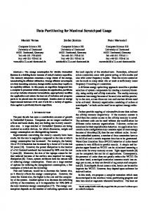
for arrays as discussed in [Li et al. 2005] and described in Section 2.2 below. Let us assume that the given SPM size is 320 bytes, which cannot hold all the five arrays at the same time. A live range splitting algorithm as introduced in [Li et al. 2005] and reviewed in Section 2.3 will be applied. This ensures that the data that are frequently accessed in a hot region can be potentially kept in SPM when that region is executed. We split an array (live range) accessed in hot loops (including call statements) where they are frequently accessed. (For convenience, a call statement that is not enclosed in a loop can be made so by assuming the existence of a trivial loop enclosing the call statement.) In Figure 1(b), the six oval blocks are the hot loops where live range splitting is performed. 2.2 Live Range Analysis An array is live at a program point if it may be used before redefined after that program point is executed. The live range of an array is the union of all program points in different functions where it is live. Due to the global nature of array live ranges, we have extended the liveness analysis for scalars to compute the live ranges of arrays inter-procedurally [Li et al. 2005]. To permit the data reuse information to be propagated across the functions in a program, we apply the standard liveness data-flow equations to the standard interprocedural CFG constructed for a program. Figure 2 shows the inter-procedural CFG and the live range information thus computed for Figure 1, where all interprocedural control flow edges are highlighted in gray. For convenience, we assume that every statement that causes an inter-procedural control flow (e.g., function call/returns and exceptional handling) forms a basic block by itself. As shown in Figure 2, the successor blocks of a call site are the unique ENTRY blocks of all functions that may be invoked at the callsite. Reciprocally, the successor blocks of a function’s unique EXIT block are the successor blocks of all its call sites. The predicates, DEF and USED, local to a basic block B for an array A are defined as follows. —USEDA (B) returns true if some elements of A are read (possibly via pointers) in B. We conservatively set USEDA (B) = true if an element of A may be read in B. —DEFA (B) returns true if A is killed in B. An array is killed if all its elements are redefined. In general, it is difficult to identify whether an array (i.e., every element of an array) has been killed or not at compile time. In the absence of such information, we have to conservatively assume that an array that appears originally in a program is killed only once at the entry of its definition block. In this paper, a definition block is referred to as a scope, e.g., a compound statement in C, where arrays are declared. Static-allocated arrays are defined at the outermost scope. In addition, an array introduced in live range splitting in a loop is defined at the entry of the loop where the splitting is performed (Section 2.3). Finally, for every edge connecting a call block and an ENTRY block, we assume the existence of a pseudo block C on the edge such that DEFA (C) returns true iff A is neither global nor passed by a parameter at the corresponding call site and USEDA (C) always returns false. This makes our analysis contextsensitive since if A is a local array passed by a parameter in one calling context to a callee, then its liveness information obtained at that calling context will not ACM Transactions on Embedded Computing Systems, Vol. ?, No. ?, 2010.

6

·

Li, Xue and Knoop A

B

C

D

E

int main() char A[80], B[75], *P; Entry BB1 BB3

BB2

BB4 void g(char *P) char C[120], D[120] ; BB6

Entry

BB5 Exit void f(char *P) char E[120] ;

Entry

BB7 BB8

BB9 BB10

Exit

Exit

Fig. 2. The live ranges of the four arrays after performing liveness analysis in the inter-procedural CFG in Figure 1, where the inter-procedural control flow edges are highlighted in gray.

be propagated into the other contexts for the same callee function. The liveness information for an array A can then be computed on the interprocedural CFG of the program by applying the standard data-flow equations to the entry and exit of every block B: LIVEINA (B) = (LIVEOUTA (B) ∧ ¬DEFA (B)) ∨ USEDA (B) _ LIVEOUTA (B) = LIVEINA (S) S∈succ(B )

(1)

where succ(B) denotes the set of all successor blocks of B in the CFG. For this particular example, the arrays A and B declared in main are used after the two call statements to g, respectively. As a result, both arrays are live through g and its callee f. The arrays C and D declared in g are live inside f since they are used after the two calls to f. E is only live in f. To understand the context-sensitivity of our analysis, let us consider a modified example of Figure 1 with BB4 and BB5 removed. Without context-sensitivity, the liveness results for the modified example are the same as those in Figure 2 (except that BB4 and BB5 are absent). With context-sensitivity, the live ranges of A and B are smaller: A is no longer live in BB3 and B is no longer live in BB2. This implies that the liveness information for the single parameter in each call site in the main function is only propagated back to the corresponding calling context. ACM Transactions on Embedded Computing Systems, Vol. ?, No. ?, 2010.

Scratchpad Memory Allocation via Interval Coloring

·

7

2.3 Live Range Splitting The intent is to keep in the SPM the data that are frequently accessed in a region when that region is executed. In embedded applications such as image processing, signal processing, video and graphics, most array accesses come from inside loops. We use the same splitting algorithm described in [Li et al. 2005] to split arrays at hot loops (including call sites as mentioned earlier) except that we also allow an array to be split even if it may be accessed by a pointer, which may also point to other arrays. This is realised by using runtime method tests that are often used for devirtualising virtual calls in object-oriented programs [Detlefs and Agesen 1999]. The basic algorithm for live range splitting is simple. The multiply nested loops in a function are processed outside-in to reduce array copy overhead. An array that can be split profitably in a loop will no longer be split inside any nested inner loop. Local arrays are split in the function where it is defined and global arrays may be split in all functions in the program. A simple cost model is used to decide if the live range of an array A in a loop L should be split into a new array A′ . Unnecessary splits may be coalesced during SPM allocation as described in Section 4. Due to splitting, an array copy statement A′ = A is inserted at the pre-header of L and A = A′ at every exit of L if A may be modified inside L and is live at the exit. All accesses to A (including those accessed indirectly by pointers) in L are replaced by those to A′ . So the cost of splitting A in L is estimated by (Cs + Ct × A.size) × copy f req, where Cs is the startup cost, Ct is the transfer cost per byte, A.size is the size of A and copy f req is the execution frequency of all such copy statements inserted for A. The benefit is A.freq × (Mmem − Mspm ), where A.freq is the access frequency of A in L, Mmem is the memory latency and Mspm is the SPM latency. If the benefit exceeds the cost, the split is performed. Due to the way that A′ is split from A in L, the live range of A′ is regarded as being live inside the entire loop, a good approximation for arrays as further discussed in Section 3. Figure 3 gives the modified program after live range splitting for our example. A, C, D and E are split at BB2, BB6, BB7 and BB9, respectively. B is split at both BB3 and BB5. (In BB5 shown in Figure 1(b), it is assumed that B is frequently accessed but A is not. So A needs not to be also split inside BB5.) As a result, all the memory accesses to these arrays in these blocks are redirected to the newly introduced live ranges A1, B1, B2, C1, D1 and E1 with array copy statements being inserted accordingly. Note that B is accessed via the pointer P in BB5. Thus, a runtime test is inserted at the entry of BB5 to redirect the pointer P to the new introduced array B2. Since P is not live at the exit of BB5, no runtime test is needed to redirect P to the original array B at the exit of BB5. Like garbage collectors, SPM allocators, which also reallocate array objects between the off-chip memory and the SPM, require some similar restrictions in programs, particularly those embedded ones written in C or C-like languages. These are the restrictions that should be satisfied for live range splitting to work correctly. Programming practices that disguise pointers such as casts between pointers and integers are forbidden. In addition, only portable pointer arithmetic operations on pointers and arrays are allowed. In general, C programs that rely on the relative positions of two arrays in memory are not portable. Indeed, comparisons (using, ACM Transactions on Embedded Computing Systems, Vol. ?, No. ?, 2010.

8

·

Li, Xue and Knoop int main() char A[80], B[75], *P; Entry BB1
 
 if () BB3

BB2

call g(A1)

call g(B1)







BB4 P = A or B void g(char *P) char C[120], D[120] ; Entry 
  BB6 for () if () call f(C1)   

  BB7 for () if () call f(D1)   
BB8 P[...]=C[...]+D[...] Exit

BB5

for()  = *P++;

     

Exit void f(char *P) char E[120] ; Entry 
 

BB9 for () E1[] =    
BB10 P[...] = E[...] Exit

Fig. 3. The modified program after live range splitting for the example in Figure 1. The six hot blocks where splitting takes place are highlighted in gray. B is accessed indirectly via pointer P in BB5. The runtime test inserted at the entry of BB5 checks whether P points to B or not.

e.g., < and 6) and subtractions on pointers to different arrays are undefined or implementation-defined. Also, if n is an integer, p ± n is well-defined only if p and p ± n point to the same array. Fortunately, these restrictions are usually satisfied for static arrays and associated pointers in portable ANSI-compliant C programs. In this paper, an array A in a loop L is split only if all pointers to A in L are scalar pointers that point directly to A. (This implies that A in L cannot be pointed to by fields in aggregates such as heap objects or arrays of pointers or indirectly by scalar pointers to pointers.) For such an array, code rewriting, as demonstrated in Figure 3, required by splitting the array can be done efficiently at the pre-header and exits of the loop. In all embedded C benchmarks we have seen (including those used here), static arrays are generally splittable as validated in Figure 13. All the arrays that appear originally in a program before live range splitting is applied are referred to as original arrays. We write Aorg to denote the set of all these original arrays. All new arrays introduced inside loops are called hot arrays. All the loops that contain at least one hot array are called hot loops. We write Ahot to denote the set of all hot arrays. In our example, there are five original arrays: Aorg = {A, B, C, D, E}. All these arrays, except for array B, happen to have been split exactly once each and B has been split twice. So there are six hot arrays: Ahot = {A1, B1, B2, C1, D1, E1}. In particular, A1, B1, B2, C1, D1 and E1 are hot arrays introduced in hot loops BB2, BB3, BB5, BB6, BB7 and BB9, respectively. Recall that, for convenience, hot call sites are also referred to as hot loops. ACM Transactions on Embedded Computing Systems, Vol. ?, No. ?, 2010.

Scratchpad Memory Allocation via Interval Coloring A

B

C

D

E

A1 B1 B2 C1 D1 E1

·

9

int main() char A[80], B[75], *P; Entry BB1 BB3

BB2

BB4 void g(char *P) char C[120], D[120] ; BB6

Entry

BB5 Exit void f(char *P) char E[120] ; Entry

BB7 BB8

BB9 BB10

Exit

Exit

Fig. 4. Live ranges for the five original arrays in Aorg = {A, B, C, D, E} and the six hot arrays Ahot = {A1, B1, B2, C1, D1, E1} after live range splitting for the example in Figure 1.

Figure 4 illustrates the live ranges for both original and hot arrays in our example. The live ranges of the five original arrays remain the same as in Figure 2. As for the six hot arrays, A1 is live in BB2 and the callee functions f and g invoked in BB2. B1 is live in BB3 and the callees f and g. B2 is only live in BB5. C1 is live in BB6 and the callee f. D1 is live in BB7 and the callee f. E1 is only live in BB9. 2.4 Interval Coloring The goal of SPM allocation is to find a way to map arrays into either SPM or off-chip memory. An SPM allocator needs to decide which arrays should be placed in SPM and where each SPM-resident array should be placed in SPM. When live range splitting is applied, it also should coalesce some unnecessary splits since live range splitting is usually performed optimistically in register/SPM allocation. Definition 1. The set, Acan , of candidates for SPM allocation is Aorg ∪ Ahot . As will be explained in Section 4.2, either an original array is considered for SPM allocation or all the hot arrays split from it but not both at the same time. In this paper, the SPM allocation problem is modelled as an interval coloring problem for an array interference graph built from a program. Figure 5 gives two example interference graphs for the program in Figure 4, where the weight of an array node is the size of the array. One array is said to interfere with another if it is defined at a program point where the other is live. In a strict program where there ACM Transactions on Embedded Computing Systems, Vol. ?, No. ?, 2010.

10

·

Li, Xue and Knoop 80

80 A1

A

75

75

120 C

B

120

B1

C1

75 B2 D

E

D1

E1

120

120

120

120

(a) Original arrays in Aorg

(b) Hot arrays in Ahot

Fig. 5. Two example interference graphs using the arrays from the example program in Figure 1.

is a definition of a variable on any static control path from the beginning of the program to a use of this variable, this criterion is equivalent to that two variables interfere if their live ranges intersect [Bouchez et al. 2007]. However, for the arrays in an inter-procedural CFG, the corresponding program may not be strict due to array accesses via aliased pointers in different functions. In our example given in Figure 4, A1 and B1 do not interfere with each other even though both are live in function f. Thus, we prefer to use the more relaxed interference criterion of Chaitin [Chaitin 1982]: two arrays interfere if the live range of one array contains a definition of the other. Any pair of interfering arrays are connected by an edge in an interference graph to indicate that they cannot be allocated to overlapping SPM spaces. The interval coloring problem is thus defined as follows. Definition 2. Given a node weighted graph G = (V, E) and positive-integral vertex weights w = V → N, the interval coloring problem for G seeks to find an assignment of an interval Iu to each vertex u ∈ V , i.e., a valid coloring G i such that two conditions are satisfied: (1) for every vertex u ∈ V , |Iu | = wu and (2) for every pair of adjacent vertices u, v ∈ V , Iu ∩ Iv = ∅. S The goal of interval coloring is to minimise the span of intervals | v∈V Iv | required in a valid coloring. When every node in the graph G has a unity weight, the interval coloring problem degenerates into the traditional graph coloring problem. Interval coloring provides a natural formulation for the SPM allocation problem. Allocating SPM spaces to arrays is accomplished by assigning intervals to the nodes in the graph. Minimising the span of intervals amounts to minimising the required SPM size. The decision concerning whether to actually split an array or not can be integrated into an SPM allocator as a coalescing problem during coloring. 3. ARRAY INTERFERENCE GRAPHS AS SUPERPERFECT GRAPHS Let us firstly recall some standard definitions for a node weighted graph G: —A clique in G is a complete subgraph of G. A clique in G is a maximal clique if it is not contained in any other clique in G. The order of a clique is the sum of the weights of all nodes in the clique. Since the weights of nodes are positive, a maximum clique in G is a (maximal) clique in G with the largest order. —The chromatic number of G is the minimal span of intervals needed to color G. ACM Transactions on Embedded Computing Systems, Vol. ?, No. ?, 2010.

Scratchpad Memory Allocation via Interval Coloring A

A

B

B

Fig. 6.

11

A

B

(a) Containing-related

·

(b) Non-interfering

(c) Interfering

Containing-related, non-interfering and interfering array live ranges for A and B.

—The clique number of G is the order of a maximum clique in G. In general, the chromatic number of a node weighted graph is equal to or greater than its clique number. A graph G is known as a superperfect graph if for any positive weight function defined on G, the chromatic number of G is always equal to the clique number of G. (A graph is a perfect graph if its chromatic number is equal to its clique number when all its nodes have unity weights.) As noted earlier, how to recognise and color superperfect graphs is open [Golumbic 2004]. In Section 3.1, we provide evidence to show that in many embedded C applications, two arrays are often containing-related when they interfere with each other. In Section 3.2, we show that array interference graphs are comparability graphs if their array live ranges do not interfere or are containing-related. This gives rise to an efficient procedure (given in Algorithm 9) for finding optimal colorings for this special class of superperfect graphs. This, in turn, motivates the development of our interval-coloring algorithm for SPM allocation to be described in Section 4. 3.1 Containment As illustrated in Figure 6, two array live ranges can be related in one of the three ways. Consider our example in Figure 4, hot arrays A1 and B1 do not interfere since neither is live at any program point where the other is defined. However, A1 contains C, which implies A1 interferes with C, since A1 is live at all program points where C is (including the point at which C is defined). In this example as well as many embedded programs we have studied, the situation depicted in Figure 6(c) happens only rarely. Frequently, Property 1 holds for two arrays (i.e., two original or hot arrays in Acan given in Definition 1). Property 1. A program has the so-called containment property if whenever the live ranges of two arrays in Acan in the program interfere, then the live range of one array contains that of the other. As a result, any two arrays in a program either do not interfere or are containingrelated. In Section 2.2, we mentioned that an array in a program is conservatively assumed to be defined only once at its definition block, i.e., the scope where it is defined. By convention, global arrays are defined in the outermost scope in the program. By construction, hot arrays are defined at the entry of hot loop blocks where they are split. By Definition 1, the SPM candidates are the original arrays in Aorg and all ACM Transactions on Embedded Computing Systems, Vol. ?, No. ?, 2010.

12

·

Li, Xue and Knoop

hot arrays in Ahot . So we only need to consider these live ranges below. Assumption 1. For two arrays defined in a common definition block, every last use of one array must be post-dominated by at least one last use of the other. Assumption 2. If an array defined in a definition block is live at the entry of an inner definition block, then it is live at the exit(s) of, i.e., through the inner block. Assumption 3. If an array is live at the entry of a call site, then it is live at the exit(s) of the call site (i.e., live through all invoked callee functions at the site). Assumption 1 is applicable to the arrays defined in a common definition block. These arrays are mutually interfering since their definition sites start from the entry of the same definition block. Assumptions 2 and 3 are seemingly restrictive; but they do not warrant relaxation for three reasons. First, the local arrays in a function are usually declared in its outermost scope in embedded applications. Second, a hot array is live only in the scope defined by the hot loop where it is split. Third, we have studied the live range behaviour in a set of 17 representative embedded C applications from MediaBench and MiBench benchmark suites (Table I). Only four arrays in pegwitencode and pegwitdecode do not satisfy these three assumptions. Theorem 1. Property 1 holds if Assumptions 1 – 3 are all satisfied. Proof. Let A and B be any two interfering arrays in the program. If both are defined in the same definition block, then one must contain the other by Assumption 1. Otherwise, let A be defined in a scope that includes the scope in which B is defined. By Assumption 2, A must contain B in the absence of function calls in the program. When there are function calls in the program, we note that Assumption 3, which takes care of the arrays defined in different functions, is identical to Assumption 2 since a callee function made in a caller function, once inlined conceptually in the caller, represents an inner scope nested in the caller. Definition 3. G is said to be containing-related if it satisfies Property 1. 3.2 Recognition and Coloring We show that containing-related interference graphs form a special class of superperfect graphs known as comparability graphs and their optimal colorings can thus be found efficiently. Let G be a node weighted undirected graph. An acyclic orientation G o of G seeks to find an assignment of a direction or orientation to every edge in G so that the resulting graph is a DAG (directed acyclic graph). It is well-known that there exists a one-to-one correspondence between the set of interval colorings of G (given in Definition 2) and the set of acyclic orientations of G. For every edge (x, y) in G, x is located to the left of y in an interval coloring G i of G if and only if (x, y) is a directed edge in an acyclic orientation G o of G. An acyclic orientation G o of G is transitive if (x, z) is contained in G o whenever (x, y) and (y, z) are. G is known as a comparability graph if a transitive orientation of G exists. We write A ⊒ B if A contains B. The following lemma says that ⊒ is transitive. Lemma 1. If A ⊒ B and B ⊒ C, then A ⊒ C. Proof. Note that we use the interference criterion of Chaitin [Chaitin 1982] in this work. If A ⊒ B, then the live range of A includes that of B, which must ACM Transactions on Embedded Computing Systems, Vol. ?, No. ?, 2010.

·

Scratchpad Memory Allocation via Interval Coloring

13

 

&'!( )!  *"



%

 

  

#!  $

  !"

Fig. 7.

An interval-coloring-based SPM allocator IC.

contain a definition of B. Similarly, if B ⊒ C, then the live range of B includes that of C, which must contain a definition of C. Hence, A ⊒ C. Let G0 be a graph with n nodes v1 , v2 , . . . , vn and G1 , G2 , . . . , Gn be n disjoint undirected graphs. The composition graph G = G0 [G1 , G2 , . . . , Gn ] is formed in two steps. First, replace vi in G0 with Gi . Second, for all 1 ≤ i, j ≤ n, make each node of Gi adjacent to each node of Gj whenever vi is adjacent to vj in G0 . Formally, for G i = (Vi , Ei ), the composition graph G= (V, E) is defined as follows: V = ∪16i6n Vi E = ∪16i6n Ei ∪ {(x, y) | x ∈ Vi , y ∈ Vj and (vi , vj ) ∈ E0 }

(2) (3)

The following result about the recognition of composition graphs as comparability graphs from their constituent components is recalled from [Golumbic 2004]. Lemma 2. Let G = G0 [G1 , G2 , . . . , Gn ], where each Gi (0 ≤ i ≤ n) is a disjoint undirected graph. Then G is a comparability graph if and only if each Gi is. Theorem 2. If G is containing-related, then G is a comparability graph. Proof. Let us write A ≡ B if two interfering arrays A and B have the identical live range, i.e., if A ⊒ B and B ⊒ A. Let G 1 , G 2 , . . . , G n be all n maximal cliques of G such that for every G i (1 6 i 6 n), every pair of array nodes A and B in G i are such that A ≡ B. Let G 0 be obtained from G with each G i collapsed into one node. Then G = G 0 [G 1 , G 2 , . . . , G n ]. G 0 must be a comparability graph. To see this, let X and Y be two nodes in G 0 , each of which may represent a set of array nodes in G. Let AX (BY ) be an array represented by X (Y ). An acyclic orientation of G 0 is found if AX is made to be directed to BY whenever AX ⊒ BY . In addition, this orientation is transitive by Lemma 1. Note that every G i is trivially a comparability graph since it is a clique. Hence, G is a comparability graph by Lemma 2. Given a transitive orientation G o of a comparability graph G, we can obtain an optimal interval coloring in linear time by a depth-first search. For a source node x in G o , let its interval be Ix = [0, w(x)), where w(x) is the weight of x. Proceeding inductively, for a node y with all its predecessors already being colored, let t be the largest endpoint of the intervals of these predecessors and define Iy = [t, t + w(y)). This algorithm is used in our SPM allocator as discussed in Section 4.3. ACM Transactions on Embedded Computing Systems, Vol. ?, No. ?, 2010.

14

·

Li, Xue and Knoop

4. INTERVAL-COLORING-BASED SPM ALLOCATION Motivated by the facts that array interference graphs are often containing-related (Section 3.1) and containing-related interference graphs are comparability graphs and can thus be efficiently colored (Section 3.2), Figure 7 outlines our IC algorithm with its three phases described below and then explained in detail afterwards. The first phase, Superperfection, constructs a containing-related array interference graph G can from Acan (Section 4.1). The middle phase, Spill & Coalesce (Section 4.2), addresses the two inter-related problems concerning which arrays can be placed in SPM (Spill) and which arrays should be split (Coalesce) in the current interference graph G under consideration, which is always a node-induced subgraph of G can and thus a comparability graph itself. (A node-induced subgraph of a graph G is one that consists of some of the nodes of G and all of the edges that connect them in G.) If the size of a given SPM is no smaller than the clique number of G, then the middle phase is not needed. In this case, G can be optimally colored immediately. Otherwise, some heuristics motivated by containing-related interval coloring are applied to split and spill some array live ranges in G until the resulting graph can be optimally colored. The last phase, Coloring, places all SPM-resident arrays in SPM (Section 4.3). In existing graph coloring allocators for scalars [George and Appel 1996; Park and Moon 2004] and for arrays [Li et al. 2005], live range splitting is usually performed aggressively first and then unnecessary splits are coalesced during coloring. This paper proposes to make both splitting and spilling decisions together during Spill & Coalesce based on a unified cost-benefit analysis as motivated in Section 4.2.1 and illustrated in Section 4.4. Our cost-benefit analysis is performed by examining the changes to the maximal cliques in the current interference graph G caused by a splitting or spilling operation. We deduce these changes efficiently from the maximal cliques constructed (only once) from G can . When both splitting and spilling operations are performed together, the Spill & Coalesce phase may look slightly complex. However, better SPM allocation results are obtained as validated here. 4.1 Superperfection Given the set Acan of SPM candidates (Definition 1), we apply Algorithm 1 to build a containing-related interference graph G can from Acan . Since containment implies interference, i.e., if A ⊒ B, then A and B interfere with each other, we will represent a containing-related interference graph G as a DAG. A directed edge A → B in G means A ⊒ B. In addition (as demonstrated in the proof of Theorem 2), all arrays with the same live range are collectively represented by one node. In other words, if A ⊒ B and B ⊒ A, then A and B are represented by the same node. Furthermore, we have also decided not to represent explicitly the transitive edges (as characterised in Lemma 1) in G for three reasons. First, the absence of transitive edges in G makes it easier to find all its maximal cliques as shown in Algorithm 3. Second, our IC algorithm checks efficiently the existence of interference between two arrays by examining if both are in the same maximal clique rather than if both are connected by a containment edge. Third, the interference graphs without transitive edges are simpler and visually cleaner. Figure 8 gives the DAG representations of the two interference graphs in Figure 5. ACM Transactions on Embedded Computing Systems, Vol. ?, No. ?, 2010.

Scratchpad Memory Allocation via Interval Coloring

15

80 A1

155 A B 75

120

B1

240 C D

·

C1

75 B2

E

D1

E1

120

120

120

(a) Original arrays in Aorg Fig. 8.

(b) Hot arrays in Ahot

DAG representations of the two interference graphs given in Figure 5.

Algorithm 1 Building a containing-related interference graph G can from Acan . 1: procedure Build(Acan ) 2: The nodes in G can are the arrays in Acan 3: for every function f in the program do 4: for every scope S in function f do // Lines 5 – 12 to enforce Assumption 1 5: for every two arrays in Acan defined in S do // both must interfere 6: if the two arrays, A and B, are containing-related then 7: Add A → B if A ⊒ B and B → A if B ⊒ A 8: else 9: Denote them A and B such that A is less frequently accessed 10: Add A → B 11: end if 12: end for // Lines 13 – 17 to enforce Assumptions 2 and 3 13: for every B ∈ Acan defined in S do 14: for every A ∈ Acan that is live but not defined in S do 15: Add A → B 16: end for 17: end for 18: end for 19: end for 20: Collapse every SCC (Strongly-Connected Component) of G can to one node 21: Let all transitive edges of G can be removed via a transitive reduction to G can 22: return G can 23: end procedure

Algorithm 1 builds G can (a DAG) for all the arrays in Acan in a program (line 2). As discussed in Section 2.2, every array is assumed conservatively to be defined at the entry of its definition block. Therefore, we only need to examine the program points where some arrays are defined (lines 5 and 13). In lines 5 - 12, we consider the array live ranges defined in a common scope, which must all interfere with each other. If the two interfering arrays A and B are not containing-related (lines 8 – 11), we enforce Assumption 1 by making the one that is less frequently accessed ACM Transactions on Embedded Computing Systems, Vol. ?, No. ?, 2010.

16

·

Li, Xue and Knoop 120 75

B2

80

E

A

155 A B

80 A1

75

120

B

C

B1

C1

75

120 D 120

E1 120

D1 120

(a) Traditional representation

80 A1

B1 75

B2 75

C D 240 120 C1

D1 120 E 120 E1 120

(b) DAG constructed by Build

Fig. 9. Traditional and DAG representations of the interference graph built from Acan in Figure 4.

contain the other. The intuition behind is to avoid extending the live ranges of frequently accessed arrays so they may have a better chance to be placed in SPM. In lines 13 – 17, we examine every pair of interfering arrays A and B defined in two different scopes. Line 15 serves a double purpose: if A ⊒ B, we need to add A → B to G can . Otherwise, we enforce A → B (Assumptions 2 and 3). Live range extension is a safe and conservative approximation of liveness information. For the set of 17 embedded C applications we have studied (Table I), only four live ranges in pegwitencode and pegwitdecode are extended (Section 3.1). In line 20, all array nodes with the same live range are merged. In line 21, all transitive edges in G can are removed by performing a standard transitive reduction on G can . Algorithm 1 is correct in the sense that after line 19, every pair of interference edges in the program is included in G can due to lines 5 and 13 – 14 and every interference edge is containing-related due to lines 7, 10 and 15. In Figure 4, all eight arrays in Acan either do not interfere or are containingrelated. No live range extension is necessary. Figure 9 gives the interference graph built from Acan . By comparing the traditional and our DAG representations, the DAG representation (due to the exploitation of containment) is simpler. 4.2 Spill & Coalesce Our algorithm performs spilling and splitting together based on a cost-benefit analysis, which examines the resulting changes to the maximal cliques in the interference graph G. To help understand our algorithm, we will first motivate our approach in Section 4.2.1 by focusing on these two aspects using the example given in Figure 1. We will then describe our algorithm in detail in Sections 4.2.2 – 4.2.6. The set of SPM candidates Acan = Aorg ∪ Ahot is given in Definition 1. During SPM allocation, either an original array A ∈ Aorg is a candidate or all its corresponding hot arrays A1 , A2 , . . . , An ∈ Ahot are but not both at the same time. Note that it is possible that only some but not all of these hot arrays are eventually colored. Note also that A and all its hot arrays may be coalesced if A turns out to be colorable entirely later (due to spilling and splitting performed to other arrays). When A is split, all its hot arrays A1 , A2 , . . . , An will become candidates and the non-hot live range of A is spilled. Among the 17 benchmarks used in our experiments, the non-hot portions of the array live ranges in each of these benchmarks ACM Transactions on Embedded Computing Systems, Vol. ?, No. ?, 2010.

Scratchpad Memory Allocation via Interval Coloring 80 A1

80 A1

B1 75

B2 75

B1 75 C 120

80 A1

120

C1

C D 240

D1 120

E 120

E 120

(a) Splitting A and B from Figure 8(a). Fig. 10.

B2 75

B1 75

·

17

B2 75

120 D1

E 120

(b) Splitting D and then C from (a)

80 A1

B1 75

B2 75

C 120 E 120

(c) Spilling D from (a)

Interference graphs of the candidate arrays after splitting or spilling.

account for less than 5% of the total number of array accesses. The performance improvement from allocating them to SPM (if possible) is often negligible. For an array A, we write HOTA to denote the set of all hot arrays from A. If A is an original array that cannot be split or a hot array, we define HOTA = ∅. This notational convenience has helped in simplifying the presentation of Algorithms 6 – 8 (by allowing us to treat all arrays in Acan in a unified manner). We write SPM SIZE to denote the size of the SPM under consideration. 4.2.1 Motivation. The interference graph G can constructed by Build from Acan = {A,B,C,D,E,A1,B1,B2,C1,D1,E1} is given in Figure 9. Recall that Aorg = {A,B,C,D,E}. Their array sizes are: A.size=80, B.size=75 and C.size=D.size=E.size=120. All five arrays are split as shown in Figure 4. So Ahot = {A1,B1,B2,C1,D1,E1}. The array sizes of these hot arrays are the same as their corresponding original arrays. 4.2.1.1 Cost-Benefit Analysis. To avoid introducing too many unnecessary splits a priori, we propose to perform splitting on-demand during coloring based on a cost-benefit analysis. In the literature, splitting is usually considered to be less expensive than spilling. However, this assumption is not always true. For our example, our algorithm starts with the five candidates in Aorg = {A,B,C,D,E} with their interference graph G being given earlier in Figure 8(a). Suppose that the size of SPM is 320 bytes, which is not large enough to hold all the five arrays. Suppose that instead of A and B, their hot arrays A1, B1 and B2 as shown in Figure 3 are considered next for SPM allocation. The updated interference graph G is shown in Figure 10(a). However, the SPM is still not large enough to hold all the arrays in {A1,B1,B2,C,D,E}. Splitting D and then C as suggested in Figure 3 will result in the interference graph as shown in Figure 10(b). On the other hand, spilling D will give rise to the interference graph in Figure 10(c). The two resulting interference graphs can both be colored. If the profit of spilling D is higher than the profit of splitting D and C together, then spilling D is better, a solution that cannot be found if splitting is always preferred to spilling blindly. The above-mentioned problem arises because existing SPM allocators make their splitting and spilling decisions without considering their relative costs and benefits carefully. Let G be the current interference graph formed by the array candidates being considered. The benefit of splitting or spilling an array should represent the increased possibility for the other arrays to be colored, i.e., the increased colorability of the other arrays. We use a simple yet intuitive model to evaluate the colorability of an array A in G. If A can be simplified, i.e., is guaranteed to be colorable, we ACM Transactions on Embedded Computing Systems, Vol. ?, No. ?, 2010.

18

·

Li, Xue and Knoop

Algorithm 2 Cost-benefit analysis for estimating the profit of spilling/splitting. 1: procedure CBAforSpill(G := V, E), A) 2: G new = G ⊖ {A} (interference graph formed by V \ {A}) 3: A.spill cost = A.freq × (Mmem − Mspm ) 4: A.spill benefit = (α(G new ) − α(G)) × (Mmem − Mspm ) 5: A.spill profit = A.spill benefit − A.spill cost 6: return A.spill profit 7: end procedure 8: procedure CBAforSplit(G := V, E), A) 9: G new = G ⊖ {A} ⊕ HOTA (interference graph formed by (V \ {A}) ∪ HOTA ) 10: A.split cost is the array copy cost plus the cost incurred for accessing the non-hot portions of A from off-chip memory (Sect. 2.3) 11: A.split benefit = (α(G new ) − α(G)) × (Mmem − Mspm ) 12: A.split profit = A.split benefit − A.split cost 13: return A.split profit 14: end procedure have colorability(G, A) = 1. Otherwise, its colorability is estimated by: colorability(G, A) =

SPM SIZE 6 1 Θ(G, A)

(4)

where Θ(G, A) is the largest order possible for a maximal clique containing A found in G, indicating the minimum amount of space required to color all arrays in the clique. In other words, colorability(G, A) approximates the (average) percentage of accesses to A that may hit in SPM after a coloring has been found. Consider Figure 10(a) with SPM SIZE = 320 bytes. There are three maximal cliques: {A1,C,D,E}, {B1,C,D,E} and {B2} with their orders being 440, 435 and 75, respectively. The two larger cliques cannot be colored. Hence, colorability(G, A1) = 320 colorability(G, C) = colorability(G, D) = colorability(G, E) = 440 and 320 colorability(G, B1) = 435 . Since B2 can be colored, colorability(G, B2) = 1. We use α(A) to approximate the number of array accesses of A that may hit in SPM after SPM allocation (with A.freq being the access frequency of A): α(A) = A.freq × colorability(G, A) = A.freq ×

SPM SIZE Θ(G, A)

As a result, the number of the array accesses that can hit in SPM for all arrays in G after SPM allocation is the sum of their α values: X α(G) = α(A) (5) Array A contained in G The larger α(G) is, the better the allocation results for G will (potentially) be. Algorithm 2 gives our cost-benefit analysis for estimating the profit of splitting and spilling A in G, where Mmem and Mspm are defined in Section 2.3. In lines 2 and 9, the operations ⊖ and ⊕ for updating G = (V, E) with S ⊂ Acan are defined ACM Transactions on Embedded Computing Systems, Vol. ?, No. ?, 2010.

Scratchpad Memory Allocation via Interval Coloring

·

19

by: G ⊖ S = subgraph of G can induced by V \ S G ⊕ S = subgraph of G can induced by V ∪ S

(6) (7)

These operations, which will be used later in Algorithms 6 and 8, together with those on α in lines 4 and 11, can be performed efficiently as explained shortly below. In CBAforSpill, the cost of spilling A from G is estimated by the increased number of cycles when the spilled A is potentially relocated from the SPM to the off-chip memory. The benefit is the number of cycles reduced due to an improvement on the colorability values of the other arrays. In CBAforSplit, the cost of splitting A into the hot arrays in HOTA in G is calculated according to the live range splitting algorithm described in Section 2.3. The benefit is similarly estimated as for spilling. Let us explain our cost-benefit analysis by using the example given in Figure 10(a). As before, SPM SIZE = 320. Recall that the colorability for each array 320 , the colorability of B1 is 320 in {A1, C, D, E} is 440 435 and the colorability of B2 is 1. Let us first look at the cost and benefit of spilling D with G being updated from Figure 10(a) to Figure 10(c). In line 3, we have D.spill cost = D.freq × (Mmem − Mspm ). After spilling, all arrays can be simplified and their colorability values are 320 1. In line 4, we get D.spill benefit = ((A1.freq+C.freq+E.freq)×(1− 440 )+B1.freq× 320 profit as ) − D.freq × 320 ) × (M − M ). In line 5, we obtain D.spill (1 − 435 mem spm 440 desired. Let us divert slightly by considering to spill A1 instead of D in Figure 10(a). After spilling, there are two maximal cliques {B1,C,D,E} and {B2} with their orders being 435 and 75, respectively. Thus, the colorability values of C, D and E have improved 320 320 from 440 to 435 . In line 3, we have A1.spill cost = A1.freq×(Mmem −Mspm ). In line 320 4, we obtain A1.spill benefit = ((C.freq+D.freq+E.freq) × ( 320 435 − 440 ) − A1.freq × 320 440 ) × (Mmem − Mspm ). In line 5, we obtain A1.spill profit as desired. If all arrays have the same access frequency, then D is preferred to A1 for spilling since spilling D has a higher profit. Let us next look at the cost and benefit of splitting D into D1 with G being updated from Figure 10(a) to Figure 10(b). For now, this splitting operation (shown in Figure 3) is not profitable since it does not change the colorability of the other 320 arrays. In line 11, we get D.split benefit = −Dno−hot .freq× 440 ×(Mmem −Mspm ). In line 10, we have D.split cost = 2 × (Cs + Ct × D.size) × copy f req + Dno−hot .freq × (Mmem − Mspm ), where Cs , Ct and copy freq are introduced in Section 2.3 and Dno−hot represents the not-hot part live range of D. Finally, we obtain C.split profit in line 12 as desired. If we subsequently split C, then the colorability of all arrays in the resulting interference graph remain unchanged. So a similar cost-benefit analysis as that for D applies. Let us assume that we are to decide whether to split or spill D in Figure 10(a). If D.split profit is larger than D.spill profit, then D is selected for splitting as shown in Figure 10(b). Otherwise, D is spilled as shown in Figure 10(c). 4.2.1.2 Updating Interference Graph. From the above discussions, we can see that the interference graph G must be updated when computing the benefit of a splitting or spilling operation. As reflected in lines 2 and 9 in Algorithm 2, G evolves into G new when A is spilled or split. To compute its benefit (in lines 4 and ACM Transactions on Embedded Computing Systems, Vol. ?, No. ?, 2010.

20

·

Li, Xue and Knoop

Algorithm 3 Finding maximal cliques in a containing-related interference graph. 1: procedure FindMaxCliques(G := (V, E)) 2: Let S be the set of source nodes in G without any incoming edges 3: Let T be the set of sink nodes in G without any outgoing edges 4: let P(s, t) be a path from s ∈ S and t ∈ T . 5: C = {c | c is a set of nodes in G found in P(s, t), where s ∈ S and t ∈ T } 6: for every A ∈ V do 7: A(G).MaxCS = {c ∈ C | c contains A} 8: end for 9: end procedure

11 in Algorithm 2), we need to recompute Θ(G new , B) for all and only the arrays B in update(A) such that Θ(G new , B) 6= Θ(G, B) may hold. In the case of spilling, update(A) is the set of arrays B that interfere with A. In the case of splitting, update(A) also includes the hot arrays in HOTA . Our solution is simple and has been engineered to be efficient for real programs with array candidates. We call FindMaxCliques(G can ) in Algorithm 3 (only once) to initialise A(G can ).MaxCS with the set of all maximal cliques containing A in G can . There is no need to call FindMaxCliques(G) any more for the current interference graph G to recompute A(G).MaxCS every time G is updated. Instead, the information required can be derived efficiently from A(G can ).MaxCS. Let A(G can ).MaxCS ↓ G = { the sub-clique of c induced by the nodes of c that are also in G | c ∈ A(G can ).MaxCS}. Since G can is a comparability graph, all its node-induced subgraphs G are also comparability graphs. Then we must have A(G).MaxCS ⊆ A(G can ).MaxCS ↓ G and A(G can ).MaxCS ↓ G \ A(G).MaxCS contains cliques of A in G. Thus, the largest order of a maximal clique containing A in G can be found from A(G can ).MaxCS ↓ G incrementally as discussed below. In our implementation, an array in Acan is said to be active if it is presently a candidate in G and inactive otherwise. Whether an array is active or inactive is marked as such (with a Boolean flag) in the A(G can ).MaxCS sets for all arrays A ∈ Acan . Whenever an array A is spilled or split in G, A is marked as inactive, and in the case of splitting, all those in HOTA are marked as active. This realises efficiently the graph updating operations performed in lines 2 and 9 in Algorithm 2 and other parts of our IC algorithm. To compute the benefit of spilling or splitting A from G to obtain G new in lines 4 and 11 in Algorithm 2, we need only to recompute Θ(G new , B) for the arrays B in update(A), which is found simply as the set of active arrays that appear in A(G can ).MaxCS. Finally, Θ(G new , B) can be obtained efficiently from B(G can ).MaxCS ↓ G new for every array B ∈ update(A). In the worst case, G can can have an exponential number of maximal cliques in terms of the number of nodes in G can . However, as shown in Table II, for all benchmarks we have tested, the largest number of maximal cliques is 267. In addition, FindMaxCliques(G can ) is called only once. Finally, incrementally updating the maximal cliques for G integrates smoothly with the overall iterative-coalescing framework. More importantly, our IC algorithm is efficient as shown in Table III. ACM Transactions on Embedded Computing Systems, Vol. ?, No. ?, 2010.

Scratchpad Memory Allocation via Interval Coloring

·

21

Algorithm 4 Interval-coloring-based SPM allocation. 1: procedure IC(G can ) 2: FindMaxCliques(G can ) 3: Init() 4: repeat 5: if UnSpillList 6= ∅ then 6: UnSpill() 7: else if SplitOrSpillList 6= ∅ then 8: SplitOrSpill() 9: end if 10: until UnSpillList = ∅ ∧ SplitOrSpillList = ∅ 11: end procedure Algorithm 5 Initialising the (current) interference graph and worklists. 1: procedure Init 2: Let G be the subgraph of G can induced by Aorg 3: UnSpillList = ∅ 4: RemoveList = ∅ 5: SplitOrSpillList = set of arrays A in G s.t. Θ(G, A) > SPM SIZE} (Def. 4) 6: end procedure 4.2.1.3 Overview. Like George and Appel’s graph coloring allocator for scalars [George and Appel 1996], IC is also an worklist-based iterative-coalescing allocator (but for data aggregates). So the operational flows among the five modules in this middle phase IC shown in Figure 7 are captured in Algorithm 4. The meanings of the three lists, UnSpillList, SplitOrSpillList and RemoveList and which arrays are eventually identified to be SPM-resident are explained in Section 4.2.2. Our IC allocator is developed based on the following observation. Definition 4. An array in G can be simplified, i.e., guaranteed to be placed in SPM if it is not included in a clique in G with an order larger than the SPM size. Theorem 3. G can be colored iff all arrays in G can be simplified. Proof. Follows from Definition 4 and Theorem 2. Since simplified arrays can always be colored, no splitting for an original array is necessary if it can be simplified in G can that is built directly from Acan . 4.2.2 Init. In Algorithm 5, the current interference graph G that IC starts with is initialised (line 2). So are the three worklists, which are central to IC, a worklistbased iterative-coalescing algorithm (lines 3 – 5). Below we describe these data structures in detail. An illustration of these lists using our running example can be found in Section 4.4. However, due to the iterative nature of IC, these worklists may have to be understood (dynamically) in the iterative-coalescing context. UnSpillList and RemoveList are initialised to be empty and SplitOrSpillList to contain all arrays in G that cannot be presently simplified (i.e.,, colored). . SplitOrSpillList contains arrays in G that cannot be simplified by Definition 4. ACM Transactions on Embedded Computing Systems, Vol. ?, No. ?, 2010.

22

·

Li, Xue and Knoop

These are the candidates considered for splitting and spilling. . RemoveList contains arrays in G can but not in G that are potentially spilled. These are removed (i.e. spilled) from either SplitOrSpillList or UnSpillList. Every array is not simplifiable at the time when it is added to this list. However, some arrays in the list may become simplifiable after others have been split or spilled. . UnSpillList contains arrays in G can but not in G that are transferred from RemoveList to this list when they become simplifiable (as discussed above). These are the candidates that may be unspilled, i.e., added back to G. However, unspilling one array in this list may cause others in the list to become non-simplifiable. All such non-simplifiable arrays will be removed and added back to RemoveList. At any time, the three lists are mutually exclusive. In addition, SplitOrSpillList contains either A or its hot arrays in HOTA but not both. This is because only A or its hot arrays in HOTA are considered for SPM allocation at any time. However, RemoveList and UnSpillList may contain both A and its hot arrays in HOTA at the same time. In the case of RemoveList, once A is spilled to the list, some of its hot arrays may also be spilled to the list immediately afterwards. In the case of UnSpillList, if A may not be unspilled, some of its hot arrays may be unspilled. The Spill & Coalesce phase terminates when both SplitOrSpillList and UnSpillList are empty. Then G contains all the arrays that can be placed in SPM. This phase is guaranteed to terminate since IC works by reducing the clique number of G gradually until it is smaller than or equal to SPM SIZE. 4.2.3 UnSpill. When Algorithm 6 is called, UnSpillList contains a list of arrays in G can but not in G that can be simplified individually. This means that every array in UnSpillList, once added back to G alone, can be simplified. Unspilling a simplifiable array in this module means that the unspilled array is guaranteed to be colored eventually (Definition 4). In other words, every unspilled array will stay in G until the Spill & Coalesce phase has terminated. In line 2, we call SelectUnSpill to choose an array A from UnSpillList with the largest profit to unspill (line 22). Unspilling a simplifiable array is always profitable since it will remain to be colorable. Thus, in the for loop in line 13, the profit of unspilling an array is estimated according to the increased number of SPM accesses and the reduced array copy cost (if any) as a result of placing this array (rather than its hot arrays, if any) in SPM. There are two cases. In one case, A can be split (lines 14 – 17). If A is simplifiable, so are all its hot arrays in HOTA since these hot arrays are contained by A. So the profit gained from placing A rather than its hot arrays only in SPM (line 17) is derived from the extra benefit obtained from also placing the non-hot live ranges of A in SPM (line 15) and the array copy cost avoided (line 16) (Figure 3). In the other case (lines 18 – 20), A is a hot array or an original array that cannot be split. Its unspilling profit is estimated in the normal manner. After A has been selected (line 2), A and all its hot arrays in HOTA are removed from UnSpillList (line 3). In line 4, A, which is guaranteed to be colorable, is unspilled, i.e., added to G. At the same time, all hot arrays in HOTA are removed from G. Effectively, the splits for A are unnecessary and thus coalesced. Due to the unspilling of A, some arrays in UnSpillList that are simplifiable before may no ACM Transactions on Embedded Computing Systems, Vol. ?, No. ?, 2010.

Scratchpad Memory Allocation via Interval Coloring

·

23

Algorithm 6 Processing unspilled arrays in UnSpillList. 1: procedure UnSpill 2: A = SelectUnSpill(UnSpillList) 3: UnSpillList = UnSpillList \ ({A} ∪ HOTA ) 4: G = G ⊕ {A} ⊖ HOTA 5: for every B ∈ UnSpillList that interferes with A do 6: if Θ(G ⊕ {B} ⊖ HOTB , B) > SPM SIZE) then 7: UnSpillList = UnSpillList \ {B} 8: RemoveList = RemoveList ∪ {B} 9: end if 10: end for 11: end procedure 12: procedure SelectUnSpill(UnSpillList) 13: for every array A ∈ UnSpillList do 14: if A ∈ Aorg such that HOTA 6= ∅ then // A can be split P 15: A.non-hot benefit = (A.freq − H∈HOTA ) H.freq) × (Mmem − Mspm ) 16: A.copy cost is the array copy cost due to splitting A (Section 2.3) 17: A.profit = A.non-hot benefit + A.copy cost (saved) 18: else // A ∈ Aorg cannot be split or A ∈ Ahot 19: A.profit = A.freq × (Mmem − Mspm ) 20: end if 21: end for 22: Select the array A in UnSpillList with the largest A.profit 23: end procedure longer be simplifiable. In lines 5 – 10, all such arrays are removed from UnSpillList and appended to RemoveList. Only the arrays in UnSpillList that interfere with A need to be examined (line 5) and the remaining ones are not affected. Note that in line 6, B may be a hot array, in which case HOTB = ∅ as discussed in Section 4.2. This convention is adopted also in line 15 of Algorithm 8. No arrays are removed from SplitOrSpillList and RemoveList since these arrays are still not simplifiable. This is because unspilling A adds a new array to G and thus will not reduce any interference in G. 4.2.4 SplitOrSpill. As shown in Algorithm 7, this module chooses an array in SplitOrSpillList with the largest profit to split or spill. Splitting or spilling arrays will gradually make the clique number of G no larger than SPM SIZE so that all the arrays remaining in G can be placed in SPM. As a result, the live range of a selected array A is split into the hot arrays in HOTA on-demand. Therefore, in line 2, an array A in SplitOrSpillList is selected to reduce the clique number of G. The selected array may be split (line 4) or spilled (line 6). In SelectSplitOrSpill, we compute the profits of spilling and splitting all arrays in SplitOrSpillList (line 10) and choose the most profitable one to split or spill (line 18), based on our cost-benefit analysis discussed earlier. 4.2.5 Split. In Split of Algorithm 8, A is first moved from SplitOrSpillList to RemoveList (lines 2 and 3). This means that the hot arrays in HOTA rather than ACM Transactions on Embedded Computing Systems, Vol. ?, No. ?, 2010.

24

·

Li, Xue and Knoop

Algorithm 7 Selecting an array from SplitOrSpillList to split or spill. 1: procedure SplitOrSpill 2: A =SelectSplitOrSpill(SplitOrSpillList) 3: if A is to be split then 4: Split(A) 5: else 6: Spill(A) 7: end if 8: end procedure 9: procedure SelectSplitOrSpill(SplitOrSpillList) 10: for every array A ∈ SplitOrSpillList do 11: A.spill profit = CBAforSpill(G, A) 12: if A ∈ Aorg can be split (i.e., satisfies HOTA 6= ∅) then 13: A.split profit = CBAforSplit(G, A) 14: else // A ∈ Aorg cannot be split or A ∈ Ahot 15: A.split profit = −∞ 16: end if 17: end for 18: Select A with the largest max(A.spill profit, A.split profit) 19: end procedure A will be considered for SPM allocation from now on (line 4). Those hot arrays that cannot be simplified are appended to SplitOrSpillList (line 5). Splitting an array may create opportunities for some arrays in SplitOrSpillList and RemoveList to be simplified. Hence, the call to UpdateLists in line 6. In lines 15 – 19, all those in SplitOrSpillList that can now be simplified are removed. In lines 20 – 25, all those in RemoveList that can now be simplified are moved to UnSpillList. Let us explain why lines 16 and 21 are different when performing the same operation. In line 16, B ∈ SplitOrSpillList is always in G. In addition, B and its hot arrays in HOTB cannot co-exist in SplitOrSpillList (since both are not considered at the same time for SPM allocation). In line 21, B ∈ RemoveList is not in G while the hot arrays in HOTB may be in G (due to line 4 in Algorithm 8). 4.2.6 Spill. In Spill of Algorithm 8, A is spilled when it is moved from SplitOrSpillList to RemoveList (lines 9 and 10) and also removed from G. Unlike Split, there are no hot arrays to be dealt with. Like Split, spilling may enable some arrays in SplitOrSpillList and RemoveList to be simplified. Hence, the call to UpdateLists in line 12. 4.3 Coloring As shown in Algorithm 9, whose lines 1 – 12 are implemented as discussed in the last paragraph of Section 3, all the arrays in G are placed in the SPM (Theorem 3). All the other arrays in G can but not in G will be placed in the off-chip memory. 4.4 Examples We consider two scenarios in which our motivating example is handled by focusing on splitting and spilling in Section 4.4.1 and unspilling in Section 4.4.2. ACM Transactions on Embedded Computing Systems, Vol. ?, No. ?, 2010.

Scratchpad Memory Allocation via Interval Coloring

·

25

Algorithm 8 Splitting a live range on-demand and spilling a live range. 1: procedure Split(A) 2: SplitOrSpillList = SplitOrSpillList \ {A} 3: RemoveList = RemoveList ∪ {A} 4: G = G ⊖ {A} ⊕ HOTA 5: SplitOrSpillList = SplitOrSpillList ∪ {H ∈ HOTA | Θ(G, H) > SPM SIZE} 6: UpdateLists(A); 7: end procedure 8: procedure Spill(A) 9: SplitOrSpillList = SplitOrSpillList \ {A} 10: RemoveList = RemoveList ∪ {A} 11: G = G ⊖ {A} 12: UpdateLists(A); 13: end procedure 14: procedure UpdateLists(A) 15: for every B ∈ SplitOrSpillList that interferes with A do 16: if Θ(G, B) 6 SPM SIZE then 17: SplitOrSpillList = SplitOrSpillList \ {B} 18: end if 19: end for 20: for every B ∈ RemoveList that interferes with A do 21: if Θ(G ⊕ {B} ⊖ HOTB , B) 6 SPM SIZE then 22: RemoveList = RemoveList \ {B} 23: UnSpillList = UnSpillList ∪ {B} 24: end if 25: end for 26: end procedure Algorithm 9 Performing SPM allocation. 1: procedure Allocate 2: Let S be the arrays in G sorted in the containment non-increasing order  3: while S 6= ∅ do 4: Remove the first array A in S 5: spm addr = 0 6: for every array B that has been colored do 7: if B interferes with A and B.spm addr + B.size > spm addr then 8: spm addr = B.spm addr + B.size 9: end if 10: end for 11: A.spm addr = spm addr 12: end while 13: end procedure 4.4.1 Scenario 1. Let us trace some key steps of IC using our example in Figure 1. Recall that Aorg = {A,B,C,D,E}. Their array sizes are: A.size=80, B.size=75 and C.size=D.size=E.size=120. All five arrays can be split as shown in Figure 4. ACM Transactions on Embedded Computing Systems, Vol. ?, No. ?, 2010.

26

·

Li, Xue and Knoop

So Ahot = {A1,B1,B2,C1,D1,E1}. The array sizes of these hot arrays are the same as their corresponding original arrays. As before, we assume that SPM SIZE = 320. We will not delve into low-level details by computing the profits of all splits or spills for the arrays in SplitOrSpillList (as already done in Section 4.2.1.1) and picking the best one. Instead, we will simply state the most-profitable array selected by our cost model and proceed with illustrating the key steps of our approach. 4.4.1.1 Superperfection. The interference graph G can constructed by Build from Acan = {A,B,C,D,E,A1,B1,B2,C1,D1,E1} is shown in Figure 9. 4.4.1.2 Spill & Coalesce. FindMaxCliques(G can ) returns five maximal cliques: C1={A,B,A1,C,D,C1,E,E1}, C2={A,B,A1,C,D,D1,E,E1}, C3={A,B,B1,C,D,C1,E,E1}, C4 = {A,B,B1,C,D,D1,E,E1} and C5 = {A, B, B2}. In addition, the maximal clique sets are: A(G can ).MaxCS = B(G can ).MaxCS = {C1 , C2 , C3 , C4 , C5 }, C(G can ).MaxCS = D(G can ).MaxCS = E(G can ).MaxCS = E1(G can ).MaxCS = {C1 , C2 , C3 , C4 }, A1(G can ).MaxCS = {C1 , C2 }, B1(G can ).MaxCS = {C3 , C4 }, C1(G can ).MaxCS = {C1 , C3 }, D1(G can ).MaxCS = {C2 , C4 } and B2(G can ).MaxCS = {C5 }. In Init, G is the subgraph of G can induced by Aorg = {A,B,C,D,E} as shown in Figure 8(a). At this stage, as discussed in Section 4.2.1.2, only these five original arrays are active and all their hot arrays are inactive. This fact is marked as such in the maximal clique sets associated with all the arrays in Acan found above. Looking at Figure 8(a), we see that all the five arrays in G appear in the same maximal clique {A,B,C,D,E}. Thus, Θ(G, A) = Θ(G, B) = Θ(G, C) = Θ(G, D) = Θ(G, E) = 515. In line 5 of Init, we can deduce the same information efficiently from the maximal clique sets constructed from G can and find that Θ(G, A) = Θ(G, B) = Θ(G, C) = Θ(G, D) = Θ(G, E) = 515 > SPM SIZE. Thus, SplitOrSpillList is initialised to contain A, B, C, D and E and UnSpillList and RemoveList to be ∅. Next, the iterative-coalescing phase begins. Since UnSpillList = ∅, UnSpill is skipped. In SplitOrSpill, we find that SplitOrSpillList = {A, B, C, D, E}. Let us assume that B is selected (in line 2) among the five arrays for splitting according to our cost model. Then Split is called to actually split B (line 4). In Split, B is removed from SplitOrSpillList and appended to RemoveList (lines 2 and 3). At the same time, B is removed from G and its hot arrays B1 and B2 are included in G (line 4). This means that G now contains A,B1,B2,C,D and E, implying that B is no longer inactive but its hot arrays B1 and B2 are now active. In line 5, we find from B1(G can ).MaxCS and B2(G can ).MaxCS (by considering only the active arrays, i.e., those in G) that Θ(G, B1) = 515 and Θ(G, B2) = 155. In fact, B1 and B2 are contained in the maximal cliques {A,B1,C,D,E} and {A,B2}, respectively. Thus, in line 5, B1 is inserted into SplitOrSpillList since it is not simplifiable and B2 can be simplified. So we have SplitOrSpillList = {A, B1, C, D, E}. In line 6, UpdateLists is called but no array in G can be simplified any further. With UnSpillList still being empty, UnSpill is skipped again. SplitOrSpill is called again with SplitOrSpillList = {A,B1,C,D,E}. Let us assume that A is selected this time for splitting. In Split, A is removed from SplitOrSpillList and appended to RemoveList. Then A is removed from G in line 2 and A1 added to G in line 3. In line 4, G contains A1, B1, B2, C, D and E. A1 cannot be simplified since Θ(G, A1) = 440. In line 5 of Split, A1 is appended to SplitOrSpillList. ACM Transactions on Embedded Computing Systems, Vol. ?, No. ?, 2010.

·

Scratchpad Memory Allocation via Interval Coloring

f

g main

A1

27

E

C

B1 B2

Fig. 11.

The SPM allocation result in Scenario 1 for the program in Figure 1. B1 75

B2 75

B1 75

C 120

C 120

E 120

(a) Spilling of A1 from Figure 10(c). Fig. 12.

B2 75

(b) Spilling of E from (a)

B

75

C 120

(c) Unspilling of B from (b)

An illustration of the SPM allocation process in Scenario 2.

UnSpillList is still empty and SplitOrSpill is called again. SplitOrSpillList = {A1,B1,C,D,E}. Let us assume that D is selected for spilling. In Spill, D is removed from SplitOrSpillList and appended to RemoveList (lines 9 and 10). Then D is removed from G (line 11). By calling UpdateLists in line 12, we find that all arrays contained in G, i.e., A1, B1, B2, C and E, become simplifiable; they will be removed from SplitOrSpillList (lines 15 - 19). Thus, SplitOrSpillList = ∅. No array in RemoveList= {A, B, D} can be simplified. Thus, UnSpillList = ∅ remains to hold. Since SplitOrSpillList = UnSpillList = ∅, our IC algorithm will thus terminate. 4.4.1.3 Coloring. A1, B1, B2, C and E, which are found in G at the termination of IC, will be placed in SPM. Figure 11 depicts the allocation result. 4.4.2 Scenario 2. In this second scenario, we aim to explain the motivation behind UnSpill in our IC algorithm. Let us start from the interference graph G given in Figure 10(c) by assuming that SPM SIZE = 200. At this stage, the contents of the three worklists are as follows. UnSpillList = ∅. In addition, RemoveList = {A,B,D} since A, B and D are no longer in G. Finally, SplitOrSpillList = {A1,B1,C,E} since {A1,B1,C,E} is a maximal clique with its order 395 > SPM SIZE = 200. Since UnSpillList is empty, UnSpill is skipped for now. SplitOrSpill is then called. Let us assume that A1 is selected for spilling so that the interference graph G is modified as shown in Figure 12(a). A1 is then appended to RemoveList (lines 9 - 11 in Spill). After the spilling, B1, C and E still cannot be simplified individually, giving rise to SplitOrSpillList = {B1,C,E} (lines 15 – 19 in UpdateLists). In addition, no array in RemoveList = {A,A1,B,D} can be simplified, causing UnSpillList = ∅ to remain unchanged (lines 20 - 25 in UpdateLists). Next, we assume that E is selected for spilling as shown in Figure 12(b). After the spilling, B1 and C in SplitOrSpillList can be simplified. So they will be removed from the list, resulting in SplitOrSpillList = ∅ (lines 15 - 19 in UpdateLists). In ACM Transactions on Embedded Computing Systems, Vol. ?, No. ?, 2010.

28

·

Li, Xue and Knoop Benchmark

#Lines

#Arrays

Array Data Set Size (Bytes)

toast untoast rawcaudio rawdaudio pegwitencode pegwitdecode g721encode g721decode cjpeg djpeg mpeg2encode mpeg2decode lame bfencode bfdecode rsynth ispell

6031 6031 741 741 7138 7138 1704 1704 33717 33717 8304 9832 18612 2304 2304 5713 15667

62 62 5 5 121 121 16 16 56 57 62 76 220 8 8 75 71

17.8K 17.8K 2.9K 2.9K 226.7K 226.7K 568 568 14.8K 14.6K 9.2K 21.8K 552.5K 16.8K 16.8K 44.6K 170.9K

Table I.

Benchmarks from MediaBench and MiBench.

addition, we find that both A1 and B in RemoveList can now be simplified with respect to the current interference graph in Figure 12(b). Thus, A1 and B are removed from RemoveList and added to UnSpillList (lines 25 – 25 in UpdateLists). As a result, we have RemoveList = {A,D,E} and UnSpillList = {A1,B}. UnSpillList is not empty. So UnSpill is called. Let us assume that B is selected for unspilling according to our cost model (lines 13 - 22). So UnSpillList = {A1} (line 3). Unspilling B means that its hot arrays B1 and B2 will be coalesced together with B (since the original array itself is now simplifiable). The interference graph will then include B and C as illustrated in Figure 12(c) (line 4). After B has been unspilled, A1 in UnSpillList can no longer be simplified in the current interference graph; it will be removed from UnSpillList and added to RemoveList (lines 5 - 10). Since UnSpillList = SplitOrSpillList = ∅, the IC algorithm will then terminate. 5. EXPERIMENTAL RESULTS Table I gives a set of 17 embedded C benchmarks from MediaBench [Lee et al. 1997] and MiBench [Guthaus et al. 2001] used in our experiments. The first 12 benchmarks are from MediaBench and the last five from MiBench. These are representative benchmarks from a number of embedded applications, including, media, office automation (ispell and rsynth) and security (bfencode and bfdecode). According to Column 2, the largest benchmarks are cjpeg and djpeg with over 30,000 lines of C code each. For each benchmark, Column 3 gives the number of arrays processed in SPM allocation. Column 4 gives their total data set size. The memory objects that are declared but not used in a benchmark are not counted. Embedded programs are often free of recursion. It is probably for this reason that no previous SPM allocation method has ever attempted to handle recursive functions (by allocating data to SPM). Due to the use of function pointers in some C applications, the compiler may have to assume the existence of recursion calls even if they do not actually appear during some or all program executions. Among ACM Transactions on Embedded Computing Systems, Vol. ?, No. ?, 2010.

Scratchpad Memory Allocation via Interval Coloring

·

29

Array Accesses (%)

100 80 60 40 20 0

Fig. 13. Percentage of the array accesses to all arrays (in Acan ) considered for SPM allocation (which are listed in Table I) over all memory accesses in a benchmark.

all the embedded benchmarks we have tested (including those listed in Table I), the SUIF/MachSUIF compiler has reported four benchmarks with potentially recursive calls: rsynth, ispell, cjpeg and djpeg. At run time, recursive calls are detected in the first two but not in the last two programs. Furthermore, no local arrays are defined in any (directly or indirectly) recursive function. Therefore, all benchmarks used here can be treated as recursion-free programs. However, all algorithms presented in this paper work in the presence of recursive calls. Our SPM allocator can be easily extended to handle recursion by using a callee-save mechanism. We have implemented our interval-coloring SPM allocator in the SUIF/machSUIF compiler framework. All programs are compiled into assembly programs for the Alpha architecture. These assembly programs are then translated into binaries on a DEC Alpha 20264 architecture. The profiling information for MediaBench is obtained using the so-called second data set available in the MediaBench web site. These benchmarks are evaluated using the (different) data sets that come with their source files. The profiling for the other benchmarks is obtained using inputs different from those when they are actually evaluated. We have modified SimpleScalar in order to carry out the performance evaluations for this work. There are four parameters involved in the cost model used for live range splitting [Li et al. 2005]. The cost of communicating n bytes between SPM and off-chip is approximated by Cs + Ct × n in cycles, where Cs is the startup cost and Ct is the cost per byte transfer. Two other parameters are Mspm and Mmem , which represent the number of cycles required for one memory access to the SPM and the off-chip memory, respectively. For the results presented here, the values of the four parameters are Cs = 100, Ct = 1, Mmem = 100 and Mspm = 1. Since we are concerned with assigning static data aggregates to SPM, the scalars and heap objects are ignored. In toast and untoast, we have (manually) replaced a frequently used heap object with a global array so that it can be assigned to SPM. Figure 13 shows the percentage of array accesses to all arrays (in Acan ) considered for SPM allocation over all memory accesses in a benchmark. In 10 benchmarks, toast, untoast, rawcaudio, rawdaudio, pegwitencode, pegwitdecode, g721encode, g721decode, bfencode and bfdecode, the majority of memory accesses are array accesses. In addition, arrays with sizes being larger than 32K bytes are ignored since it is not effective to keep them entirely in SPM. One solution ACM Transactions on Embedded Computing Systems, Vol. ?, No. ?, 2010.

30

·

Li, Xue and Knoop Benchmark

#Maximal Cliques

Chromatic Number (Bytes)

toast untoast rawcaudio rawdaudio pegwitencode pegwitdecode g721encode g721decode jpegenocde jpegdecode mpeg2encode mpeg2decode lame bfencode bfdecode rsynth ispell

39 19 1 1 267 141 3 3 8 7 15 12 193 6 6 9 209

2248 1840 2936 2936 21968 26600 184 168 6504 3176 6472 11296 273848 8448 8448 16344 27464

Table II.

Some statistics for interference graphs G can built from Acan by Build. Benchmark

Compile Time (secs)

toast untoast rawcaudio rawdaudio pegwitencode pegwitdecode g721encode g721decode jpegencode jpegdecode mpeg2encode mpeg2decode lame bfencode bfdecode rsynth ispell

0.457 0.424 0.009 0.009 4.875 3.971 0.053 0.054 1.725 2.652 0.553 1.410 19.156 0.047 0.046 0.627 4.621

Table III.

Average compile times.

is to divide them into smaller subarrays [Huang et al. 2003] and then apply our algorithms to these subarrays. Table II gives the chromatic numbers for the interference graphs G can constructed from Acan for all the 17 benchmarks. For an interference graph, its chromatic number represents the minimum SPM size required to color all arrays in the graph. By comparing Table II with Column 4 of Table I, we find that the chromatic numbers of the initial interference graphs built by IC for all benchmarks are much smaller than their overall data set sizes. This suggests that a program with a large data set can be potentially placed in a relatively small SPM. Table III gives the average compile times (calculated across all SPM sizes considACM Transactions on Embedded Computing Systems, Vol. ?, No. ?, 2010.

Scratchpad Memory Allocation via Interval Coloring

·

31

toast

100

Array Hit Rates (%)

untoast 80

rawcaudio rawdaudio

60

g721encode g721decode

40

cjpeg djpeg

20

rsynth 0 256

512

1K

2K

4K

8K

pegwitencode

100

Array Hit Rates (%)

pegwitdecode 80

mpeg2encode mpeg2decode

60

lame bfencode

40

bfdecode 20

ispell

0 512

1K

2K

4K

8K

16K

32K

SPM Size (byte)

Fig. 14. Array hit rates achieved by the IC SPM allocator. ered in this paper) for the IC allocation algorithm on a 2.66GHz Pentium 4 box with 2GB memory. As shown in Table III, IC is practically efficient. In particular, the maximal cliques of all node-induced subgraphs G of G can can be efficiently obtained from the set of maximal cliques that are computed only once from G. 5.1 Performance Evaluation Since we are concerned with placing arrays in SPM, we will evaluate the effectiveness of our approach in improving the utilisation of SPM for all the arrays considered for SPM allocation. To this end, the concept of array hit rate is introduced. The array hit rate for a program is defined to be the percentage of array accesses hit in the SPM over the total array accesses (to the arrays in Acan ) considered for SPM allocation in the benchmark. As in prior work [Kandemir et al. 2001; Avissar et al. 2002; Udayakumaran and Barua 2003; Verma et al. 2004b; Li et al. 2005], we will compare results obtained on a system incorporated with an SPM over the one without. There are a great number of embedded architectures that have an SPM but no (data) cache. Examples include Motorola Dragonball, TI TMS370CX7X, Analog Devices ADSP-21XX, Infineon XC166 and Hitachi SuperH-SH7050. Figure 14 shows the array hit rate improvements achieved for the 17 benchmarks as the SPM size increases. We have divided the 17 benchmarks into two groups according to their data set sizes. One group is evaluated with SPM sizes ranging from 256 bytes to 8K bytes. For a benchmark in this group, an SPM of 8K bytes is sufficient to hold all the arrays that are frequently accessed at any time during program execution (cf. Table II). The other group is evaluated with SPM sizes ACM Transactions on Embedded Computing Systems, Vol. ?, No. ?, 2010.

·

32

Li, Xue and Knoop

SPM Hit Rates (%)

100 toast untoast rawcaudio rawdaudio g721encode g721decode cjpeg djpeg rsynth

80 60 40 20 0 256

512

1K

2K

4K

8K

SPM Hit Rates (%)

100 pegwitencode pegwitdecode mpeg2encode mpeg2decode lame bfencode bfdecode ispell

80 60 40 20 0 512

1K

2K

4K 8K SPM Size (bytes)

16K

32K

Fig. 15. Effect of varying the SPM size on SPM hit rates.

ranging from 512 bytes to 32K bytes. For the benchmarks in this group an SPM of 32K bytes is sufficient. As for lame, a larger SPM size is needed (Table II). As the SPM size increases, all the benchmarks exhibit non-decreasing array hit rate improvements. Each arrives at its peak at one of the SPM sizes used, where all its frequently accessed arrays are placed in the SPM throughout program execution. The performance improvement of a program depends on (among others) the percentage of array accesses over the total memory accesses in the program, the SPM and memory access latencies and the DMA cost. Figure 15 gives the SPM hit rates for all the benchmarks. By convention, the SPM (i.e., cache) hit rate for a program is understood to be the percentage of array accesses hit in the SPM over the total memory accesses in the program. Figure 16 shows the performance improvements achieved by the 17 benchmarks for the experimental settings described earlier in Section 5. These results allow us to develop an intuitive understanding about the performance speedups achievable due to improved SPM hit rates. The execution time of a benchmark on an SPM-based system is normalised to that achieved when the SPM is not used. The best speedups (by a factor of over 5) are achieved for toast, untoast, rawcaudio and rawdaudio. But only small improvements are observed for cjpeg, djpeg and mpeg2encode. The varying performance improvements across the 17 benchmarks can be understood by examining their array access percentages given in Figure 13 and their SPM hit rates given in Figure 15. In some benchmarks, including cjpeg, djpeg and mpeg2encode, array accesses represent only a small fraction of all their memory accesses and the remaining ones are mostly accesses to heap-allocated objects. ACM Transactions on Embedded Computing Systems, Vol. ?, No. ?, 2010.

Normalized Execution Time

Scratchpad Memory Allocation via Interval Coloring

33

1 toast untoast rawcaudio rawdaudio g721encode g721decode cjpeg djpeg rsynth

0.8 0.6 0.4 0.2 0 256

Normalized Execution Time

·

512

1K

2K

4K

8K

1 pegwitencode pegwitdecode mpeg2encode mpeg2decode lame bfencode bfdecode ispell

0.8 0.6 0.4 0.2 0 512

1K

2K

4K 8K SPM Size (bytes)

16K

32K

Fig. 16. Performance improvements achieved on an SPM-based system over (i.e., normalised with respect to) the one without the SPM. Thus, the performance speedups will not be impressive even if all array accesses hit in the SPM. Let us take a look at Figure 15. As the SPM size increases, the SPM hit rate for a benchmark keeps increasing until after the SPM size has passed a certain value. Then having a larger SPM will have little positive impact on the SPM hit rate. As shown in Figure 13, the SPM hit rate for a program will eventually approach the array access percentage for the program, at which all frequently accessed arrays in any program region are all found in the SPM. 5.2 Compared with Memory Coloring We compare IC with MC (for memory coloring), a graph-coloring-based allocator proposed in [Li et al. 2005]. MC formulates the SPM allocation problem as a classical register allocation problem by partitioning the continuous SPM space into a pseudo register file and then applying a classic graph coloring algorithm to color arrays into the pseudo register file. MC is admittedly more general since it can preserve more precise liveness information without extending any live ranges. However, as mentioned in Section 4.1, very few live ranges need to be extended in embedded C programs. In addition, MC may suffer from the SPM fragmentation problem. For the 17 benchmarks evaluated under a number of SPM configurations, the two allocators yield the same results in seven benchmarks, rawcaudio, rawdaudio, g721encode, g721decode, bfencode, bfdecode and rsynth. In addition, there are only slight differences with respect to execution times for jpegencode, jpegdecode, mpeg2encode, mpeg2decode and ispell. For these 12 benchmarks, near-optimal reACM Transactions on Embedded Computing Systems, Vol. ?, No. ?, 2010.

34

·

Li, Xue and Knoop 168.7

Speedups (%)

40

30

20

10

256

512

768

1k

1.5k

untoast

toast

untoast

toast

untoast

toast

untoast

toast

untoast

toast

untoast

toast

0

2k

20

Speedups (%)

15 10 5

1K

2K

4K

8K

16K

lame

pegwitdecode

pegwitencode

lame

pegwitdecode

pegwitencode

lame

pegwitdecode

pegwitencode

lame

pegwitdecode

pegwitencode

lame

pegwitdecode

pegwitencode

lame

pegwitdecode

-5

pegwitencode

0

32K

SPM Size (Bytes)

Fig. 17.

Speedups of IC over MC.

sults are obtained by both allocators. Below we will only present the results for the remaining five benchmarks: toast, untoast, pegwitencode, pegwitdecode and lame. Figures 17 shows the speedups of IC over MC. IC exhibits significant performance improvements over MC. The largest performance improvement observed is from toast when the SPM size is set to 768 bytes. For the IC allocator, a speedup of 168.7% has been attained. For this particular configuration, a very hot array that cannot be successfully colored by MC can be colored by IC. These performance advantages indicate that the colorability criterion employed in IC is more accurate than that used in MC for the containing-related interference graphs considered here. Figure 18 compares IC and MC in terms of the SPM hit rates for the same five benchmarks in Figure 17. In almost all SPM configurations considered, the hit rates for IC are higher. This fact correlates well with the performance advantages of IC as shown in Figure 17. When the SPM is large enough (> 2K bytes for toast and untoast and > 32K bytes for pegwitencode and pegwitdecode), all array accesses will hit in SPM (Table II). The SPM hit rates become identical for both algorithms. For pegwitencode and lame with an SPM of 4K bytes, IC suffers some small slowdowns compared to MC when IC achieves some slightly lower hit rates. Unlike ACM Transactions on Embedded Computing Systems, Vol. ?, No. ?, 2010.

Scratchpad Memory Allocation via Interval Coloring

MC

·

35

IC

100

60 40 20

80

256

512

768

1K

untoast

toast

untoast

toast

untoast

toast

untoast

toast

untoast

toast

100

untoast

0 toast

SPM Hit Rates (%)

80

1.5K

2K

40 20

1K

2K

4K

8K

16K

lame

pegwitdecode

pegwitencode

lame

pegwitdecode

pegwitencode

lame

pegwitdecode

pegwitencode

lame

pegwitdecode

pegwitencode

lame

pegwitdecode

pegwitencode

lame

pegwitdecode

0 pegwitencode

SPM Hit Rates (%)

60

32K

SPM Size (Bytes)

Fig. 18.

SPM hit rates achieved by IC and MC.

IC, MC may place some non-hot parts of an array live range A and some of its hot arrays in SPM. By restricting itself to place either A or its hot arrays aggressively in SPM, IC may occasionally cause some lower hit rates for some programs. 5.3 Compared with ILP An ILP-based approach for solving our SPM allocation problem optimally can be formulated in the standard manner. An example that demonstrates how to do so for a slightly different SPM allocation problem can be found in [Verma et al. 2004b]. So only the key steps involved are explained below. An ILP-based allocator is implemented to solve exactly the same problem as our interval coloring algorithm [Feng 2007]. So the same live range splitting algorithm used by IC is applied. Linear constraints are introduced to keep track of which live ranges are in SPM or off-chip memory and whether a copy operation is needed in a move-related live range (due to splitting). Each live range is associated with an offset variable to identify its location in SPM if it happens to be assigned to SPM. For interfering live ranges, linear constraints are introduced to make sure that they will be placed in non-overlapping SPM spaces based on their associated offset variables. Finally, the objective function to maximise is the number of cycles saved on accessing the arrays (since they are assigned to SPM instead of off-chip memory) under consideration minus the number of cycles spent in array copy operations. ACM Transactions on Embedded Computing Systems, Vol. ?, No. ?, 2010.

36

·

Li, Xue and Knoop

Benchmark mpeg2encode mpeg2decode rsynth ispell

256 0.0/6s – – –

Speedups (%) 512 1024 0.0/1m – 0.0/1s – – – – –

under Eight Different SPM Sizes (Bytes) 2048 4096 8192 16384 0.1/18h 0.1/15h 0.0/4h 0.0/1h 0.0/1m 0.0/1m 0.0/14s 0.0/14s – 0.1/18m – 0.0/6m 6.4/2h – – –

32768 0.0/30m 0.0/24s 0.0/22m 0.0/30s

Table IV. Performance improvements of ILP over IC. For each configuration, X/Y means that ILP achieves an (optimal) speedup of X% over IC with a solution time of Y on a 2.66GHz Pentium 4 with 2GB memory (where s stands for secs, m for mins and h for hours). A ’–’ for a configuration indicates that CPLEX cannot run to completion within 24 hours.

Table IV presents the performance improvements that we can optimally expect from an ILP-based allocator over the IC allocator. We used the commercial ILP solver, CPLEX 10.1, which is one of the fastest available in the market. For pegwitencode, pegwitdecode and lame, each has a larger number of frequently accessed arrays, which all must be explicitly dealt with in the ILP formulation, and ILP cannot run to completion in all the configurations tested. For rawcaudio, rawdaudio, g721encode, g721decode, bfencode, bfdecode, cjpeg and djpeg, there are only few frequently accessed arrays, so ILP terminates quickly and IC achieves the same results as ILP in all configurations tested. For toast and untoast, ILP only terminates when the SPM size is no smaller than 2048 bytes and IC achieves the same results in all configurations where ILP has run to completion. As shown in Table II, the chromatic numbers of toast and untoast are 2248 and 1840 bytes, respectively. For toast at the 2K configuration, IC happens to achieve the same result as ILP. In all the other configurations, IC is optimal for both benchmarks (Theorem 3). Below we present the results only for the remaining four benchmarks, mpeg2encode, mpeg2decode, rsynth and ispell. By examining Table III, we find that IC can achieve close to optimal results efficiently for all the four benchmarks across all configurations. The largest speedup achieved by ILP is for ispell when the given SPM size is 2048 bytes. However, it has taken the ILP solver two hours to produce the solution while IC completed in about two seconds. In this benchmark, ILP has managed to place in SPM some no-hot parts of the array nword in function good and consequently avoided some array copy costs associated with its hot arrays incurred by IC. A combination of these two factors has resulted in the performance speedup of ILP over IC in this configuration. In contrast, IC restricts itself to nword or its hot arrays exclusively during SPM allocation. For all the other benchmarks, the performance differences between the IC solutions and the optimal ILP solutions are less than 1%. In summary, ILP can yield optimal solutions efficiently in some configurations for certain benchmarks. However, its overall performance is unpredictable and may not run to completion within a given time limit. On the other hand, our approach can obtain nearly optimal solutions efficiently in almost all cases. 6. RELATED WORK Existing SPM allocation methods are either static or dynamic, depending on whether or not an array can be copied into and out of SPM during program execution. A ACM Transactions on Embedded Computing Systems, Vol. ?, No. ?, 2010.

Scratchpad Memory Allocation via Interval Coloring

·

37

large number of early methods are static [Avissar et al. 2002; Hiser and Davidson 2004; Sj¨ odin and von Platen 2001; Steinke et al. 2002]. In [Hiser and Davidson 2004], the authors provide an easily re-targetable compiler method for assigning data to many different types of memory. Steinke et al. [2002] propose a method that can place both data and code in SPM. In [Avissar et al. 2002; Sj¨ odin and von Platen 2001], the static SPM allocation problem is formulated as an integer linear programming (ILP) program and the authors have shown that an optimal static SPM allocation scheme can be achieved for certain embedded applications. Dynamic SPM allocation methods enable program data to be copied into and out of SPM during program execution. It has been demonstrated that a dynamic allocation scheme can often outperform an optimal static allocation scheme [Udayakumaran et al. 2006]. There are a few dynamic methods around [Kandemir et al. 2001; Udayakumaran et al. 2006; Verma et al. 2004b; Li et al. 2005]. In [Kandemir et al. 2001], loop and data transformations are exploited but the proposed technique is applied to individual loop kernels in isolation. Udayakumaran et al. [2006] use a set of heuristics to guide their decision in deciding how to copy program data between SPM and off-chip memory during program execution. The ILP-based approach introduced in [Verma et al. 2004b] can yield optimal solutions for some programs but can be expensive when applied to others as reported in [Ravindran et al. 2005] and verified in our experiments. In [Li et al. 2005], we map the dynamic SPM allocation problem into a well-understood register allocation problem and then solve it by applying any classic graph-coloring-based algorithm. In [Li et al. 2007], we introduced two interval-coloring algorithms based on a simple cost model for live range splitting and spilling. This journal paper has extended significantly our earlier work in a number of ways by producing an SPM allocator that applies interval coloring to solve the SPM allocation problem elegantly and effectively for real-world embedded programs. First, of the two algorithms investigated in [Li et al. 2007], the one that performs both splitting and spilling iteratively together is generally superior. This algorithm has been improved here in two directions (Figure 7): unspilling is now invoked iteratively together with (rather than after) splitting and spilling and the colorability of G is now computed more precisely from the colorability values of individual arrays rather than the colorability values of maximal cliques. As a result, same or better performance results are observed (for those same benchmarks used also earlier). Second, our live range splitting strategy is more aggressive. In particular, an array that could not be split earlier due to the presence of pointers (to the array) can now be split, giving rise to better SPM utilisation. Third, we give an algorithm for extending array live ranges to build a superperfect interference graph to ensure that all live ranges either do not interfere or are containing-related. Finally, in comparison with some preliminary results reported in [Li et al. 2007], we have conducted more experiments using more benchmarks in evaluating, analysing and understanding all major aspects of interval coloring, including performance and compile times. In particular, we have also evaluated our proposed approach against an optimal ILP-based approach. A live range may be split when it cannot be colored in register allocation for scalars by graph coloring [Bergner et al. 1997; Cooper and Simpson 1998] and by adopting a priority-based approach introduced in [Chow and Hennessy 1990]. In ACM Transactions on Embedded Computing Systems, Vol. ?, No. ?, 2010.

38

·

Li, Xue and Knoop

this work, however, live range splitting is applied on-demand together with spilling in an interval-coloring allocator for data aggregates. Furthermore, based on live range containment, we are able to split where is needed to reduce the clique number of an interference graph until the resulting graph is optimally colorable. In [Udayakumaran et al. 2006; Steinke et al. 2002; Ravindran et al. 2005; Verma et al. 2004a], the authors show that it is also beneficial to place portions of program code in SPM. In [Panda et al. 2000; 1997a; Verma et al. 2004a], the researchers consider a hybrid system with both cache and SPM. Their main objective is to place data in SPM to achieve better SRAM hit rates. In [Panda et al. 2000; 1997a; 1997b], solutions are proposed to map the variables that are likely to cause cache conflicts to SPM. In [Verma et al. 2004a], the authors propose a generic cache-aware scratchpad allocation algorithm to use scratchpad for storing instructions. The interval coloring problem has a fairly long history dating back, at least to 1970s [Fabri 1979; Garey and Johnson 1976]. It has been proved that the interval coloring problem is NP-complete [Garey and Johnson 1979]. Fabri [Fabri 1979] made the connection between interval coloring and compile-time memory allocation in 1979. Since then a few approximation algorithms have been proposed [Fabri 1979; Kierstead 1991; Gergov 1999], where a program is generally abstracted as a straightline program. As a result, the interference graph for static memory objects is an interval graph [Golumbic 2004]. With this abstraction, the interval coloring problem remains to be NP-complete [Garey and Johnson 1979] and the above approaches can thus provide approximate solutions. In this paper, we introduce a dynamic method that formulates the SPM allocation problem into an interval-coloring problem. Interval coloring for an arbitrary graph is too complex. Recent research has focused on developing efficient interval coloring algorithms for some special classes of graphs like chordal graphs [Pemmaraju et al. 2005; Confessore et al. 2002], interval graphs [Zeitlhofer and Wess 2003] and comparability graphs formed by containingrelated array interference graphs considered here. Independently, in the field concerning register allocation, researchers have become increasingly more interested in abstracting interference graphs as some special classes of graphs. For example, Andersson [Andersson 2003] and Pereira and Palsberg [Pereira and Palsberg 2005] have tested a large number of interference graphs in programs and found that the majority of these graphs are chordal graphs. Bouchez [2005] and Hack et al. [2006] demonstrated that the interference graphs for programs in the SSA form [Cytron et al. 1989] are chordal graphs. An optimal graph coloring is thus possible. 7. CONCLUSION We recognise that the array interference graphs in many embedded applications can be abstracted as containing-related superperfect graphs, which are comparability graphs. We present an SPM allocation approach for such array interference graphs by combining interval coloring, a classic way for solving memory allocation problems, with a Chaitin-like approach for register allocation so as to intermix spilling, splitting and coalescing, but for “virtual registers” of non-unit lengths, i.e., arrays. Our algorithm can achieve optimal results for a containing-related interference graph when the size of a given SPM is no smaller than the clique number of the graph. If the SPM is not large enough, our algorithm uses containment-motivated ACM Transactions on Embedded Computing Systems, Vol. ?, No. ?, 2010.

Scratchpad Memory Allocation via Interval Coloring

·

39

heuristics to reduce the clique number of the graph by splitting or spilling some arrays from the graph until all arrays remaining in the graph can be optimally placed in SPM. Our algorithm has been implemented in SUIF/machSUIF and evaluated using MediaBench and MiBench benchmarks. Experimental results show that our interval-coloring approach can achieve the same or better results than our earlier memory coloring approach even though memory coloring is admittedly more general and may also be effective to programs with arbitrary interference graphs. 8. ACKNOWLEDGEMENTS This work is supported by ARC grants DP0665581 and DP0881330. REFERENCES Andersson, C. 2003. Register allocation by optimal graph coloring. In CC’03: Proceedings of the 12th International Conference on Compiler Construction. Springer-Verlag. Avissar, O., Barua, R., and Stewart, D. 2002. An optimal memory allocation scheme for scratch-pad-based embedded systems. ACM Transactions on Embedded Computing Systems 1, 1, 6–26. Banakar, R., Steinke, S., Lee, B.-S., Balakrishnan, M., and Marwedel, P. 2002. Scratchpad memory: design alternative for cache on-chip memory in embedded systems. In CODES’02: Proceedings of the 10th International Symposium on Hardware/Software Codesign. ACM Press, New York, NY, USA, 73–78. Bergner, P., Dahl, P., Engebretsen, D., and O’Keefe, M. 1997. Spill code minimization via interference region spilling. In PLDI ’97: Proceedings of the ACM SIGPLAN 1997 conference on Programming +language design and implementation. ACM, New York, NY, USA, 287–295. Bouchez, F. 2005. Allocation de registres et vidage en m´ emoire. M.S. thesis, ENS Lyon. Bouchez, F., Darte, A., and Rastello, F. 2007. On the complexity of register coalescing. In CGO ’07: Proceedings of the International Symposium on Code Generation and Optimization. IEEE Computer Society, Washington, DC, USA, 102–114. Chaitin, G. J. 1982. Register allocation & spilling via graph coloring. In SIGPLAN’82: Proceedings of the SIGPLAN Symposium on Compiler Construction. ACM Press, New York, NY, USA, 98–101. Chow, F. C. and Hennessy, J. L. 1990. The priority-based coloring approach to register allocation. ACM Transactions on Programming Languages and Systems 12, 4, 501–536. Confessore, G., Dell’Olmo, P., and Giordani, S. 2002. An approximation result for the interval coloring problem on claw-free chordal graphs. Discrete Applied Mathematics 120, 1-3, 73–90. Cooper, K. D. and Simpson, L. T. 1998. Live range splitting in a graph coloring register allocator. In CC’98: Proceedings of the 7th International Conference on Compiler Construction. SpringerVerlag, London, UK, 174–187. Cytron, R., Ferrante, J., Rosen, B. K., Wegman, M. N., and Zadeck, F. K. 1989. An efficient method of computing static single assignment form. In POPL’89: Proceedings of the 16th ACM SIGPLAN-SIGACT Symposium on Principles of Programming Languages. ACM Press, New York, NY, USA, 25–35. Detlefs, D. and Agesen, O. 1999. Inlining of virtual methods. In 13th European Conference on Object-Oriented Programming (ECOOP’99). 258–278. Fabri, J. 1979. Automatic storage optimization. In SIGPLAN’79: Proceedings of the SIGPLAN Symposium on Compiler Construction. ACM Press, New York, NY, USA, 83–91. Feng, H. 2007. Ilp formulation for spm allocation. M.S. thesis, University of New South Wales. Garey, M. R. and Johnson, D. S. 1976. The complexity of near-optimal graph coloring. Journal of the ACM 23, 1, 43–49. Garey, M. R. and Johnson, D. S. 1979. Computers and intractability: a guide to the theory of NP-completeness. W. H. Freeman & Co., New York, NY, USA. ACM Transactions on Embedded Computing Systems, Vol. ?, No. ?, 2010.

40

·

Li, Xue and Knoop

George, L. and Appel, A. W. 1996. Iterated register coalescing. ACM Transactions on Programming Languages and Systems 18, 3, 300–324. Gergov, J. 1999. Algorithms for compile-time memory optimization. In SODA’99: Proceedings of the 10th annual ACM-SIAM Symposium on Discrete algorithms. Society for Industrial and Applied Mathematics, Philadelphia, PA, USA, 907–908. Golumbic, M. C. 2004. Algorithmic graph theory and perfect graphs. Annals of Discrete Mathematics. Guthaus, M. R., Ringenberg, J. S., Ernst, D., Austin, T. M., Mudge, T., and Brown, R. B. 2001. Mibench: A free, commercially representative embedded benchmark suite. In WWC ’01: Proceedings of the Workload Characterization, 2001. WWC-4. 2001 IEEE International Workshop on. IEEE Computer Society, Washington, DC, USA, 3–14. Hack, S., Grund, D., and Goos, G. 2006. Register allocation for programs in ssa-form. In CC’06: Proceedings of the 15th International Conference on Compiler Construction. Springer-Verlag. Hiser, J. D. and Davidson, J. W. 2004. Embarc: an efficient memory bank assignment algorithm for retargetable compilers. In LCTES’04: Proceedings of the ACM SIGPLAN/SIGBED Conference on Languages, Compilers, and Tools for Embedded Systems. ACM Press, 182–191. Huang, Q., Xue, J., and Vera, X. 2003. Code tiling for improving the cache performance of PDE solvers. In International Conference on Parallel Processing. 615–625. Kandemir, M., Ramanujam, J., Irwin, J., Vijaykrishnan, N., Kadayif, I., and Parikh, A. 2001. Dynamic management of scratch-pad memory space. In DAC’01: Proceedings of the 38th Conference on Design Automation. ACM Press, 690–695. Kierstead, H. A. 1991. A polynomial time approximation algorithm for dynamic storage allocation. Discrete Mathematics 87, 2-3, 231–237. Lee, C., Potkonjak, M., and Mangione-Smith, W. H. 1997. Mediabench: A tool for evaluating and synthesizing multimedia and communications systems. In International Symposium on Microarchitecture. 330–335. Li, L., Gao, L., and Xue, J. 2005. Memory coloring: a compiler approach for scratchpad memory management. In PACT’05: Proceedings of the 14th International Conference on Parallel Architectures and Compilation Techniques. IEEE Computer Society, Washington, DC, USA, 329–338. Li, L., Nguyen, Q. H., and Xue, J. 2007. Scratchpad allocation for data aggregates in superperfect graphs. SIGPLAN Not. 42, 7, 207–216. Panda, P. R., Dutt, N. D., and Nicolau, A. 1997a. Architectural exploration and optimization of local memory in embedded systems. In ISSS’97: Proceedings of the 10th International Symposium on System Synthesis. IEEE Computer Society, 90–97. Panda, P. R., Dutt, N. D., and Nicolau, A. 1997b. Efficient utilization of scratchpad memory in embedded processor applications. In EDTC’97: Proceedings of the european Conference on Design and Test. IEEE Computer Society, Washington, DC, USA, 7. Panda, P. R., Dutt, N. D., and Nicolau, A. 2000. On-chip vs. off-chip memory: the data partitioning problem in embedded processor-based systems. ACM Transactions on Design Automation of Electronic Systems 5, 3, 682–704. Park, J. and Moon, S.-M. 2004. Optimistic register coalescing. ACM Transactions on Programming Languages and Systems 26, 4, 735–765. Pemmaraju, S. V., Penumatcha, S., and Raman, R. 2005. Approximating interval coloring and max-coloring in chordal graphs. Journal of Experimental Algorithmics 10, 2.8. Pereira, F. M. Q. and Palsberg, J. 2005. Register allocation via coloring of chordal graphs. In APLAS’05: Proceedings of the 3rd asia Symposium on Programming Languages and Systems. 315–329. Ravindran, R. A., Nagarkar, P. D., Dasika, G. S., Marsman, E. D., Senger, R. M., Mahlke, S. A., and Brown, R. B. 2005. Compiler managed dynamic instruction placement in a lowpower cod e cache. In Proceedings of the 3rd IEEE/ACM International Symposium on Code G eneration and Optimization (CGO’03). 179–190. ACM Transactions on Embedded Computing Systems, Vol. ?, No. ?, 2010.

Scratchpad Memory Allocation via Interval Coloring

·

41

¨ din, J. and von Platen, C. 2001. Storage allocation for embedded processors. In CASES’01: Sjo Proceedings of the International Conference on Compilers, Architecture, and Synthesis for Embedded Systems. ACM Press, 15–23. Steinke, S., Wehmeyer, L., Lee, B., and Marwedel, P. 2002. Assigning program and data objects to scratchpad for energy reduction. In DATE ’02: Proceedings of the conference on Design, automation and test in Europe. IEEE Computer Society, Washington, DC, USA, 409. Udayakumaran, S. and Barua, R. 2003. Compiler-decided dynamic memory allocation for scratch-pad based embedded systems. In CASES’03: Proceedings of the International Conference on Compilers, Architecture and Synthesis for Embedded Systems. ACM Press, 276–286. Udayakumaran, S., Dominguez, A., and Barua, R. 2006. Dynamic allocation for scratchpad memory using compile-time decisions. ACM Transactions on Embedded Computing Systems 5, 2, 472–511. Verma, M., Wehmeyer, L., and Marwedel, P. 2004a. Cache-aware scratchpad allocation algorithm. In DATE’04: Proceedings of the conference on Design, automation and test in Europe. IEEE Computer Society, Washington, DC, USA, 21264. Verma, M., Wehmeyer, L., and Marwedel, P. 2004b. Dynamic overlay of scratchpad memory for energy minimization. In CODES+ISSS’04: Proceedings of the 2nd IEEE/ACM/IFIP International Conference on Hardware/Software Codesign and System Synthesis. ACM Press, New York, NY, USA, 104–109. Wolfe, M. 1989. Iteration space tiling for memory hierarchies. In Proceedings of the Third SIAM Conference on Parallel Processing for Scientific Computing. Society for Industrial and Applied Mathematics, Philadelphia, PA, USA, 357–361. Xue, J. 1997. On tiling as a loop transformation. Parallel Processing Letters 7, 4, 409–424. Xue, J. 2000. Loop Tiling for Parallelism. Kluwer Academic Publishers, Boston. Zeitlhofer, T. and Wess, B. 2003. List-coloring of interval graphs with application to register assignment for heterogeneous register-set architectures. ACM Signal Processing 83, 7, 1411– 1425.

ACM Transactions on Embedded Computing Systems, Vol. ?, No. ?, 2010.