Screening the Parameters Affecting Heuristic Performance Enda Ridge and Daniel Kudenko Department of Computer Science, The University of York Yo10 5DD England
[email protected],
[email protected]
ABSTRACT This research screens the tuning parameters of a combinatorial optimization heuristic. Specifically, it presents a Design of Experiments (DOE) approach that uses a Fractional Factorial Design to screen the tuning parameters of Ant Colony System (ACS) for the Travelling Salesperson problem. Screening is a preliminary step to building a Response Surface Model (RSM) [20, 18]. It identifies those parameters that need not be included in a Response Surface Model, thus reducing the complexity and expense of the RSM design. 10 algorithm parameters and 2 problem characteristics are considered. Open questions on the effect of 3 parameters on performance are answered. Ant placement and choice of ant for pheromone update have no effect. However, the choice of parallel or sequential solution construction does indeed influence performance. A further parameter, sometimes assumed important, was shown to have no effect on performance. A new problem characteristic that effects performance was identified. The importance of measuring solution time was highlighted by helping identify the prohibitive cost of non-integer parameters where those parameters are exponents in the ACS algorithm’s computations. All results are obtained with a publicly available algorithm and problem generator. This technical report is a full version of a paper accepted at the Genetic and Evolutionary Computation Conference (GECCO), July 7–11, 2007, London, England. Track: Ant Colony Optimization, Swarm Intelligence, and Artificial Immune Systems
Categories and Subject Descriptors C.4 [PERFORMANCE OF SYSTEMS]: Design studies
General Terms Performance
Keywords
Design of Experiments, fractional factorial design, parameter screening, Ant Colony Optimization, Travelling Salesperson Problem
1.
INTRODUCTION AND MOTIVATION
A key strength of meta-heuristics is their versatility. A single framework provides the ability to solve many problem instances of related problem types. This versatility has a cost. The deployment of a meta-heuristic usually involves setting the values of a large number of parameters. A typical metaheuristic can have 10 or more of such parameters resulting in a large ‘parameter space’ that the designer must explore. This is known as the parameter tuning problem. The parameter tuning problem is further exacerbated by the possible interaction of some of these parameters both with one another and with some characteristics of the problem instance. For example, a parameter such as the length of a candidate list in Ant Colony Optimisation may need to be increased with increasing problem size. Finally, to make any practical use of a meta-heuristic, the designer must simultaneously examine at least two responses: (1) a measure of solution quality and (2) a measure of time to solution. Therefore, important challenges for the meta-heuristic researcher and designer are to: • determine which algorithm parameters have an effect on the responses and determine the order of importance of those parameters. • determine which problem characteristics have an effect on the responses and determine the order of importance of those characteristics. • model the relationship between the most important algorithm parameters, problem characteristics and responses. • optimize the responses based on this relationship, thus recommending the parameter settings that lead to the best responses, given certain problem characteristics. Current attempts to address this challenge rarely use a methodical Design of Experiments (DOE) approach [13]. It is often the case that parameter settings are chosen in an ad-hoc manner or quoted from the literature without any rigourous examination of their suitability in the current context. At best, their suitability is examined in a so-called One-Factor-At-a-Time (OFAT) approach. This approach
sequentially tunes each parameter individually while holding all others fixed. Although a welcome improvement on the ad-hoc approach, it remains unsatisfactory because it fails to detect interactions between parameters [7]. Furthermore, neither approach permits a simultaneous optimization of conflicting responses. This is despite the heuristic field’s core aim of producing algorithms that satisfy the conflicting goals of a higher quality solution in lower time. A na¨ıve alternative to the OFAT approach requires a factorial design. This design crosses all levels of all factors1 with one another. It therefore permits the detection of parameter interactions and exploration of the entire parameter space. However, for a tuning problem of 10 parameters and 2 problem characteristics, tested at the minimum of 2 levels each, this full factorial crossing would require a prohibitive 212 = 4096 design points. Fractional Factorial Designs (FFD) offer a manageable alternative. This paper introduces fractional factorial designs for screening the tuning parameters of a meta-heuristic. The techniques are applied to Ant Colony System (ACS) for the Travelling Salesperson Problem [8], an algorithm from the Ant Colony Optimization (ACO) metaheuristic family [9]. The research produces several important results. Open questions on the relative importance of 10 ACS parameters and 2 problem characteristics are answered. Parameters previously thought important are shown to actually have little effect on algorithm performance. ACS parameters that had never been methodically investigated are included. These results are achieved with the use of methodical Design of Experiments techniques. All experiments were conducted with publicly available algorithm code and problem generators. The next section gives a brief background on fractional factorial designs and the algorithm and its problem domain. Section 3 describes the methodology. Sections 4 and 5 present the screening results and a methodical verification of these results respectively. Section 6 presents our comments on the factor levels of interest. Related work is discussed in Section 7 before the paper finishes with its conclusions and directions for future work.
2. BACKGROUND 2.1 Fractional Factorial Designs A fractional factorial design uses some subset of a full factorial design’s runs. This subset can be chosen so that the main effects of the factors and some lower order interactions of the factors can still be determined but higher order interactions are aliased with one another. When two terms are aliased we cannot discern whether an effect is due to one term or the other. The assumption in using a fractional factorial design is that higher order interactions are likely to be of little consequence and so their aliasing can safely be ignored. The order at which such aliasing appears in 1 We use the term factor in the DOE sense of any input that is allowed to vary with the expectation that it affects the response(s) we measure. Here, factor covers both algorithm tuning parameters and problem instance characteristics.
a fractional factorial design is termed its resolution. For our purposes, we are interested in Resolution IV or higher designs. In Resolution IV designs, main effects can be determined but some two-factor interactions are aliased with one another. In our 12 factor example (see above), a Resolution IV design can estimate all main and second order interactions with only 128 design points—an impressive 3% of the general factorial’s runs. Aside from the savings in number of experimental runs, the main advantage of FFDs is that they can be incorporated into a sequential experimental strategy [13, 18]. Such a strategy begins with smaller simpler designs, augmenting them with additional design points as the experimenter learns more about the process being investigated. Existing data is reused in the augmented design, resulting in a more efficient use of experimental resources. Sequential experimentation is therefore an iterative process.
2.2
Problem Domain and Algorithm
Fractional Factorial Designs are used to screen the tuning parameters of Ant Colony System for the Traveling Salesperson Problem (TSP)[8]. The TSP is a very popular abstraction of a discrete combinatorial optimization problem. Informally, it can be described as the problem of visiting every one of a set of cities while incurring the lowest cost possible subject to the constraint that each city is visited only once. The problem is typically represented by a graph structure with graph nodes representing cities and graph edges representing some measure of the cost of moving between cities. There are at least two characteristics that influence the difficulty of a TSP instance for a heuristic. Obviously, problem size is important. Large instances with many nodes are more difficult that small instances. It has been shown that the standard deviation of the edge costs in the graph affects problem difficulty for other TSP algorithms [6]. This has also been verified for Ant Colony Optimisation [19]. Ant Colony System [8] is an algorithm from the Ant Colony Optimization meta-heuristics family [9]. These meta-heuristics are based on the foraging behavior of real ants. Broadly, the ACO algorithms work by placing a set of artificial ants on the TSP nodes. The ants build TSP solutions by moving between nodes along the graph edges. These movements are probabilistic and are influenced both by a heuristic function based on edge length and the levels of a real-valued marker called a pheromone. Ants are attracted to graph edges with high pheromone levels, similar to the way natural ants use chemical pheromones to coordinate their foraging. Ant movement decisions also favor nodes that are part of a candidate list, a list of the least costly cities from a given node. Pheromone is ‘evaporated’ when ants traverse an edge. Once all ants have completed a tour of the graph (an algorithm iteration), a single ant is chosen to deposit pheromone along the edges of the tour it has just completed.These iterated activities of artificial ants lead to some combinations of edges becoming more reinforced with pheromone than others. Eventually the ants converge on a solution. The ACS algorithm is illustrated schematically in Figure 1. A more detailed description can be found in the literature [9]. It is common practice to hybridize ACO algorithms with lo-
9. Ant placement. This determines how ants are initially placed on the TSP graph. This work used two approaches—a random scatter on the graph and the placement of all ants at the same randomly chosen city. 10. Pheromone update. This determines the choice of the ant used to perform pheromone deposits at the end of an iteration. Two choices are used here. BestOfIteration uses the best ant from the iteration just completed. BestSoFar uses the best ant from all iterations so far.
Note that both the number of ants applied to the problem and the candidate list length used by the ants are usually expressed as an absolute value. It is an open question whether the last three of these parameters even has an influence on ACS [9]. The first parameter alpha is normally fixed at 1.0 in ACS but is allowed to vary in this research. Rho and rho local are usually set equal to one another. This research examined separate values.
3. METHOD 3.1 Algorithm Implementation The algorithm implementation is a Java port of publicly available C code. The Java port was informally verified to reproduce the exact behavior of the original C code2 . Figure 1: Schematic of the ACS algorithm
3.2
Stopping criterion
5. Exploration threshold. This is the threshold above which an ant will choose its next city with its probabilistic decision mechanism rather than with its candidate list.
It is common in the ACO field, and in heuristics in general, to halt experiments after some combinatorial count. This count is typically some algorithm operation such as a cost function evaluation or an algorithm iteration. With regard to reproducibility, this is certainly preferable to the use of time as a stopping criterion. Johnson goes so far as to label time stopping criteria as ‘unscientific’ [12]. However, a hard iteration stopping criterion risks biasing results. A fixed number of iterations will not solve a more difficult problem as well as an easier problem. This is of particular importance as we vary problem characteristics that are hypothesized to affect performance. This research takes a practical view that once an algorithm is no longer producing improved results regularly it is better to halt its execution and better employ the computational resources. This leads to using stagnation as a stopping criterion where stagnation is a number of iterations in which no solution improvement is observed. This offers the reproducibility of a combinatorial count while the softer stagnation avoids the likelihood of bias. This research uses a stagnation threshold of 250 iterations.
6. Rho. Scales the pheromone deposit made at the end of an iteration.
3.3
cal search procedures. This study focuses on ACS as a constructive heuristic and so omits any such procedures. ACS is tuned with the following 10 parameters. 1. Alpha. An exponent in the distance heuristic term of the probabilistic decision function. 2. Beta. An exponent in the pheromone term of the probabilistic decision function. 3. Percentage of ants. This is the number of ants expressed as a percentage of problem size. 4. Candidate list length. This is the length of an ordered list of the nearest cities from a given city. It is expressed as a percentage of problem size.
Responses
For any heuristic, performance measures should reflect the 7. Rho local. Scales the pheromone decays made when conflicting goals of high solution quality and low time to an ant moves across an edge. solution. The response that reflects time-to-solution is the CPU time from the beginning of an algorithm run to the 8. Solution construction. Parallel construction intime that the algorithm has stagnated and halted. We do volves an ant taking one move and one associated pheromone not measure the time to best solution as this reflects the decay before processing moves to the next ant. Seexperimenter’s benefit of hindsight. Our CPU times do not quential construction involves a single ant making a 2 complete tour and associated pheromone decays behttp://iridia.ulb.ac.be/~mdorigo/ACO/aco-code/ public-software.html fore processing moves to the next ant.
include time to write output and the time to calculate output data that is not essential to the algorithm’s functioning. There are several choices of response to reflect solution quality and it is a matter of debate within the community as to which are the most appropriate. This research uses the common response of relative error. Relative error of a solution is the difference between the algorithm solution and the optimal solution expressed as a percentage of the optimal solution. Recently, researchers have introduced another measure of error called the Adjusted Differential Approximation (ADA) [21]. ADA is defined as:
s − soptimal srandom − soptimal where s is the algorithm solution, soptimal is the optimal solution and srandom is the expected value of a random solution. We record this measure along with relative error so that any difference between them can be investigated. For both quality responses, the optimal solution value was calculated using the Concorde solver [1]. For ADA, the expected random solution value was estimated by averaging the solutions obtained from 200 random permutations of the TSP nodes. Note that we record the error of the best solution from every run. Birattari and Dorigo [4] criticize the use of the overall best solution from a number of runs, as advocated by others [10]. They counter the reasoning that in a real world scenario one would use the best of several runs [10]. Firstly, it leads to us measuring the performance of a random restart version of the algorithm. Secondly, this random restart version is so trivial (repeated run of the same algorithm with no improvement or input from the previous run) that it would not be a sound restart strategy anyway.
3.4
Problem Instances
Since this research includes both problem size and standard deviation of cost as factors, we need a method to produce instances with controllable values of these characteristics. Unfortunately, available benchmark libraries do not have the breadth to provide such instances. We must resort to using a problem generator. For reproducibility, we used a Java implementation of the DIMACS problem generator. This was informally verified to produce the same instances as the DIMACS C code. Our generator was then modified to draw its edge costs from a log-normal distribution where the standard deviation of the resulting edge costs could be controlled while their mean was fixed at 100. The use of a log-normal distribution with these properties was inspired by previous investigations of the effect of cost matrix standard deviation on the problem difficulty for an exact TSP algorithm [6]. Histograms of the normalized cost matrix of real instances in the TSPLIB [17] do indeed demonstrate a log-normal shape.
3.5
Table 1: Experiment factors and factor levels. N denotes a numeric factor and C a categoric factor.
Factor
Type
Low (-)
High (+)
A
Alpha
N
1.00
7.00
B
Beta
N
1.00
13.00
C
Ants
N
1.00
110.00
D
NNAnts
N
2.00
20.00
E
q0
N
0.60
0.99
F
Rho
N
0.05
0.99
G
RhoLocal
N
0.05
0.99
H
Solution Construc.
C
parallel
sequential
J
Ant Placement
C
random
same
K
Pheromone Update
C
Best So Far
Best Of Iteration
L
Problem Size
N
300
500
M
Problem StDev
N
10.00
70.00
their high and low levels. Note that a screening experiment requires only two levels of a factor, high and low. This is because the experiment’s aim is to determine whether a factor has any influence on a response. An experiment to accurately model the factor’s influence on the response would require a more advance Response Surface Model design [20]. The first 10 factors, A to K, are the ACS algorithm tuning parameters and the last 2 are the problem characteristics investigated (Section 2.2). Note that the two problem characteristics of size and standard deviation are included as factors in the design. This is so that a relationship can be established between the algorithm tuning parameters and an instance with given characteristics. The factor levels for factors A to G were chosen to encompass values typically seen in the literature. The levels of Factor L problem size were the largest that our computational resources would permit. The levels of Factor M Standard Deviation were chosen based on the shapes of histograms of the distributions of edge lengths. High and Low levels of factors were coded as +1 and -1 respectively for statistical analysis. The 212 - 5 design has a sufficient resolution that all main efIV fects are aliased with third order interactions. Only 3 of the 66 second order interactions are aliased with another second order interaction. Assuming third order interactions are negligible, this design will allow us to detect all main effects and 63 of the 66 second order effects. This is more than sufficient for a screening experiment. The crossings of factors L and M required 5 problem instances (including the centre points). The same instance was used for every occurrence of a given size and standard deviation combination. Since experiments were conducted on 5 similar machines, it was necessary to randomize the run order. This is a standard DOE technique for dealing with unknown and uncontrollable nuisance factors [15]. Such factors might include hardware differences and operating system differences that could impact on the CPU time response.
Experiment Design
- 5 fractional facThe reported research used a resolution 212 IV torial design with 8 replicates and 24 centre points requiring a total of 1048 runs. Table 1 lists the 12 experiment factors and
4.
RESULTS AND ANALYSIS
Table 2: Ranked contributions of main effects. Statistically significant effects are in bold. RelErr
ADA
Time
A-alpha
60
65
13
B-beta
3
3
8
C-ants
6
6
1
D-NNAnts
4
4
3
E-q0
2
2
9
F-rho
57
53
48
G-rhoLocal
18
15
5
H-solutionConstruction
10
11
6
J-antPlacement
72
66
18
K-pheromoneUpdate
75
69
17
L-problemSize
16
73
2
M-problemStDev
1
1
39
Figure 2: Interaction of C-Ants and E-q0
• For Time, Relative Error and ADA, 28, 35 and 37 second order interactions were statistically significant at the 0.05 level respectively. This means that second-order interactions cannot be ignored when tuning the ACS algorithm, emphasising the advantage of FFDs over OFAT tuning. Figure 2 shows a significant second-order interaction of number of ants and exploration threshold for the relative error response. The plot shows that while a higher number of ants always produces a lower relative error, this error is lower overall when the exploration threshold is high.
The data for Time, Relative Error and ADA were checked with the usual diagnostic tools3 A Box-Cox plot recommended a log10 transform of all three responses. 36 outliers (3% of the data) were removed. The results suggest that 4 factors do not have an effect on alThe transformed data then passed all diagnostics satisfactorily. gorithm performance. These are alpha, rho, ant placement and Table 2 summarizes the ranks of the percentage contribution of pheromone update. Before using the model to recommend levels each of the main effects for each of the responses. Effects that of the important factors, we must confirm the accuracy of the were statistically significant at a 0.05 level are in bold. model. There are several important points to note: • For all effects except problem size, two quality responses, RelErr and ADA are in almost complete agreement. Interestingly, problem size did not seem to have an effect on ADA. This may be because ADA was conceived to make results invariant under transformations that leave the problem equivalent. It may be the case that the problem generator’s instances do not become significantly more difficult between sizes 300 and 500. • Alpha did not have a significant effect on the quality of solution. This confirms the common recommendation of setting alpha to 1, effectively making it redundant. Of course, the alpha value of 1 must still be used so that heuristic information is included in the ants’ decision making. However, values less than 1 are ruled out by the computational cost of exponentiation and values greater than 1 would seem to be unnecessary.
5.
CONFIRMATION AND ANALYSIS
The choice of two factor levels (the minimum possible) is sufficient for screening but restricts the model to a linear interpolation of the responses between high and low values of the factors. If the responses in fact exhibit some curvature then an augmented design with more than two levels of the factors is required for predictions in the centre of the design space. A simple test for the presence of such curvature is to run experiments at the centre of the design space and check how much these points differ from the hypothesized planar surface. In this case, 24 such centre points confirmed the presence of curvature. This does not invalidate the screening experiment’s recommendations on the factors of most importance. It is sufficient for screening to examine extremes of factor values. Consequently, performance predictions should be restricted to the edges of the design space.
• Solution construction has a significant effect on all three main responses. This had been an open question in the literature [9].
We generated new problem instances at each combination of the two problem instance characteristics, size and cost matrix standard deviation. We randomly chose algorithm parameter values restricted to lie within 10% of the extremes of the parameter ranges in the original design (Table 1). The generated points were therefore new points, not used in building the model, run on new instances, not yet encountered by the algorithm. The actual responses of the randomly generated runs were compared to the model’s predictions for those runs. This was repeated 50 times for each problem instance. Figure 3 shows a representative plot of the predicted and actual values of Relative Error from 50 randomly generated runs on a new instance with size 300 and standard deviation 70.
3 Normal plot of Internally Studentized Residuals; Residuals versus Predicted; Residuals versus Run; Predicted Versus actual; Externally Studentized Residuals versus Actual; and Leverage, DFFITS, DFBETAs and Cooks Distance versus Run.
We see that predictions are very close to the actual values. Importantly, from a tuning perspective, the predicted values follow the same trend as the actual values. This confirms that our model is an accurate predictor of the responses resulting from the high and low values of the factors. It can thus be used to recommend a
• Rho did not have a statistically significant effect on any of the three main responses. • Neither ant placement nor pheromone update mechanism have an effect on solution quality but there is a significant time difference between the alternative levels of both factors. These were open questions in the literature.
Table 4: Parameter values found by Botee and Bonabeau.
Figure 3: Plot of Predicted Relative Error, 99% confidence intervals and actual relative error for a problem of size 300 and standard deviation 70. Table 3: ANOVA recommended factor levels for the three responses considered in isolation. + and – denote a high and low recommendation respectively and ∼ denotes a ‘don’t care’ RelErr
ADA
Time
A-alpha
∼
∼
∼
B-beta
+
+
∼
C-ants
+
∼
-
D-NNAnts
-
-
-
E-q0
+
+
∼
F-rho
∼
∼
∼
G-rhoLocal
+
∼
+
H-solutionConstruction
+
∼
-
J-antPlacement
∼
∼
∼
K-pheromoneUpdate
∼
∼
∼
region of interest in the parameter space, namely a region where solution quality is high and time-to-solution is low.
6.
FACTOR LEVELS OF INTEREST
It is critically important to deal with the multiple conflicting responses at the heart of every meta-heuristic research question— how well and how fast? For example, when we look at the quality response in isolation, its model recommends a higher percentage of ants for a lower relative error. This is to be expected since a higher number of ants can better explore the problem space. However, when we look at the time response, its model recommends a low number of ants. Obviously, fewer ants take a shorter time to process. The recommendations from each response model for each factor are summarized in Table 3.
Parameter
Values for Oliver 30
alpha
0.37
beta
6.68
Nants
14 (50%)
Q0
0.38
Rho global
0.30
Rho local
0.30
of a combinatorial count alone, such as number of iterations, would fail to detect this important cost of increasing the number of ants. Furthermore, measuring CPU time can reveal important inefficiencies in the algorithm. Recall that alpha and beta are exponents in the ant heuristic function. When the exponent is not an integer, exponentiation is an extremely expensive operation. In this implementation, an informal profiling showed that about 75% of CPU time was spent calculating exponents when the alpha and beta were non-integer values. The important information gleaned from examining CPU time is that while an alpha value of say 0.99 and 1.00 would produce little difference in quality, they would produce dramatic differences in solution time. We acknowledge that the expense of exponentiation could be ameliorated with the use of techniques such as look-up tables. Such tweaking of the performance of the algorithm implementation is beyond the scope of this research.
7.
RELATED WORK
Cheeseman et al [6] investigated the effect of cost matrix standard deviation on the difficulty of Travelling Salesperson Problems for an exact algorithm. For three problem sizes, instances were generated such that each instance had the same mean cost but a varying standard deviation of cost. This varying standard deviation followed a Log-Normal distribution. The computational effort for an exact algorithm was shown to be affected by the standard deviation of cost matrix. This paper differs from Cheeseman et al in that it uses larger problem sizes and a heuristic algorithm rather than exact algorithm. Algorithm parameters are examined at the same time as problem characteristics. It confirms that cost matrix standard deviation also affects problem difficulty for ACS. Botee and Bonabeau [5] investigated the use of a simple Genetic Algorithm to tune 12 parameters of a modified version of the Ant Colony System algorithm on a 30-city and 51-city problem. The trail parameter rho, which was the same for local and global pheromone updates in the original ACS, was separated for the local and global pheromone update equations respectively. This is the same approach taken in our research. Two extra parameters were introduced into the change in pheromone equation for the global pheromone update. The ACS implementation was augmented with 2-opt local search. The candidate list length was fixed at 1. Their evolved parameter settings are summarized in Table 4.
While these summaries tell us about potential factor levels of interest, we should treat these recommendations with caution. The screening design is a linear model and we have already determined that the actual response surface exhibits some curvature (Section 5). Recommendations on factor levels that optimize performance will require the more sophisticated experiment design of a Response Surface Model [20].
The application of their tunings to our ACS implementation is limited by the introduction of 4 new parameters, the removal of candidate list and the use of a local search procedure. Only two small problem instances were tested. Our approach is more efficient since it saves investigating parameters that have no effect on performance.
The conflicting recommendations highlight the importance of measuring CPU time, as advocated by Johnson [12]. A measurement
A more recent attempt to tune ACS addressed only 3 parameters [11]. It was argued that it is sufficient to fix alpha and only vary
beta. This paper has shown this argument to be correct with the benefit of a rigourous empirical analysis. The authors also claimed that the number of ants could ‘reasonably’ be set to the number of cities in the problem. This paper has shown this unsupported claim to be incorrect. The authors then partitioned the three parameter ranges into 14, 9 and 11 values respectively. No reasoning was given for this granularity of partitioning or why the number of partitions varied between parameters. This paper shows that two levels of each parameter are sufficient. Each ‘treatment’ was run 10 times with a 1000 iteration or optimum found stopping criterion on a single 30 city instance, Oliver30. A single 30 city problem prevents an examination of problem characteristics and the size of 30 is so small as to be trivial for any algorithm. This resulted in 13,860 experiments. The approach was inefficient, requiring over 13 times as many runs as this paper to tune one quarter as many parameters.
• Beta is important for ACS. Beta must be restricted to integer values to avoid expensive exponentiation calculations. • Rho and rho local are important. Although rho did not reach statistical significance for any of the 3 responses, we would not advise screening out rho as an important tuning parameter. Furthermore, this paper poses and answers several new questions regarding the ACS algorithm. • The effect of cost matrix standard deviation on problem difficulty. The paper demonstrates that cost matrix standard deviation has a strong effect on ACS performance. This confirms similar results in the literature on other algorithms (Section 7). While such a result may not surprise the reader, we wish to stress its importance for the ACO field. Experiments with ACS, and probably all ACO algorithms, must include standard deviation as a factor. Studies that compare algorithm performance across only problems of different sizes are confounding the effect of size with the hidden effect of standard deviation.
Birattari [3] uses algorithms derived from a machine learning technique known as racing to incrementally tune the parameters of several metaheuristics. The algorithms were used to tune Iterated Local Search for the Quadratic Assignment Problem and MaxMin Ant System for the Travelling Salesperson Problem. Tuning is achieved with a fixed time constraint where the goal is to find the best configuration of an algoirthm within this time. While the dual problem of finding a given threshold quality in as short a time as possible is acknowledged, the author does not pursue the idea of a bi-objective optimisation of both time and quality. With our approach, if the user wishes to impose a time constraint on the model predictions, this can be expressed as a constraint in the numerical optimisation of the desirability function.
• Relative Error or Adjusted Differential Approximation (ADA)? For the results presented, conclusions were the same regardless of the quality response used. We agree that ADA has the advantage of incorporating a comparison with a random algorithm solution [21]. For the purposes of screening and tuning it does not matter which response we use.
In general, there seems to be a growing awareness of the need for rigourous DOE techniques in the heuristics field [2, 16]. To our knowledge, this is the first application of such techniques and experiment designs to the screening and tuning of an ACO algorithm.
8.
CONTRIBUTIONS & CONCLUSIONS
This paper answers several important open questions from the ACO literature and confirms other common recommendations on parameter settings for the ACS algorithm. • Distinction between rho and rho local? It is worthwhile to distinguish between rho and rho local. Rho local seems to have a stronger influence on performance than rho. • Does solution construction affect performance? Solution construction has a significant effect on performance. This answers an open question in the literature [9, p. 78] • Does pheromone update method affect performance? The pheromone update mechanism only has a significant effect on solution time. It does not matter whether the algorithm uses the best ant so far or the best ant of the current iteration. Despite the statistically significant effect on Time, there is no practical difference between methods as both require calculating the best ant of the current iteration. • Does ant placement affect performance? Ant placement only has a significant effect on Time. It does not matter whether we place ants randomly on a single city or scatter them randomly across the whole graph. Again, there is no practical difference between the times for both methods. We make the following recommendations on the parameters that actually affect ACS performance. • Alpha is not important for ACS. Alpha is usually set to 1 for ACS. This paper supports that choice.
• Second Order Interactions are important. The statistical analyses demonstrated that second order interactions are statistically significant for all responses. This confirms that it is insufficient to analyse the affects of ACS tuning parameters with a One-Factor-At-A-Time (OFAT) approach. This research could be considered as a template for a methodical way to screen heuristic parameters, particularly those of other ACO algorithms. The experiment designs and analyses can be generated with many commercial software packages. This enhances their reproducibility since they are not reliant on custom tools developed in an academic context with a smaller user base. Measuring number of ants and candidate list length in relation to problem size improves the generalization of conclusions. Finally, the research has dramatically illustrated the importance of Time measurement, a response seldom used in the literature because of concerns about reproducibility. Our measurement of time uncovered the prohibitive cost of non-integer values of alpha and beta. Furthermore, the measurement of time is the only way to reflect the performance cost of parameters such as exploration threshold where exploration is an expensive operation that can offset the resulting gains in quality. Based on our experience, we strongly urge researchers to measure and report times in their work.
9.
FUTURE WORK
An immediate line of future work is to build a Response Surface Model [14] with the reduced parameter set on reduced parameter ranges where possible. An RSM permits a prediction and optimization of responses across the whole design space, allowing for the curvature of the response surface mentioned in Section 5. This has already been achieved for ACS [20] and also needs to be extended to other ACO algorithms. Ultimately, we would like to see this screening methodology and subsequent RSM optimization applied to all suitable meta-heuristics. This would methodically overcome the parameter tuning problem and improve the reproducibility of meta-heuristic application papers.
Acknowledgements We are grateful to the double blind reviewers of GECCO 2007 and Professor John Clark at the University of York, U.K. for their constructive comments that improved this technical report and the associated conference paper.
10.
REFERENCES
[1] D. Applegate, R. Bixby, V. Chvatal, and W. Cook. Implementing the Dantzig-Fulkerson-Johnson algorithm for large traveling salesman problems. Mathematical Programming Series B, 97(1-2):91–153, 2003. [2] T. Bartz-Beielstein. Experimental Research in Evolutionary Computation. The New Experimentalism. Springer, 2006. [3] M. Birattari. The Problem of Tuning Metaheuristics. Phd, Universit Libre de Bruxelles, 2006. [4] M. Birattari and M. Dorigo. How to assess and report the performance of a stochastic algorithm on a benchmark problem: Mean or best result on a number of runs? Optimization Letters, 2006. [5] H. M. Botee and E. Bonabeau. Evolving Ant Colony Optimization. Advances in Complex Systems, 1:149–159, 1998. [6] P. Cheeseman, B. Kanefsky, and W. M. Taylor. Where the Really Hard Problems Are. In Proceedings of the Twelfth International Conference on Artificial Intelligence, volume 1, pages 331–337. Morgan Kaufmann Publishers, Inc., USA, 1991. [7] V. Czitrom. One-Factor-at-a-Time versus Designed Experiments. The American Statistician, 53(2):126–131, 1999. [8] M. Dorigo and L. M. Gambardella. Ant Colony System: A Cooperative Learning Approach to the Traveling Salesman Problem. IEEE Transactions on Evolutionary Computation, 1(1):53–66, 1997. [9] M. Dorigo and T. St¨ utzle. Ant Colony Optimization. The MIT Press, Massachusetts, USA, 2004. [10] A. Eiben and M. Jelasity. A critical note on experimental research methodology in EC. In Proceedings of the 2002 IEEE Congress on Evolutionary Computation, pages 582–587. IEEE, 2002. [11] D. Gaertner and K. L. Clark. On Optimal Parameters for Ant Colony Optimization Algorithms. In Proceedings of the 2005 International Conference on Artificial Intelligence, volume 1, pages 83–89. 2005. [12] D. S. Johnson. A Theoretician’s Guide to the Experimental Analysis of Algorithms. In Proceedings of the Fifth and Sixth DIMACS Implementation Challenges, pages 215–250. American Mathematical Society, 2002. [13] D. C. Montgomery. Design and Analysis of Experiments. John Wiley and Sons Inc, 2005. [14] R. H. Myers and D. C. Montgomery. Response Surface Methodology. Process and Product Optimization Using Designed Experiments. John Wiley and Sons Inc., 1995. [15] B. Ostle. Statistics in Research. Iowa State University Press, 2nd edition, 1963. [16] L. Paquete, M. Chiarandini, and D. Basso. Proceedings of the workshop on empirical methods for the analysis of algorithms. In International Conference on Parallel Problem Solving From Nature, Reykjavik, Iceland, 2006. [17] G. Reinelt. TSPLIB - A traveling salesman problem library. ORSA Journal of Computing, 3:376–384, 1991. [18] E. Ridge and D. Kudenko. Sequential Experiment Designs for Screening and Tuning Parameters of Stochastic Heuristics. In L. Paquete, M. Chiarandini, and D. Basso, editors, Workshop on Empirical Methods for the Analysis of Algorithms at the Ninth International Conference on Parallel Problem Solving from Nature, pages 27–34. 2006. [19] E. Ridge and D. Kudenko. An Analysis of Problem Difficulty for a Class of Optimisation Heuristics. In C. Cotta and J. V. Hemert, editors, Proceedings of the Seventh European Conference on Evolutionary
Computation in Combinatorial Optimisation, volume 4446 of LNCS, pages 198–209. Springer-Verlag, 2007. [20] E. Ridge and D. Kudenko. Analyzing Heuristic Performance with Response Surface Models: Prediction, Optimization and Robustness. In Proceedings of the Genetic and Evolutionary Computation Conference. ACM, 2007. [21] M. Zlochin and M. Dorigo. Model based search for combinatorial optimization: a comparative study. In Proceedings of the Seventh International Conference on Parallel Problem Solving from Nature, volume 2439, pages 651–661. Springer-Verlag, 2002.