paper introduces search combinators, an approach to modeling search that ..... 3 compares Gecode's optimization search engines with branch-and-bound im-.
Search Combinators Tom Schrijvers1 , Guido Tack2 , Pieter Wuille2 , Horst Samulowitz3 , and Peter J. Stuckey4 1
Universiteit Gent, Belgium Katholieke Universiteit Leuven, Belgium 3 IBM Research, USA National ICT Australia (NICTA) and University of Melbourne, Victoria, Australia 2
4
Abstract. The ability to model search in a constraint solver can be an essential asset for solving combinatorial problems. However, existing infrastructure for defining search heuristics is often inadequate. Either modeling capabilities are extremely limited or users are faced with a low-level programming language and modeling search becomes unwieldy. As a result, major improvements in performance may remain unexplored. This paper introduces search combinators, a lightweight and solver-independent method that bridges the gap between a conceptually simple search language (highlevel, functional and naturally compositional) and an efficient implementation (low-level, imperative and highly non-modular). Search combinators allow one to define application-tailored strategies from a small set of primitives, resulting in a rich search language for the user and a low implementation cost for the developer of a constraint solver. The paper discusses two modular implementation approaches and shows, by empirical evaluation, that search combinators can be implemented without overhead compared to a native, direct implementation in a constraint solver.
1
Introduction
Search heuristics often make all the difference between effectively solving a combinatorial problem and utter failure. Heuristics enable a search algorithm to become efficient for a variety of reasons, e.g., incorporation of domain knowledge, or randomization to avoid heavy tailed runtimes. Hence, the ability to swiftly design search heuristics that are tailored towards a problem domain is essential to performance improvement. This paper introduces search combinators, an approach to modeling search that achieves exactly this. In CP, much attention has been devoted to facilitating the modeling of combinatorial problems. A range of high-level modeling languages, such as Zinc [8], OPL [18] and Comet [19], enable quick development and exploration of problem models. However, we see very little support on the side of formulating accompanying search heuristics. Either the design of search is restricted to a small set of predefined heuristics (e.g., MiniZinc [9]), or it is based on a low-level general-purpose programming language (e.g., Comet [19]). The former is clearly too confining, while the latter leaves much to be desired in terms of productivity, since implementing a search heuristic quickly becomes a non-negligible effort. This also explains why the set of available heuristics is
typically small: it takes a lot of time for CP system developers to implement heuristics, too – time they would much rather spend otherwise improving their system. In this paper we show how to resolve this stand-off between solver developers and users with respect to a high-level search language. For the user, we provide a compositional approach for expressing complex search heuristics based on an (extensible) set of primitive combinators. Even if the users are only provided with a small set of combinators, they can already express a vast range of combinations. Moreover, programming application-tailored search in terms of combinators is vastly more productive than resorting to a low-level language. For the system developer, we show how to design and implement modular combinators. Developers do not have to cater explicitly for all possible combinator combinations. Small implementation efforts result in providing the user with a lot of expressive power. Moreover, the cost of adding one more combinator is small, yet the return in terms of additional expressiveness can be quite large. The tough technical challenge we face here does not lie in designing a high-level syntax; several proposals have already been made (e.g., [12]). Our contribution is to bridge the gap between a conceptually simple search language (high-level, functional and naturally compositional) and an efficient implementation (typically low-level, imperative and highly non-modular). This is indeed where existing approaches fail; they restrict the expressiveness of their search specification language to face up to implementation limitations, or they raise errors when the user strays out of the implemented subset. We overcome this challenge with a systematic approach that disentangles different primitive concepts into separate modular mixin components, each of which corresponds to a feature in the high-level search language. The great advantage of mixin components to provide a semantics for our search language is its modular extensibility. We can add new features to the language by adding more mixin components. The cost of adding such a new component is small, because it does not require changes to the existing ones. Moreover, experimental evaluation bears out that this modular approach has no significant overhead compared to the traditional monolithic approach. Finally, our approach is solver-independent and therefore makes search combinators a potential standard for designing search. For that purpose we have made our code available at http://users.ugent.be/~tschrijv/SearchCombinators/.
2
High-Level Search Language
Before we tackle the modular implementation challenge in the next section, we first present the syntax of our high-level search language and illustrate its expressive power. In this paper we use a concrete syntax for this language, in the form of nested terms, that is compatible with the annotation language of MiniZinc [9]. Other concrete syntax forms are easily supported (e.g., we support C++ and Haskell). The expression language comprises the typical arithmetic and comparison operators and literals that require no further explanation. Notable though is the fact that it allows references to the constraint variables and parameters of the underlying model. 2
| if(c, s1 , s2 ) while c holds perform s1 , then perform s2 | and([s1 , s2 , . . . , sn ]) perform s1, on success s2 otherwise fail, . . . | or([s1 , s2 , . . . , sn ]) perform s1, on termination start s2, . . . | portfolio([s1 , s2 , . . . , sn ]) perform s1, if not exhaustive start s2, . . . | restart(c, s) restart s as long as c holds
s ::= prune prunes the node | base_search(. . .) label | let(v, e, s) introduce new variable v with initial value e, then perform s | assign(v, e) assign e to variable v and succeed | post(c, s) post constraint c at every node during s
Fig. 1: Catalog of primitive search heuristics and combinators 2.1
Primitive Search Heuristics
The search language features a number of primitives, listed in the catalog of Fig. 1, in terms of which more complex heuristics can be defined. We emphasize that this catalog is open-ended; we will see that the language implementation explicitly supports adding new primitives. Primitive search heuristics consist of basic heuristics and combinators. The former define complete (albeit very basic) heuristics by themselves, while the latter alter the behavior of one or more other heuristics. Note that the queuing strategy (such as depth-first traversal) is orthogonal to the search language and can be separately chosen. Obviously, this way we provide a much more powerful and high-level search language. Basic Heuristics. There are two basic heuristics: – base_search(vars, var-select, value-select) specifies a systematic search over the variables vars that applies var-select and value-select as variable- and value-selection strategies respectively. We do not elaborate the different options; these have been extensively studied in the literature. For example we make use of MiniZinc [9] base searches. – prune cuts the search tree below the current node, resulting in a non-exhaustive search (explained below). Note that base_search is a CP-specific primitive; other kinds of solvers provide their own search primitives. The rest of the search language is essentially solver-independent. While the solver provides few basic heuristics, the search language adds great expressive power by allowing these to be combined in an infinite number of ways using combinators. Combinators. The expressive power of the search language relies on combinators, which combine search heuristics (which can be basic or themselved constructed using combinators) into more complex heuristics. An example of a combinator from the literature is limited discrepancy search. Traditionally it is denoted lds and sits on top of a particular but unspecified basic search. We use the notation lds(s) to make the parametrization in an underlying search heuristic s explicit. Moreover, s refers to a search heuristic 3
composed from all the combinators listed in Fig. 1. This can be a base_search labeling a set of variables (a basic combinator we provide), but also a much more complex heuristic. Now that we have explained the parametrized notation, let us run down the combinators in the catalog: – let(v, e, s): introduces a new variable v with initial value e and visible in the search s, then continues with s. – assign(v, e): assigns the value e to variable v and succeeds. Technically, this is not a combinator, but we list it here as it is used in combination with let. – if(c, s1 , s2 ) evaluates condition c at every node. If c holds, then it proceeds with s1 . Otherwise, s2 is used for the node and all its children. – and([s1 , . . . , sn ]): and-sequential composition runs s1 . At every success leaf of s1 , it runs and([s2 , . . . , sn ]). – or([s1 , . . . , sn ]): or-sequential composition runs s1 . Upon fully exploring the tree of s1 , search is restarted with or([s2 , . . . , sn ]) regardless of failure or success of s1 . – portfolio([s1 , . . . , sn ]), in contrast, also runs s1 in full, but only if s1 was not exhaustive, does it restart with portfolio([s2 , . . . , sn ]) (see further details on the meaning of exhaustiveness in the next paragraph). – restart(c, s): repeatedly runs s in full. If s was not exhaustive, it is restarted, until condition c no longer holds. – post(c, s): provides access to the underlying constraint solver, posting a constraint c at every node during s. If s is omitted, it posts the constraint and immediately succeeds. The attentive reader may have noticed that lds(s) is actually not listed among the primitive combinators. Indeed, Sect. 2.2 shows next that it is a composition of primitive combinators. Moreover, as we have already pointed out, the depth-first traversal that is commonly associated with lds is entirely orthogonal to the search language. Exhaustiveness. When a search has fully explored the search (sub)tree, without purposefully skipping parts using the prune primitive, it is said to be exhaustive. This information is used to decide whether or not to revisit the same search node, as it happens in the portfolio and restart combinators. For instance, in case of lds(10, s), if the search tree has been fully explored with discrepancy 5, there is no use in restarting with higher discrepancy bounds. The prune primitive is the only source of non-exhaustiveness. Combinators propagate exhaustiveness in the obvious way. E.g., and([s1 , . . . , sn ]) is exhaustive if all si are, while portfolio([s1 , . . . , sn ]) is exhaustive if one si is. Statistics. Several combinators are centered around a conditional expression c. In addition to the conventional syntax, such a condition may refer to one or more statistics variables. Such statistics are collected for the duration of a subsearch until the condition is met. For instance if(depth < 10, s1 , s2 ) maintains the search depth statistic during subsearch s1 . At depth 10, the if combinator switches to subsearch s2 . We distinguish two forms of statistics: Local statistics such as depth and discrepancies express properties of individual nodes. Global statistics such as nodes, time, failures and solutions are computed for entire search trees. 4
It is worthwhile to mention that developers (and advanced users) can also define their own statistics, just like combinators, to complement any predefined ones. In fact, in the implementation, statistics are a special form of combinators that can be queried for the statistic’s value. 2.2
Composite Search Heuristics
Our search language draws its expressive power from the combination of primitive heuristics using combinators. The user can create “new combinators” by effectively defining macros in terms of existing combinators. The following examples show how to construct complex search heuristics familiar from the literature. Limit: The limiting combinator limit(c, s) performs s while c is satisfied. Then it fails: limit(c, s) ≡ if(c, s, prune)
We can limit search using any of the statistics defined previously, or indeed create and modify a new let variable to define limits on search. Once: The well-known once(s) combinator is a special case of the limiting combinator where the number of solutions is not greater than one. This is simply achieved by maintaining and accessing the solutions statistic: once(s) ≡ limit(solutions < 1, s)
In contrast to prune, post(false) represents an exhaustive search without solutions. This is exploited in the exhaustive variant of once: exh_once(s) ≡ if(solutions < 1, s, post(false)) Branch-and-bound: A slightly more advanced example is the branch-and-bound optimization strategy: bab(obj, s) ≡ let(best, ∞, post(obj < best,and([s, assign(best, obj)])))
which introduces a variable best that initially takes value ∞ (for minimization). In every node, it posts a constraint to bound the objective variable by best. Whenever a new solution is found, the bound is updated accordingly. Restarting branch-and-bound: This is a twist on regular branch-and-bound that restarts whenever a solution is found. restart_bab(obj, s) ≡ let(best, ∞, restart(true, and([post(obj < best), once(s), assign(best, obj)]))) For: The for loop construct (v ∈ [l, u]) can be defined as: for(v, l, u, s) ≡ let(v, l, restart(v ≤ u, portfolio([s, and([assign(v, v + 1), prune])])))
It simply runs the search s times, which of course is only sensible if s makes use of side effects or the loop variable v. Note that assign succeeds, so we need to call prune afterwards in order to propagate the non-exhaustiveness of s to the restart combinator. 5
Limited discrepancy search [5] with an upper limit of l discrepancies for an underlying search s. lds(l, s) ≡ for(n, 0, l, limit(discrepancies ≤ n, s)) The for construct iterates the maximum number of discrepancies n from 0 to l, while limit executes s as long as the number of discrepancies is smaller than n. The search makes use of the discrepancies statistic that is maintained by the search infrastructure. The original LDS visits the nodes in a specific order. The search described here visits the same nodes in the same order of discrepancies, but possibly in a different individual order – as this is determined by the global queuing strategy. The following is a combination of branch-and-bound and limited discrepancy search for solving job shop scheduling problems, as described in [5]. The heuristic searches the Boolean variables prec, which determine the order of all pairs of tasks on the same machine. As the order completely determines the schedule, we then fix the start times using exh_once. bab(makespan, lds(∞, and([base_search(prec, . . . ), exh_once(base_search(start, . . . ))])))
Fully expanded, this heuristic consists of 17 combinators and is 11 combinators deep. Iterative deepening [6] for an underlying search s is a particular instance of the more general pattern of restarting with an updated bound. id(s) ≡ ir(depth, 0, +, 1, ∞, s) ir(p, l, ⊕, i, u, s) ≡ let(n, l, restart(n ≤ u, and([assign(n, n ⊕ i), limit(p ≤ n, s)])))
With let, bound n is initialized to l. Search s is pruned when statistic p exceeds n, but iteratively restarted by restart with n updated to n ⊕ i. The repetition stops when n exceeds u or when s has been fully explored. The bound increases geometrically, if we supply ∗ for ⊕, as in the restart_flip heuristic: restart_flip(p, l, i, u, s1 , s2 ) ≡let(flip, 1, ir(p, l, ∗, i, u, and([assign(flip, 1 − flip), if(flip = 1, s1 , s2 )])))
This alternates between two search heuristics s1 and s2 . Using this as its default strategy in the “free search” category, the lazy clause generation solver Chuffed scored most points in the 2010 MiniZinc Challenge.5 Hot start: First perform search heuristic s1 while condition c holds to initialize global parameters for a second search s2 . This heuristic is for example used for initialization of the widely applied Impact heuristic [11]. Note that we assume here that the values to be initialized are maintained by the underlying solver and that we omit an explicit reference to it. hotstart(c, s1 , s2 ) ≡ portfolio([limit(c, s1 ), s2 ]) 5
http://www.g12.csse.unimelb.edu.au/minizinc/challenge2010/
6
Radiotherapy treatment planning: The following search heuristic can be used to solve radiotherapy treatment planning problems [1]. The heuristic minimizes a variable k using branch-and-bound (bab), first searching the variables N, and then verifying the solution by partitioning the problem along the rowi variables for each row i one at a time (expressed as a MiniZinc array comprehension). Failure on one row must be caused by the search on the variables in N, and consequently search never backtracks into other rows. bab(k, and([base_search(N, . . . )]++ [exh_once(base_search(rowi , . . . )) | i in 1..n])) Dichotomic Search [15] solves an optimization problem by repeatedly partitioning the interval in which the possible optimal solution can lie. It can be implemented by restarting as long the lower bound has not met the upper bound (line 2), computing the middle (line 3), and then using an or combinator to try the lower half (line 5). If it succeeds, obj − 1 is the new upper bound, otherwise, the lower bound is increased (line 6). dicho(s, obj, lb, ub) ≡let(l, lb, let(u, ub, let(h, 0, restart(l < u, let(h, l + d(u − l)/2e, once(or([ and([post(l ≤ obj ≤ h), s, assign(u, obj − 1)]), and([assign(l, h + 1), prune])]))
)))))
3
Modular Combinator Design
The previous section caters for the user’s needs, presenting the high-level syntax of our combinator-based search language. To cater for the CP system developer’s needs, this section provides an effective design to actually implement the language. Modularity is the one property that makes our design practical. By modularity of design we mean that each combinator corresponds to a separate module that gives the combinator a meaning independent of the other combinators. It is a much stronger property than modularity of syntax. The latter allows us to conceive of a wide range of search specifications, while the former actually enables us to realize them. This modularity of design makes it easy to grow a system from a small set of combinators (e.g., those listed in Fig. 1) and gradually add more as the need arises. In addition, the advanced user may want to complement the system’s generic combinators with a few application-specific ones. Solver Independence is another notable property of our approach. A few combinators do indeed access solver-specific functionality (e.g., base_search and post), and thus require solver awareness. However, the approach as such and most combinators listed in Fig. 1 are in fact generic (solver- and even CP-independent); their design and implementation is reusable. 7
next(n',n)
for every child c
enter(n)
combinator 1
push(c)
combinator 2
combinator n-1 combinator n failure
success more
Fig. 2: The modular message protocol The solver-independence of our approach is reflected in the minimal interface that solvers must implement. This interface consists of an abstract type State which represents a state of the solver (e.g., the variable domains and accumulated constraint propagators) which supports copying. Truly no more is needed for the approach or all of the primitive combinators in Fig. 1, except for base_search and post which require CP-aware operations for querying variable domains, the solver status and posting constraints. Note that there need not be a 1-to-1 correspondence between an implementation of the abstract State type and the solver’s actual state representation; e.g., for solvers based on trailing, techniques such as [10] can be used. We have implementations of the interface based on both copying and trailing. In the following we explain how modularity of design is obtained. We show how to isolate the behavior (Sect. 3.1) and state (Sect. 3.2) of each combinator in a separate module, and how to compose these modules to obtain the combined effect. 3.1
The Message Protocol
To obtain a modular design of search combinators we step away from the idea that the behavior of a search combinator, like the and combinator, forms an indivisible whole; this leaves no room for interaction. The key insight here is that we must identify finergrained steps, defining how different combinators interact at each node in the search tree. Interleaving these finer-grained steps of different combinators in an appropriate manner yields the composite behavior of the overall search heuristic. Considering the diversity of combinators and the fact that not all units of behavior are explicitly present in all of them, designing this protocol of interaction is non-trivial. It requires studying the intended behavior and interaction of combinators to isolate the fine-grained units of behavior and the manner of interaction. The contribution of this section is an elegant and conceptually uniform design that is powerful enough to express all the combinators presented in this paper. 8
We present this design in the form of a message protocol. The protocol specifies a set of messages (i.e., an interface with one procedure for each fine-grained step) that have to be implemented by all combinators. It further stipulates in what order the messages are sent among the combinators. General Setup. Our approach represents a node in the search tree by the corresponding solver State as well as the state information for the combinators. In particular, the search starts from the root node, which consists of a given initial solver State and state that is recursively initialized by the combinators that make up the search specification. Typically not all combinators are initialized from the start, e.g., and([s1 , s2 ]) initializes s1 from the start, but s2 only when a leaf of s1 is reached. From the root node, child nodes are derived and pushed onto an empty worklist. Then in the main loop, a node is popped from the worklist and processed, which may involve pushing new nodes on the worklist. Note that most systems will actually use a stack (implementing depth first search) for the worklist, but the protocol is orthogonal to the particular queuing strategy used. Node Processing. Fig. 2 outlines the core combinator protocol. The diagram captures the order and direction of protocol messages between combinators for processing a single node of the search tree. While in general a combinator composition is tree-shaped, the processing of any single search tree node n only involves a stack of combinators. For example, given or([and([s1 , s2 ]), and([s3 , s4 ])]), either s1 , s2 or s3 , s4 are active for n. The picture shows this stack of active combinators on the left. Every combinator in the stack has both a super-combinator above and a sub-combinator below, except for the top and the bottom combinators. The bottom is always a basic heuristic, typically a base_search. The protocol is initiated by sending the enter(n) message (third column) to the top combinator, with the currently explored node n as an argument. The protocol ends whenever the combinator that last received a message decides not to pass the message on (depicted by an arrow to a small black rectangle; explained below). The enter(n) message notifies all combinators of the new node n to be processed. Combinators may update their state, e.g., the node counter may increment its value. If the bottom is a base_search combinator, it checks the status of the node. If it has failed, the processing finishes. Otherwise, the base_search combinator checks whether there are children to be spawned from the current node (e.g., because some variables have not been instantiated yet). If there are none, the success message is sent. Otherwise, the children are created and one push(c) message is sent for each child c. The success message is passed on bottom-up. Any combinator in between may decide to divert or drop the message. The former happens in the case of a sequential conjunction combinator and([s1 , s2 ]): if s1 has reached a successful leaf node in its search tree, a new search tree is spawned for s2 rooted at the leaf of s1 . The push(c) message proceeds top-down through each combinator. For instance, the number of discrepancies associated with a branch can be recorded. In the case of a base_search combinator, it records the constraint associated to the branch. Finally, the branch’s node is pushed onto the search queue.
9
After processing of the current node n has finished, the search engine retrieves a new node n0 from the search queue and initiates the protocol again, this time using the next(n,n0 ) message. This message enables the combinators to determine whether n and n0 are handled by exactly the same stack of combinators. That way, timing combinators can record time per subtree instead of per node, which leads to more accurate time measurements as timer resolution is usually too coarse to capture the processing of single nodes. End of Processing. The black boxes in the figure indicate points where a combinator may decide to end processing the current node. These messages are propagated upwards from the originating combinator up to the root. One of the ancestor nodes may wish to react to such a message, in particular based on the following information. Subsearch Termination and Exhaustiveness. A particular search combinator s is activated in a search tree node, then spreads to the children of that node and their descendants. When the last descendant node has been processed, s reverts back to the inactive status. This transition is important for several (mostly disjunctive) combinators. For instance, the portfolio([s1 , s2 , . . .]) combinator activates si+1 when si terminates. Whenever a combinator finishes processing a node (through success, failure or after spawning children) it communicates to its parent whether it is now terminated as a parameter of the message. In case of termination, it also communicates its exhaustiveness. 3.2
State Management
Most combinators are stateful in one way or another. For instance, the combinator if(nodes < 1000, s1 , s2 ) maintains a node count,while and([s1 , . . . , sn ]) maintains which of the sub-searches si is currently active. We have found it useful to partition the state of search combinators in two classes, global and local state, which are implemented differently: Global state is shared among all nodes of an active combinator s. An update of the global state at one node is visible at all other nodes. The node count is an example of global state. Local state is private to a single node of an active combinator s. An update to the local state at one node is not visible at another node. Local state is usually immutable and changes only through inheritance: child nodes derive their copy of local state from their parent’s copy in a possibly modified form. For instance, node depth is a form of local state, where child nodes inherit the incremented depth of their parent. In and-sequential search, the index i of the currently active subsearch si is part of the local state. Of course a combinator may combine both global and local state. Moreover, we have actually implemented global state as a heap-allocated value pointed to from the local state. This pointer is inherited unmodified.
4
Modular Combinator Implementation
The message-based combinator approach lends itself well to different implementation strategies. In the following we briefly discuss two diametrically opposed approaches we 10
have explored: dynamic composition (interpretation) and static composition (compilation). Using these different approaches, combinators can be adapted to the implementation choices of existing solvers. Sect. 5 shows that both implementation approaches have competitive performance. 4.1
Dynamic Composition
To support dynamic composition, we have implemented our combinators as C++ classes whose objects can be assembled into a search specification at runtime. The protocol events correspond to object methods. For the delegation mechanism from one object to another, we explicitly encode a form of dynamic inheritance called open recursion or mixin inheritance [2]. In contrast to the OOP inheritance built into C++ and Java, this mixin inheritance provides two essential abilities: 1) to compose combinators dynamically and 2) to compose the same combinators in different ways. In contrast, C++’s built-in static inheritance provides neither. The C++ library currently builds on top of the Gecode constraint solver.6 However, the solver is accessed through a layer of abstraction that is easily adapted to other solvers (e.g., we have a prototype interface to the Gurobi MIP solver). The complete library weighs in at around 2500 lines of code, which is even less than Gecode’s native search and branching components. 4.2
Static Composition
In a second approach we statically compile a search specification to a tight C++ loop. Again, every combinator is implemented as a separate module that is independent of other combinators and their implementation. Unlike the dynamic approach, a combinator module now does not directly implement the combinator’s behavior. Instead it implements a code generator (in Haskell), which in turn produces the C++ code with the expected behavior. Hence, our search language compiler parses a search specification, and composes (again in mixin-style) the corresponding code generators. Then it runs the composite code generator according to the message protocol. The code generators produce appropriate C++ code fragments for the different messages, which are combined according to the protocol into the monolithic C++ loop. This C++ code is further post-processed by the C++ compiler to yield a highly optimized executable. Again, the mixin approach plays a crucial role, allowing us to easily add more combinators without touching the existing ones. At the same time we obtain with the press of a button several 1000 lines of custom low-level code for the composition of just a few combinators. In contrast, the development cost of hand crafted custom code is clearly prohibitive. A compromise between the above two approaches, itself static, is to employ the built-in mixin mechanism (also called traits) available in object-oriented languages such as Scala [3] to compose combinators. A dynamic alternative is to generate the combinator implementations using dynamic compilation techniques, for instance using the LLVM (Low Level Virtual Machine) framework. These options remain to be explored. 6
http://www.gecode.org/
11
5
Experiments
This section evaluates the performance of our two implementations. It establishes that a search heuristic specified using combinators is competitive with a custom implementation of the same heuristic, exploring exactly the same tree. Sect. 3.1 introduced a message protocol that defines the communication between the different combinators for one node of the search tree. Any overhead of a combinatorbased implementation must therefore come from the processing of each node using this protocol. All combinators discussed earlier process each message of the protocol in constant time (except for the base_search combinators, of course). We therefore expect at most a constant overhead of the combinator approach compared to a native implementation of the same heuristic. In the following, two sets of experiments confirm this expectation. The first set consists of artificial benchmarks designed to expose the overhead per node. The second set consists of realistic combinatorial problems with complex search strategies. The experiments were run on a 2.26 GHz Intel Core 2 Duo running Mac OS X. The results are the averages of 10 runs, with a coefficient of deviation less than 1.5%. Stress Test. The first set of experiments measures the overhead of calling a single combinator during search. We ran a complete search of a tree generated by 7 variables with domain {0, . . . , 6} and no constraints (1 647 085 nodes). To measure the overhead, we constructed a basic search heuristic s and a stack of n combinators: portfolio([portfolio([. . . portfolio([s, prune]) . . . , prune]), prune]),
where n ranges from 0 to 20 (note that realistic stacks of combinators, such as those from the examples in this paper, are usually not deeper than 10). The numbers in the following table report the runtime with respect to using the plain heuristic s, for both the static and the dynamic approach: n static % dynamic %
1 106.6 107.3
2 107.7 117.6
5 112.0 145.2
10 148.3 192.6
20 157.5 260.9
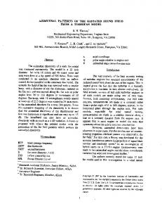
A single combinator generates an overhead of around 7%, and 10 combinators add 50% for the static and 90% for the dynamic approach. In absolute runtime, however, this translates to an overhead of around 17 ms (70 ms) per million nodes and combinator for the static (dynamic) approach. Note that this is a worst-case experiment, since there is no constraint propagation and almost all the time is spent in the combinators. Benchmarks. The second set of experiments shows that in practice, this overhead is dwarfed by the cost of constraint propagation and backtracking. Note that the experiments are not supposed to demonstrate the best possible search heuristics for the given problems, but that a search heuristic implemented using combinators is just as efficient as a native implementation. Fig. 3 compares Gecode’s optimization search engines with branch-and-bound implemented using combinators. On the well-known Golomb Rulers problem, both dynamic combinators and native Gecode are slightly slower than static combinators. 12
Golomb 10 Golomb 11 Golomb 12 Radiotherapy 1 Radiotherapy 2 Radiotherapy 3 Radiotherapy 4 Radiotherapy 5 Job-Shop G2 Job-Shop H5 Job-Shop H3 Job-Shop ABZ1-5 Job-Shop mt10
Compiled 0.61 s 12.72 s 125.40 s 71.13 s 11.78 s 16.44 s 69.89 s 106.04 s 7.25 s 20.88 s 52.02 s 2319 s 2181 s
Interpreted 101.8% 102.9% 100.6% 105.9% 108.3% 107.5% 108.1% 109.2% 146.3% 153.2% 162.5% 103.65% 104.49%
Gecode 102.5% 101.8% 101.9% 107.3% 108.1% 106.9% 98.7% 99.1% 101,16% 107.01% 102.81% 100,13% 99,93%
Fig. 3: Experimental results
On the radiotherapy problem (see Sect. 2.2), the dynamic combinators show an overhead of 6–11%. The native Gecode implementation, which in this case is quite complex, as exh_once is not available in Gecode and must be implemented as a nested search, performs similarly to the dynamic combinators. However, in instances 4 and 5, the compiled combinators lose their advantage over native Gecode. This is due to the processing of exh_once: As soon as it is finished, the combinator approach processes all nodes of the exh_once tree that are still in the search worklist, which are now failed and therefore removed. The native Gecode implementation simply discards the tree. We will investigate how to incorporate this optimization into the combinator approach. The job-shop scheduling examples, using the combination of branch-and-bound and discrepancy limit discussed in Sect. 2.2, show similar behavior. In the two longer running instances, the interpreted combinators show much less overhead than in the shortrunning instances. This is due to a significantly lower number of nodes explored per second (due to more expensive propagation and backtracking), and consequently a reduced overhead of executing the combinators. In summary, the experiments show that the expressivity and flexibility of a rich combinator-based search language can be achieved without any runtime overhead.
6
Related Work
This work directly extends our earlier work on Monadic Constraint Programming (MCP) [13]. MCP introduces stackable search transformers, which are a simple form of search combinators, but only provide a much more limited and low level form of search control. In trying to overcome its limitations we arrived at search combinators. Constraint logic programming languages such as ECLiPSe [4] and SICStus Prolog [16] provide programmable search via the built-in search of the paradigm. User programmable labeling as well as different strategies such as depth bounded, node bounded and limited discrepancy search are available in ECLiPSe. Heuristics cannot 13
be combined arbitrarily, but one can change the strategy, e.g., when the depth bound finishes. Users cannot define their own heuristics or combinators in the library, though they could be programmed from scratch. The Salsa [7] language is an imperative domain-specific language for implementing search algorithms on top of constraint solvers. Its center of focus is a node in the search process. Programmers can write custom “Choice” strategies for generating next nodes from the current one; Salsa provides a regular-expression-like language for combining these Choices into more complex ones. In addition, Salsa allows custom procedures to be run at the exits of each node, i.e., right after visiting it. We believe that Salsa’s Choice construct is orthogonal to our approach, and could be easily incorporated. The custom exit procedures show similarity to our combinator protocol, but no support is provided for arbitrary composition. Oz [17] was the first language to truly separate the definition of the constraint model from the exploration strategy [14]. Computation spaces capture the solver state and the possible choices. Strategies such as DFS, BFS, LDS, Branch and Bound and Best First Search are implemented by a combination of copying and recomputation of computation spaces. The strategies are monolithic, there is no notion of search combinators. The original versions of the constraint modeling language OPL [18,21] provided programmable search using a try construct that creates the search tree. The tree could then be explored with a programmed strategy, or a built-in strategy such as DFS, LDS, BFS or BeFs. Exploration strategies could be modified by limit strategies, which were effectively combinators. Comet [19] features fully programmable search [20], with a clean separation between the specification of the search tree and the exploration strategy. Search trees are specified using the non-deterministic primitives try and tryall, corresponding to our base_search heuristics. Exploration is delegated to a search controller, which, similar to our search combinators, defines what to do when starting or ending a search, failing, or adding a new choice. Choices are represented as continuations rather than the more explicit tree nodes we use. Complex hybrid search heuristics can be constructed as custom search controllers. The main difference to our approach is that search controllers are not composable, but have to be implemented by inheritance (where possible) or from scratch.
7
Conclusion
We have shown how our combinator approach provides a powerful high-level language for modeling complex search heuristics. Its modular implementation relieves system developers from a high implementation cost and yet imposes no runtime penalty. For future work, the next step for us will be a full integration into MiniZinc. Furthermore, parallel search on multi-core hardware fits perfectly in our combinator framework. We have already performed a number of preliminary experiments and will further explore the benefits of search combinators in a parallel setting. We will also explore potential optimizations (such as the short-circuit of exh_once from Sect. 5) and different compilation strategies (e.g., combining the static and dynamic approaches from Sect. 4). Finally, combinators need not necessarily be heuristics that control the search. 14
They may also serve to monitor search, e.g., by gathering statistics or visualizing the search tree. Acknowledgments We thank the reviewers of a previous version of this paper for their constructive criticism. Part of this work was conducted while Tom Schrijvers was visiting National ICT Australia and the University of Melbourne. NICTA is funded by the Australian Government as represented by the Department of Broadband, Communications and the Digital Economy and the Australian Research Council.
References 1. Baatar, D., Boland, N., Brand, S., Stuckey, P.J.: CP and IP approaches to cancer radiotherapy delivery optimization. Constraints 16(2), 173–194 (2011) 2. Cook, W.R.: A denotational semantics of inheritance. Ph.D. thesis, Brown University (1989) 3. Cremet, V., Garillot, F., Lenglet, S., Odersky, M.: A core calculus for Scala type checking. In: Proc. MFCS. LNCS, Springer (Sep 2006) 4. ECLiPSe. http://www.eclipse-clp.org/ (2008) 5. Harvey, W.D., Ginsberg, M.L.: Limited discrepancy search. In: IJCAI. pp. 607–613 (1995) 6. Korf, R.E.: Depth-first iterative-deepening: an optimal admissible tree search. Artif. Intell. 27, 97–109 (1985) 7. Laburthe, F., Caseau, Y.: SALSA: A language for search algorithms. Constraints 7(3), 255– 288 (2002) 8. Marriott, K., Nethercote, N., Rafeh, R., Stuckey, P., Garcia de la Banda, M., Wallace, M.: The design of the Zinc modelling language. Constraints 13(3), 229–267 (2008) 9. Nethercote, N., Stuckey, P.J., Becket, R., Brand, S., Duck, G.J., Tack, G.: MiniZinc: Towards a standard CP modelling language. In: Bessière, C. (ed.) CP. LNCS, vol. 4741, pp. 529–543. Springer (2007) 10. Perron, L.: Search procedures and parallelism in constraint programming. In: Jaffar, J. (ed.) CP. LNCS, vol. 1713, pp. 346–360. Springer (1999) 11. Refalo, P.: Impact-based search strategies for constraint programming. In: Wallace, M. (ed.) CP. LNCS, vol. 3258, pp. 557–571. Springer (2004) 12. Samulowitz, H., Tack, G., Fischer, J., Wallace, M., Stuckey, P.: Towards a lightweight standard search language. In: Pearson, J., Mancini, T. (eds.) Constraint Modeling and Reformulation (ModRef’10) (2010) 13. Schrijvers, T., Stuckey, P.J., Wadler, P.: Monadic constraint programming. Journal of Functional Programming 19(6), 663–697 (2009) 14. Schulte, C.: Programming constraint inference engines. In: Smolka, G. (ed.) CP. LNCS, vol. 1330, pp. 519–533. Springer (1997) 15. Sellmann, M., Kadioglu, S.: Dichotomic search protocols for constrained optimization. In: Stuckey, P.J. (ed.) CP. LNCS, vol. 5202, pp. 251–265. Springer (2008) 16. SICStus Prolog. http://www.sics.se/isl/sicstuswww/site/ (2008) 17. Smolka, G.: The Oz programming model. In: Computer Science Today. LNCS, vol. 1000, pp. 324–343. Springer (1995) 18. Van Hentenryck, P.: The OPL optimization programming language. MIT Press (1999) 19. Van Hentenryck, P., Michel, L.: Constraint-Based Local Search. MIT Press (2005) 20. Van Hentenryck, P., Michel, L.: Nondeterministic control for hybrid search. Constraints 11(4), 353–373 (2006) 21. Van Hentenryck, P., Perron, L., Puget, J.F.: Search and strategies in OPL. ACM TOCL 1(2), 285–315 (2000)
15