spatial relations is the only domain-specific part of our search strategy. ..... combinations and for all 141 products, that are available in all markets. Thus, in total ...
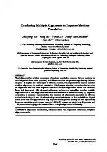
Searching for Objects: Combining Multiple Cues to Object Locations Using a Maximum Entropy Model Dominik Joho Abstract— In this paper, we consider the problem of how background knowledge about usual object arrangements can be utilized by a mobile robot to more efficiently find an object in an unknown environment. We decompose the action selection problem during the search into two parts. First, we compute a belief over the location of the object and subsequently use the belief to select the next target location the robot should visit. For the inference part, we utilize a maximum entropy model which models the conditional distribution over possible locations of the target object given the observations made so far. The model is based on co-occurrences of objects and object attributes in different spatial contexts. The parameters are learned by maximizing the data likelihood using gradient ascent. We evaluate our approach by simulated search runs based on data obtained from different real-world environments. Our results show a significant improvement over a standard search technique which does not employ domain-specific background knowledge.
I. I NTRODUCTION In recent years, the problem of inferring and utilizing semantic information in the context of mobile robot navigation has gained substantial interest [1], [2], [3], [4], [5], [6], [7]. This is motivated by the observation that mobile robots can benefit from semantic information in various ways and that it helps to more efficiently carry out their tasks. Additionally, they allow robots to reason about their environment and can be considered as a major step towards bridging the gap between perception and action. In this paper, we focus on the problem of how background knowledge about the usual arrangements of objects can be utilized to accomplish a search task more efficiently than without such information. The basic idea of our approach is to split the action selection problem during the search process into two parts. First, we compute a belief over possible locations of the target object based on the information about the objects seen so far and the structure of the environment. Second, we utilize the belief to select the next action, e.g., the next position the robot moves to. As an application domain, we consider typical supermarket environments and apply our model to efficiently find the location of a target product in a previously unseen supermarket (see Fig. 1). We have chosen the supermarket scenario as supermarkets are an example of an environment densely populated with many different objects that are arranged in a meaningful way and that exhibit strong spatial dependencies, which can be exploited during the search process. The authors are with the University of Freiburg, Department of Computer Science, Georges-K¨ohler-Allee 79, D-79110 Freiburg, Germany. {joho,burgard}@informatik.uni-freiburg.de
Wolfram Burgard
(a) Supermarket environment.
(b) Searching for a product.
Fig. 1. (a) We model supermarket environments including shelves, products, and a graph. (b) The simulated robot (red square), which does not know the environment, has to search for a product. The search is adapted according to the robot’s belief over the possible product locations, which takes background knowledge about usual object arrangements into account.
The representation for encoding the background knowledge about object arrangements is motivated by the fact that structured indoor environments exhibit meaningful spatial relations between locations that influence the distribution of the objects. For example, one might link two locations by relations like “the same room”, or “the same floor”. Furthermore, we think that in order to be able to generalize from previously seen environments to new environments it is advantageous to represent objects by a list of attributes, instead of thinking of them as atomic entities. For example, even if you have never seen an avocado in a supermarket, it will be useful to know that it is a fruit and it is therefore probably located somewhere where you will see other objects of the category “fruit”. The definition of the object attributes and the types of spatial relations is the only domain-specific part of our search strategy. Accordingly, our approach is therefore generally applicable to different application scenarios, like finding an object in an office environment or a domestic environment as long as it is provided with the corresponding relevant attributes and spatial relations. This paper is organized as follows. After discussing related work, Section III introduces the details of our application scenario. Whereas, Section IV describes maximum entropy models, Section V presents our model to reason about object locations given a partially observed environment. Then, Section VI describes the search strategy that utilizes the inferred belief. Finally, in Section VII, we evaluate this strategy in simulations with data obtained from real-world supermarkets. II. R ELATED W ORK Lau et al. [8] used a computationally involved dynamic programming technique for optimally planning a search path to find multiple stationary targets. Chung and Burdick [9]
Fig. 2. We collected real-world data from four supermarkets, including the market layout, the shelf types, and the products in each shelf. The colors indicate the different shelf types, like normal shelf (yellow), cooling shelf (light blue), freezer (dark blue), or counter (purple).
propose a framework which allows to reason about the possible absence of the target in the search area. Both of these works assume the topology of the environment to be known beforehand. They are able to incorporate prior knowledge in form of a probability distribution over the target location, which is given a priori and then updated based on the detected presence or absence of the target within the robot’s current region. Kollar and Roy [3] presented a technique that allows for estimating such a distribution based on other objects at known locations in a global map. They utilized a Markov random field based on statistics of object co-occurrences and subsequently used the inferred likelihood map to plan a search path. Also previous approaches have addressed probabilistic modeling of object arrangements. Vasudevan and Siegwart [6], for example, modeled different types of places based object counts and inter-object distances and Ranganathan and Dellaert [5] used a 3D constellation model. However, none of these two works address the search problem. Another way to incorporate semantic information into a planning task was presented by Galindo et al. [2]. They defined an ontology about typical domestic environments and then generated plans to find unseen objects or type of rooms, e.g., a bedroom. Cocora et al. [1] investigated the problem of how to efficiently find the entrance hall in a hotel. They learned a relational navigation policy that utilizes the information about the type of rooms and corridors that are directly connected to the robot’s current location. This motivated a previous work of us [10] in which we also considered the shopping scenario. We learned a decision tree that classifies the aisles at junctions into promising and non-promising directions based on the products and product categories that are visible in the corresponding direction. In contrast to many previous approaches, we are searching for an object in an unknown environment and want to be able to utilize the objects seen so far as hints to the location of the target object. Thus, we need to build the map on the fly and generate actions based on partial knowledge about the environment. For this, we rely on background knowledge about usual object arrangements that utilizes a rich set of spatial relations and objects attributes to efficiently guide the search.
product is associated with one of 20 product categories with a coarser granularity like breakfast, dairy products, vegetables & fruits, etc. Further attributes of products are the binary “edible” attribute, as well as the attribute “shelf type”, that denotes in which shelf type the product is usually found in. This can be normal, cooling, freezer, or counter. We consider the basic structural elements of a supermarket to be approximately one meter wide shelves (the small boxes in Fig. 2). Furthermore, we will define a shelf wall unit to be made up of adjacent shelves standing side by side (e.g., the red region marked in Fig. 4). Each shelf contains at least one product and a product might be placed in several shelves. Additionally, the model of a market contains a graph, that constrains the motion of the robot. Each shelf is associated with an access node which is defined to be its nearest graph node. The search process ends, if the robot is located at the access node of a shelf that contains the target product. The robot does not know the environment beforehand but rather has to explore it during the search. The structure of the environment – shelves and graph nodes – can be observed from any distance within the market, as long as they are in the line of sight. In contrast, the products of a shelf can only be detected within a distance of two meters. These visibility constraints are motivated by taking into account the sensor limitations of a real robot. The graph could be extracted from a grid map by using a medial axis transform and the shelf locations could be identified by assuming that each wall in the map is a shelf wall unit. For the actual detection of the objects, we assume that the robot is equipped with an RFID sensor and the products are equipped with RFID tags. In a supermarket environment the robot would then be able to reliably locate a product when it is about two or three meters away. In a previous work, we demonstrated that this is feasible [11]. However, the model described here is not restricted to these sensor modalities, we only require the robot to be able to sense the structure of the environment and to detect and localize objects. The next section will describe maximum entropy models, which we will be using to fuse different spatial cues to the object locations. The subsequent section will then introduce our model for inferring the location of the target object.
III. T HE S UPERMARKET S CENARIO We collected real-world data from four supermarkets, including the market layout and the products in each shelf. We defined a set of 181 products at the granularity of small categories like pizza, apple, shampoo, etc. Additionally, each
IV. M AXIMUM E NTROPY M ODELS In a maximum entropy approach (maxent) [12] a discrete conditional probability distribution P (x | z) is modeled as
x1
follows: �
� exp λ f (x, z) ψ(x, z) � � P (x | z) = P =P ′ T ′ x′ ψ(x , z) x′ exp λ f (x , z) P exp ( k λk fk (x, z)) P =P . ′ x′ exp ( k λk fk (x , z))
neig
T
(1)
hbo
ring
aisl
e
same aisle
neig
g borin
Here, the fk (x, z) are feature functions and the λk are the feature weights, which will be adapted when learning the model. This is the equivalent of a conditional random field with only one node [13], [14]. The log-likelihood of a training set {xi , zi }ni=1 with respect to the set of all feature weights λ is X ℓ(λ) = log P (xi | zi ) (3)
Category (fine)
x2
h
Object1
(2)
aisle
same aisle
Object2 =
Shampoo
Category (fine)
=
Pizza
Category (coarse) = Hygiene
Category (coarse) =
Instant Meal
Edible
=
Edible
=
Yes
Shelf Type
= Normal
Shelf Type
= Freezer
No
Fig. 3. Illustration of the basic idea for inferring object locations based on the detection of object attributes in different spatial contexts. Possible locations of the query object we are searching for are linked to already seen objects by different spatial relations.
i
=
X i
log ψ(xi , zi ) − log
X x′i
ψ(x′i , zi ) .
(4)
The gradient of the log-likelihood with respect to the parameters λ is X X log ψ(xi , zi ) − log ψ(x′i , zi ) (5) ∇ℓ(λ) = ∇ i
=
X i
=
X
x′
Pi
∇ ∇ log ψ(xi , zi ) − P f (xi , zi ) −
i
=
X i
=
X
f (xi , zi ) −
P
x′i
ψ(x′i , zi )
!
(6)
!
(7)
(8)
ψ(x′i , zi )
ψ(x′i , zi )f (x′i , zi ) P ′ x′ ψ(xi , zi )
x′i
X x′i
x′i
i
P (x′i | zi )f (x′i , zi )
(f (xi , zi ) − E [f (xi , zi )]) .
(9)
i
Thus, the gradient is computed as the difference of the empirical feature counts minus their expectation with respect to the model using the current parameters. We additionally use a weak Gaussian prior on the parameters with mean zero and variance 10. To learn the feature weights, we use the RPROP algorithm [15] as an efficient gradient based optimization technique. The optimization problem is convex and the parameters will therefore approach a global optimum. A further useful property of the model is that no independence assumptions between the features have to be made. V. A R ELATIONAL M ODEL FOR I NFERRING O BJECT L OCATIONS We have a set O = {on } of detectable objects and each object is described by a set A = {Ai } of attributes, each with a finite domain D(Ai ) of possible values ai ∈ D(Ai ). We wish to infer the location of a query object oq ∈ O, which we assume to be at one of several possible locations X = {xl }. We furthermore have a set of spatial relations R = {rj }, that relate locations of detected objects to locations x ∈ X, like “same room”, or “same aisle”. We also allow the definition of
overlapping relations, like “same room” and “same house”. The location of a detected object might be linked to several locations xl by different spatial relations rj . See Fig. 3 for an illustration of the basic idea. An observation z in our model corresponds to a tuple z = (xl , rj , Ai , ai ) that states that an object with the attribute Ai = ai has been observed at a location that is related to xl by the spatial relation rj . Thus, a single newly detected object introduces several basic observations zi . By z we denote all observations made so far and z|xl ,rj ,Ai denotes the subset of observation that are constraint to have values xl , rj , and Ai . Throughout the search process, we must update the belief P (x | z) over possible locations x ∈ X of the query object oq that we are searching for, given the observations z made so far. To model P (x | z), we rely on background knowledge about co-occurrences of objects and object attributes in different spatial contexts. This knowledge is expressed by conditional probability distributions P (Ai = ai | oq , rj ) that specify the probability of the following event: given that object oq exists at some location, then there will exist another object with attribute Ai = ai at any location that is related to the location of oq by the spatial relation rj . For example, we might ask that under the assumption that the “coffee cup” that we are searching for is in room x, what would be the probability that we observe a “kitchen object” in “the same room” as room x. Additionally, we need to model P (Ai = ai | ¬oq , rj ) that we will see the attribute in a related location, given the object is not present. To use this background knowledge in form of the abovementioned conditional distributions for computing the desired final distribution P (x | z), we follow a two step process. The idea is to use an ensemble of local models, each considering only a certain aspect of the observations, and then to fuse the local models in a combined model that computes the final distribution. This is motivated by the assumption that the distribution of objects in real-world environments is too complex to be faithfully captured by just a single model and it therefore would be beneficial to combine a diverse set of more simple models. These local models compute the binary probability LAi ,rj (x | z) that the object exists at location x versus that it does not exist at this
(a) Same unit.
(b) Adjacent unit.
(c) Shared path node unit.
(d) Short Euclid. distance unit. (e) Short path distance unit.
Fig. 4. We use five relations between shelf wall units. The reference unit is marked in red (dark gray) and the related units in blue (light gray). The relations are: (a) The same shelf wall unit. (b) Units adjacent to the reference unit. (c) Units sharing a graph node with the reference unit. (d) Units within an Euclidean distance of four meters, or (e) within a path distance of four meters. All relations are reflexive and thus also include the reference unit.
location LAi ,rj (¬x | z). Each local model considers only a certain attribute Ai of those observations z|x,rj ,Ai that are related to x by the relation rj . Now let a(z) denote the set of attribute values that occur in the observations z. Then we model the local models as binary naive Bayes classifiers as follows: LAi ,rj (x | z) Q P (x) z ∈ z|x,r ,A P (z | x) Q j i =P (10) ′ ′ z ∈ z|x,rj ,Ai P (z | x ) x′ ∈{x,¬x} P (x ) Q a ∈ a(z|x,rj ,Ai ) P (Ai = a | oq , rj ) Q . =P ′ o′ ∈{oq ,¬oq } ) P (Ai = a | o , rj ) a ∈ a(z |x,rj ,Ai
(11)
In (11) we dropped the prior P (x), which we assume to be uniform. In total we will have 20 local models as we will be using four attributes and five relations, which we introduce in the next section. The output of all local classifiers LAi ,rj will be used as features fAi ,rj in the maxent model: �P � exp Ai ,rj λAi ,rj fAi ,rj (x, z) �P � . (12) P (x | z) = P ′ x′ exp Ai ,rj λAi ,rj fAi ,rj (x , z)
Thus, the maxent model is used as a way to combine an ensemble of base classifiers. We choose the maxent approach, as it avoids independence assumptions between the features, and thus the local models, which in our case are not independent. Secondly, the model is able to weight the outcomes of the local models by the λAi ,rj and these weights can be learned in a data driven manner. In the experimental section we will also evaluate two other methods for combining the local models. P The first method is a weighted average P (x | z) ∝ i λi Pi (x | z), which is also known as the linear opinion pool. The second Q model isλi the logarithmic which applies opinion pool P (x | z) ∝ i Pi (x | z) exponential weights and corresponds to the geometric mean if the weights are uniform and normalized [16], [17]. There are several possibilities of relating the probabilities LAi ,rj of the local models with the features fAi ,rj of the maxent model. One option is to use the probabilities directly as the features. However, continuous features are usually discretized when used in a maximum entropy approach. Thus, we will also consider to discretize the probabilities in four equally sized bins. Each original feature is then represented
by four binary features, of which only exactly one feature can be non-zero at a time, depending on the probability of the local model. A third option that we consider is to use the log-probability of the local models, in which case the fusion of the local models resembles a logarithmic Q opinion P pool [16], [17], because exp( i λi log(Pi )) = i Piλi .
A. Application to the Supermarket Scenario We wish to infer in which shelf wall unit the target product is located in, given the products seen so far. To apply our model to this scenario, we need to define the object attributes and the spatial relations that we consider to be meaningful in a supermarket. Fig. 4 illustrates the five relations between shelf wall units that we will be using. This includes the relation “same unit”, as well as different types of neighborhood relations, like a unit that shares a graph node with the reference unit, or that is adjacent to the reference unit. Furthermore, we consider relations based on the Euclidean distance and the path distance between shelf wall units. Each relation is reflexive and thus also includes the reference unit. The attributes we are using are the ones depicted in Fig. 3: fine category, coarse category, shelf type, and edible. Examples of the fine and coarse categories that we are using were given in Section III. To learn the feature weights we set up the training data in the following way: first we estimate the conditional probabilities P (Ai = ai | oq , rj ) based on the data of three supermarkets by simply counting the basic events. The local models are then used in the maximum entropy model as features to predict the locations of objects in the remaining fourth supermarket. This is done for all four supermarket combinations and for all 141 products, that are available in all markets. Thus, in total we have 4×141 training examples. We train a single set of parameters. Thus, the learned weights reflect the general importance of each local model when being used to predict a new situation – independent of a specific product or market. During the search process, we will only observe a small fraction of all products in the market. The model is therefore trained on markets in which only some of the shelves contain products. It takes less than two minutes to train the model on a standard PC and each inference during the search takes less than 10 ms. VI. S EARCH S TRATEGIES Once a belief over the target location is computed, the robot needs to decide which action to take next. However,
m shampoo
0
5
10
detection probability > 0.1
0 node utility -0.6
> 0.6
simulated robot
Fig. 5. Example run using the maxent search technique with log-probability features. The position of the robot is marked by the big red square and the path taken is marked by the red line.
we are facing two problems, when planning a path based on the current belief. First, ideally we should take future observations into account, which will change the belief and the subsequent steps. Second, even if we ignore for now that new evidence will change this belief, the problem of planning an optimal search path that minimizes the expected search path length with respect to a given distribution is still NPhard [18], [19]. We will thus settle for a heuristic approach. A. Maximum Utility Node If the robot greedily plans the shortest path to the node with the highest detection probability, it will exhibit undesirable oscillating behavior when there is more than one mode in the belief. We therefore use a strategy that computes a utility U (v) for each node v that trades off the (relative) detection probability P (v) at this node with the (relative) path distance d(v) needed to reach it: U (v) = α ·
P (v) d(v) − (1 − α) · . maxv′ P (v ′ ) maxv′ d(v ′ )
(13)
Selecting a target location by trading off the benefits and costs in a weighted sum has been previously used in autonomous exploration [20], [21]. By adjusting the parameter α ∈ [0, 1] we can alter the search behavior. We tried several parameters in 0.1 increments and found α = 0.4 to result in the shortest paths. The robot moves on the shortest path to the unvisited node with the highest utility until new observations are made and the belief and the node utilities have to be reevaluated. B. Exploration Strategy The exploration strategy serves as a reference strategy, that does not employ domain-specific background knowledge, but instead keeps track of visited and unvisited nodes of the graph. At junctions, it randomly selects among the unvisited successor nodes of the current node. If all successors have been visited already, the robot approaches the nearest unvisited node on the shortest path. If a search technique does not perform better than the exploration strategy, it obviously is not able to utilize domain-specific information, which is the ambition of our strategy. VII. E XPERIMENTAL E VALUATION We search for all 141 products that are available in all four markets. Each product has to be searched for in each of the four markets. When searching in one market, the conditional distributions that capture our background knowledge were
TABLE I OVERALL SEARCH PATH LENGTHS FOR DIFFERENT SEARCH STRATEGIES . Path Length (103 m)
Overhead (to best)
Ratio (to short. path)
shortest path
13.4
−57.6 %
1.0
maxent (log.) maxent (cont.) maxent (discr.)
31.6 32.3 32.5
0% 2.2 % 2.9 %
2.36 2.41 2.43
geom. mean weight. avg.
35.9 36.6
13.6 % 15.8 %
2.68 2.73
geom. mean (mod. 1–3) weight. avg. (mod. 1–3)
38.8 39.4
22.8 % 24.7 %
2.90 2.94
model 3 model 2 model 1
39.9 40.8 51.0
26.3 % 29.1 % 61.4 %
2.98 3.04 3.81
61.3 (σ = 1.4)
94.0 %
4.57
Strategy
exploration
estimated from the remaining three markets. The search starts at the entrance of the market and ends at the node where the product is reachable. When searching for the next product the robot starts again at the entrance without knowledge of the market from the previous run. Different stages of an example search run are depicted in Fig. 5, and the accompanying video illustrates several other search runs. As a performance measure we use the sum of the path lengths of all 4×141 individual search runs. The shortest path from the entrance to a product equals on average about 24 meters. The results are listed in Table I, along with the path length ratio defined as the search path length divided by the shortest path. Additionally, we list the overhead relative to the best search strategy. As the exploration strategy chooses randomly among the directions at junctions, we re-evaluate it ten times and list the mean and standard deviation of the total path lengths. The other strategies are deterministic. We also evaluate the linear and the logarithmic opinion pool with uniform and normalized weights (we will thus refer to them as the weighted average and the geometric mean). Both fusion approaches are also evaluated using either only three local models LAi ,rj or just one model (in this case both fusion approaches are equivalent). These three local models can be considered to be the most specific ones: all use the “Category (fine)” attribute in combination with one of the following spatial relations: “same unit” (model 1), “adjacent unit” (model 2), or “shared path node unit” (model 3). In general, the maxent search strategy achieves the shortest search path which is only about half as long as the one of
Found Products [%]
100 90 80 70 60 50 40 30 20 10 0
world environments. The results showed that our approach is able to reduce the traveled distance by almost 50 % when compared to a standard search technique which does not employ domain-specific background knowledge. ACKNOWLEDGMENT
exploration maxent (log.) weighted avg. geom. mean 1
1.5
2
2.5
3
3.5
4
4.5
5
Search Path Length [ratio]
Fig. 6.
R EFERENCES
Searching for a single product.
Average Path Length [m]
300 250 200 150 100
exploration maxent (log.)
50 1 2 3
5
7
9
11
13
15
17
19
21
Number of Products
Fig. 7.
This work has been supported by the Deutsche Forschungsgemeinschaft (DFG) under contract number SFB/TR 8 Spatial Cognition (R6-[SpaceGuide]).
Searching for multiple products.
the exploration strategy and about 2.4 times longer than the shortest possible path. The usage of different feature representations in the maxent model has only a mild influence on the resulting path lengths. Table I also highlights that the best performance is achieved by strategies that utilize all local models. In Fig. 6 we additionally plot the percentage of found products versus the path length ratio. In Fig. 7 we plot the average path lengths to a product when searching for multiple products. For this, we computed distributions for each of the query products and replaced the detection probability needed for computing the node utilities by the probability of finding any of the query products. The products may be found in any order. As can be seen, employing background knowledge also helps in this situation, though the benefits diminish as the number of objects increase, which is an expected result: the more objects the robot has to find, the more of the search area has to be visited anyway and a exploration strategy might ultimately perform equally well. VIII. C ONCLUSIONS In this paper, we presented a technique that allows a mobile robot to utilize background knowledge about usual object arrangements to more efficiently find an object in an unknown environment. The robot maintains a belief over possible object locations and uses this belief to select its next action. The model is based on co-occurrences of objects and object attributes in different spatial contexts. We used a maximum entropy model to fuse and weight the outcomes of a diverse set of base classifiers that model different aspects of the observations. This was motivated by the assumption that the distribution of objects in realworld environments is too complex to be faithfully captured by just a single model and it therefore would be beneficial to combine a diverse set of simple models. We evaluated our approach by simulated search runs given data from real-
[1] A. Cocora, K. Kersting, C. Plagemann, W. Burgard, and L. De Raedt, “Learning relational navigation policies,” in Proc. of the IEEE/RSJ Int. Conf. on Intelligent Robots and Systems (IROS), Beijing, China, 2006. [2] C. Galindo, J.-A. Fern´andez-Madrigal, J. Gonz´alez, and A. Saffiotti, “Robot task planning using semantic maps,” Robotics and Autonomous Systems, vol. 56, no. 11, pp. 955–966, 2008. [3] T. Kollar and N. Roy, “Utilizing object-object and object-scene context when planning to find things,” in Proc. of the IEEE Int. Conf. on Robotics and Automation (ICRA), Kobe, Japan, 2009, pp. 2168–2173. [4] B. Limketkai, L. Liao, and D. Fox, “Relational object maps for mobile robots,” in Proc. of the Int. Joint Conf. on Artificial Intelligence (IJCAI), 2005, pp. 1471–1476. [5] A. Ranganathan and F. Dellaert, “Semantic modeling of places using objects,” in Proc. of Robotics: Science and Systems (RSS), 2007. [6] S. Vasudevan and R. Siegwart, “Bayesian space conceptualization and place classification for semantic maps in mobile robotics,” Robotics and Autonomous Systems, vol. 56, no. 6, pp. 522–537, 2008. [7] H. Zender, O. Mart´ınez Mozos, P. Jensfelt, G. M. Kruijff, and W. Burgard, “Conceptual spatial representations for indoor mobile robots,” Robotics and Autonomous Systems, vol. 56, no. 6, 2008. [8] H. Lau, S. Huang, and G. Dissanayake, “Optimal search for multiple targets in a built environment,” in Proc. of the IEEE/RSJ Int. Conf. on Intelligent Robots and Systems (IROS), Edmonton, AB, Canada, 2005. [9] T. H. Chung and J. W. Burdick, “A decision-making framework for control strategies in probabilistic search,” in Proc. of the IEEE Int. Conf. on Robotics and Automation (ICRA), Roma, Italy, 2007. [10] D. Joho, M. Senk, and W. Burgard, “Learning wayfinding heuristics based on local information of object maps,” in Proc. of the European Conf. on Mobile Robots (ECMR), Mlini/Dubrovnik, Croatia, 2009. [11] D. Joho, C. Plagemann, and W. Burgard, “Modeling RFID signal strength and tag detection for localization and mapping,” in Proc. of the IEEE Int. Conf. on Robotics and Automation (ICRA), 2009. [12] A. L. Berger, V. J. D. Pietra, and S. A. D. Pietra, “A maximum entropy approach to natural language processing,” Computational Linguistics, vol. 22, no. 1, pp. 39–71, 1996. [13] J. Lafferty, A. McCallum, and F. Pereira, “Conditional random fields: Probabilistic models for segmenting and labeling sequence data,” in Proc. of the Int. Conf. on Machine Learning (ICML), 2001. [14] C. Sutton and A. McCallum, “An introduction to conditional random fields for relational learning,” in Introduction to Statistical Relational Learning, L. Getoor and B. Taskar, Eds. MIT Press, 2006. [15] M. Riedmiller and H. Braun, “A direct adaptive method for faster backpropagation learning: The RPROP algorithm,” in Proc. of the IEEE Int. Conf. on Neural Networks (ICNN), 1993, pp. 586–591. [16] T. Heskes, “Selecting weighting factors in logarithmic opinion pools,” in Advances in Neural Information Processing Systems (NIPS), 1998. [17] A. Smith, T. Cohn, and M. Osborne, “Logarithmic opinion pools for conditional random fields,” in Proc. of the 43rd Annual Meeting of the Assoc. for Computational Linguistics (ACL), 2005, pp. 18–25. [18] K. E. Trummel and J. R. Weisinger, “The complexity of the optimal searcher path problem,” Operations Research, vol. 34, no. 2, 1986. [19] S. J. Benkoski, M. G. Monticino, and J. R. Weisinger, “A survey of the search theory literature,” Naval Research Logistics (NRL), vol. 38, no. 4, pp. 469–494, 1991. [20] A. A. Makarenko, S. B. Williams, F. Bourgault, and H. F. DurrantWhyte, “An experiment in integrated exploration,” in Proc. of the IEEE/RSJ Int. Conf. on Intelligent Robots and Systems (IROS), Lausanne, Switzerland, 2002, pp. 534–539. [21] C. Stachniss, G. Grisetti, and W. Burgard, “Information gain-based exploration using Rao-Blackwellized particle filters,” in Proc. of Robotics: Science and Systems (RSS), Cambridge, MA, USA, 2005.