IIASA International Institute for Applied Systems Analysis • A-2361 Laxenburg • Austria Tel: +43 2236 807 • Fax: +43 2236 71313 • E-mail:
[email protected] • Web: www.iiasa.ac.at
INTERIM REPORT
IR-97-79/October
Searching the Efficient Frontier in Data Envelopment Analysis Pekka Korhonen (
[email protected])
Approved by Gordon MacDonald (
[email protected]) Director, IIASA
Interim Reports on work of the International Institute for Applied Systems Analysis receive only limited review. Views or opinions expressed herein do not necessarily represent those of the Institute, its National Member Organizations, or other organizations supporting the work.
Contents 1. Introduction
1
2. The Multiple Objective Linear Model
2
3. Search of the Efficiency Frontier in DEA
6
4. Numerical Illustrations
8
5. Conclusion
13
References
13
Abstract In this paper, we deal with the problem of searching the efficient frontier in Data Envelopment Analysis (DEA). Our aim is to show that the free search approach developed to make a search on the efficient frontier in multiple objective programming can also be used in DEA. This kind of analysis is needed when among others a) a radial projection is not acceptable, b) there are restrictions on some input and output values, or c) a decision maker (DM) would like to find a decision making unit (DMU) with the most preferred input and output values. The search can be applied to CCR/BCC-models, input-oriented/output-oriented/combined models, and to the models with extra constraints. To make a free search on the efficient frontier, we recommend the use of Pareto Race (Korhonen and Wallenius [1988]) for this purpose. In Pareto Race, the DM may simply control the search with some function keys. The information is displayed to the DM as bar graphs and in numeric form. The search can be terminated at any time, the DM wishes. A numerical example is used to illustrate the approach. Keywords: Data Envelopment Analysis, Multiple Objective Programming, Efficient Frontier, Free Search, Pareto Race
Acknowledgments The research was supported, in part, by grants from the Foundation of the Helsinki School of Economics, the Academy of Finland.
About the Authors Pekka Korhonen is Project Leader of the Decision Analysis and Support Project at IIASA, and also Professor of Economics at the Department of Economics and Management Science, Helsinki School of Economics and Business Administration. More information on the author can be found at the Web site: http://www.iiasa.ac.at/~korhonen
Searching the Efficient Frontier in Data Envelopment Analysis Pekka Korhonen
1. Introduction Data Envelopment Analysis (DEA), originally proposed by Charnes, Cooper and Rhodes [1978 and 1979], has become one of the most widely used methods in operations research/management science. It is easy to agree with Bouyssou [1997] that “DEA can safely be considered as one of the recent "success stories" in OR...” A reason for this success is that DEA is a task-oriented approach and focuses on an important task: to evaluate performance of Decision Making Units (DMU). The analysis is based on the evaluation of relative efficiency of comparable decision making units. Based on information about existing data on the performance of the units, DEA forms an empirical efficient surface. If a DMU lies on the surface, it is referred to as an efficient unit, otherwise inefficient. DEA also provides efficiency scores and reference units for inefficient DMUs. Reference units are hypothetical units on the efficient surface, which can be regarded as target units for inefficient units. A reference unit is traditionally found in DEA by projecting the inefficient DMU radially to the efficient surface. From a managerial point of view, there may be a need sometimes to have some flexibility to choose a reference unit. The reference unit found for an inefficient unit through radial projection dominates the inefficient unit, but it is not the only one on the efficient frontier with that property. This is an important and often desirable property, but why always choose one specific unit. Why not take into account the preferences of the DM? There are several possibilities to incorporate preference information into the analysis, for instance: •
to decide a priori a projection rule or
•
to restrict acceptable input- and output-values, or
•
to assist the DM to make a search on the efficient frontier and let him/her choose the unit which he/she prefers the most.
2
Not many papers have been written on the subject of incorporating preference information into DEA. A few exceptions are Golany [1988], Thanassoulis and Dyson [1992] and Zhu [1996]. A common feature in all these analyses is that first preference information is gathered from the DM, and then this information is used to produce a target unit for an inefficient unit on the efficient frontier. In this paper, our purpose is provide the DM with an interactive method which allows him/her to incorporate preference information into the efficient frontier analysis by enabling him/her to make a free search on the efficient frontier. A requisite technique has already been developed for Multiple Objective Linear Programming (MOLP) models. Because DEA- and MOLP-models are structurally similar, we apply this technique to DEA problems as well. The approach recommended is based on a so-called Reference Direction Approach originally proposed by Korhonen and Laakso [1986]. Korhonen and Wallenius [1988] developed from the original reference direction approach a dynamic version called Pareto Race. Actually, Pareto Race is an interface which makes it possible to move along the efficient surface and freely search various target units in DEA as well. We also demonstrate and discuss various situations in which the approach might be useful in DEA. The rest of this paper is organized as follows. In Section 2 we discuss the use of the reference direction approach for searching the efficient frontier in multiple objective programming. In Section 3 we show how these considerations can be utilized in DEAmodels; Section 4 illustrates the procedure with a numerical example extracted from a real application, and Section 5 concludes the paper.
2. The Multiple Objective Linear Model Assume we have n DMUs each consuming m inputs and producing p outputs. Let X ∈ m× n p× n ℜ and Y ∈ ℜ be the matrices, consisting of nonnegative elements, containing + + the observed input and output measures for the DMUs. We further assume that there are no duplicated units in the data set. We denote by xj (the jth column of X) the vector of inputs consumed by DMUj, and by xij the quantity of input i consumed by DMUj. A T similar notation is used for outputs. Furthermore, we denote 1 = [1, ..., 1] . Consider the following Multiple Objective Linear Program (MOLP): Max
Yλ
Min
Xλ
s.t.
(2.1) n λ ∈ Λ = { λ λ ∈ ℜ+ and Aλ ≤ b},
3
where matrix A ∈ ℜ
k× n
k is of full row rank k and vector b ∈ ℜ .
Model (2.1) - like any multiple criteria model - has no unique solution, in general. Its "reasonable" solutions are called efficient solutions. Definition 1. In (2.1), λ* ∈ Λ is an efficient solution iff there does not exist another λ ∈ Λ such that Yλ ≥ Yλ* and Xλ ≤ Xλ* and (Yλ, Xλ) ≠ (Yλ*, Xλ*) Definition 2. In (2.1), λ* ∈ Λ is weakly efficient iff there does not exist another λ ∈ Λ such that Yλ > Yλ* and Xλ < Xλ*. Specifically, in the MOLP-literature (see, e.g., Steuer [1986]), the concept of efficiency is used to refer to the solutions in the decision variable space ℜn (set Λ) and the concept of dominance is used to refer to the efficient solutions in the criterion space ℜp+m (set T, where T = { (y, x) y = Yλ, x = Xλ, λ ∈ Λ}). A possible and currently popular way to perform the search for solutions on the efficient frontier of a MOLP-problem is to use the achievement (scalarizing) function suggested by Wierzbicki [1980]. Following Wierzbicki, we call the method the Reference Point Method. To characterize the efficient set of problem (2.1), we may use the following formulation: min s(g, u, w,δ ) = min {max [ α i∈P
i
(gi - ui)/wi ] + δ
∑ α i(gi - ui)}
i∈ P
(2.2) s.t.
u = (y, x) ∈ T,
where s is the ASF, w > 0, w ∈ ℜp+m is a vector of weights, α i =1, i=1,…,p and α i = 1, i=p+1,…,p+m, δ > 0 is “Non-Archimedean” (see for more details, Arnold et al. [1997]) and P = {1, 2, ..., m+p}. Vector g ∈ ℜp+m is a given point, the components of which are called aspiration levels. Using (2.2), we may project any given (feasible or infeasible) point g ∈ ℜp+m (called a reference point in MOLP-terminology) onto the set of efficient solutions of (2.1). Varying the vector of aspiration levels, all efficient solutions of (2.1) can be generated (Wierzbicki [1986]). We may also generate efficient solutions by varying the weighting vector w. However, the changes of aspiration levels are easier to handle, because they can be implemented as changes in the rhs-values in a linear programming formulation (see, 2.3a,b).
4
The reference point method is easy to implement. The minimization of the achievement scalarizing function is an LP-problem. In Joro, Korhonen and Wallenius [1995], we have shown that the problem can be written in the following form:
max
Reference Point Model Primal
Reference Point Model Dual
(REFP)
(REFD)
Z =σ +ε (1Ts+ + 1Ts-)
s.t.
min (2.3a)
Yλ -σ w - s = g y
+
y
Xλ +σ wx + s- = gx
λ∈Λ s- , s+ ≥ 0
ε >0
T x T y T W=νg -µg +u b
s.t.
(2.3b) -µ Y + ν X + u A ≥ 0 T T
T
µT wy + νTwx
T
=1
µ, ν ≥ ε 1 u ≥ 0
ε >0
n
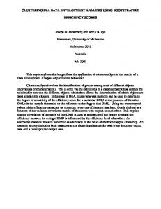
Λ = {λ λ ∈ ℜ+ and Aλ ≤ b} Vector gy consists of aspiration levels for outputs and gx of aspiration levels for inputs y y g w (g= gx). Vectors wy > 0 and wy > 0 (w= wx ) are the weighting vectors for outputs and inputs, respectively. Let’s denote the optimal value of the models Z* and W*. The reference point approach makes it possible to "jump" on the efficient frontier. For y g each given reference point g= gx, the model (2.3a,b) finds a point on the efficient frontier. The reference point approach is a basic technique to project any point (feasible or infeasible) onto the efficient frontier, but to provide a tool for searching the efficient frontier requires further developments of the reference point method. Reflecting on our own bias, we recommend the use of the VIG software to perform the search on the efficient frontier. VIG implements Pareto Race (see, Figure 3), a dynamic and visual free search type of interactive procedure for multiple objective linear programming. It enables a DM to freely search any part of the efficient frontier by controlling the speed and direction of motion. The objective function values are represented in numeric form and as bar graphs on the computer screen. The theoretical foundations of Pareto Race are based on the reference direction approach developed by Korhonen and Laakso [1986]. In the reference direction approach, any direction r specified by the DM is projected onto the efficient frontier:
5
max
σ +ε (1Ts+ + 1Ts-)
s.t.
(2.4) Yλ -σ wy - s+ = gy + try Xλ +σ wx + s- = gx + trx
λ∈Λ s , s+ ≥ 0, -
when t: 0 → ∞. The solution of model (2.4) is an efficient path starting from the current solution and traversing through the efficient frontier until it ends up at some corner point of the efficient frontier as shown in Figure 1. Projection of the Reference Direction A Reference Direction
g
i
q
i+1
Nondominated Set
qi
Feasible Region
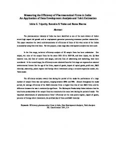
Figure 1. Illustration of the Reference Direction Approach In the original reference direction approach the DM specified a direction, the model generated an efficient path, and the whole path at a time - actually the values of the objective functions on this path – were displayed in a numeric and visual form to the DM as illustrated in Korhonen and Laakso [1986]. Korhonen and Wallenius [1988] developed a dynamic version, which made it possible dynamically and implicitly to vary the reference direction during the process. This approach enables the DM to make a free search on the nondominated frontier. The idea is illustrated in Figure 2.
6
Projection of the Reference Direction A Reference Direction r o
Nondominated Set
q0
Feasible Region
Figure 2: Illustration of the Dynamic Version of the Reference Direction Approach Pareto Race is the implementation of the dynamic version of the reference direction approach as proposed by Korhonen and Wallenius [1988]. In Pareto Race, a reference direction is determined by the system on the basis of preference information received from the DM. By pressing number keys corresponding to the ordinal numbers of the objectives, the DM expresses which objectives he/she would like to improve and how strongly. In this way he/she implicitly specifies a reference direction. Figure 3 provides the Pareto Race interface for the search, embedded in the VIG software (Korhonen and Wallenius [1988]).
3. Search of the Efficiency Frontier in DEA How can we utilize the considerations of Section 2? First, we show how all basic DEAmodels can be introduced from the models (2.3a,b). Let’s consider the primal models. We refer to the unit under consideration by subscript ‘0’. Thus the different models for measuring the efficiency of unit ‘0’ are obtained as shown in Table 1. y g Each model 1-7 produces an efficient solution corresponding to the given g= gx. Models 1-6 performs a so-called radial projection whereas model 7 only consists of a y w radial projection as a special case. Which weighting vector w = wx is used in model 7 determines which efficient solution is obtained. In some problems, it may be reasonable, for instance, to use a constant vector w for all units under consideration. To be precise, we have to notice that the models (1-6) cannot be regarded as special cases of models y w (2.3a,b), because in the reference points model it was assumed w = wx > 0. However, the presence of the term ε (1Ts++ 1Ts-) in the objective function of model (2.3a) according to a classical theorem by Geoffrion [1968] guarantees that all solutions of
7
models are efficient, even if some components wi, i ∈ P, were zeroes. This is a very well known fact also in the DEA-community. Table 1: Modifications of Model (2.3 a) for Different (Primal) DEA-Models #
1
wx
Model Type Output-Oriented CCR-model
gx 0
wy
gy
Λ
0
0
n ℜ+
0
x
y
x0
0
0
y0
n ℜ+
0
x0
y0
0
n {λ λ ∈ ℜ+ and 1Tλ = 1}
x0
0
0
y0
n {λ λ ∈ ℜ+ and 1Tλ = 1}
x0
x0
y0
y0
n ℜ+
x0
x
0
y
-
x0
-
(Charnes et al. [1978])
2
Input-Oriented CCR-model 1)
(Charnes et al. [1978]).
3
Output-Oriented BCC-model (Banker et al. [1984])
4
Input-Oriented BCC-model (Banker et al. [1984]) 1)
5
Combined CCR-model (Joro et al. [1995])
6
Combined BCC-model
0
y
0
(Joro et al. [1995])
7
General Combined model
y0
n {λ λ ∈ ℜ+ and 1Tλ = 1} - 2)
We have now shown above that various CCR- and BCC-models (1-6), and further a general combined model (7), can be presented as a special case of the reference point model. How about efficiency? Is efficiency defined in the same way in MOLP and DEA? Let’s consider how the efficiency is defined in DEA: A DMU is efficient iff Z* = W* = 1 and all slack variables s-, s+ equal zero; otherwise it is inefficient (Charnes et al. 1994). All efficient DMUs lie on the efficient frontier, which is defined as a subset of points of set T satisfying the efficiency condition above. The definition of efficiency and the corresponding definition for weak efficiency, can be given in the following equivalent form: Definition 3. A solution (Yλ*, Xλ*) = (y*, x*) of models 1-7 is efficient iff there does not exist another (y, x) ∈ T such that y ≥ y*, x ≤ x*, and (y, x) ≠ (y*, x*).
1)
x
0
The input oriented models are usually in DEA solved as a minimization problem by writing w =- x and modifying the objective function accordingly. 2)
In this general case, we have to assume that ei ∈ Λ, i =1,…, n, where ei is the i unit vector in ℜ . th
n
8
Definition 4. A point (y*, x*) ∈ T is weakly efficient iff there does not exist another (y, x) ∈ T such that y > y* and x < x*. As we can see Definitions 1 & 2 and Definitions 3 & 4 define efficiency in the same way. The only difference is that in Definitions 1 & 2, the concept efficiency is used in a n variable space (ℜ ) whereas Definitions 3 & 4 defines efficiency in the criterion space (ℜp+m). In spite of a slight terminology difference, the efficient frontier for various DEAmodels can be characterized by an MOLP-model. It means that we may base the efficient frontier search in DEA on accordingly modified model (2.4). If desired, we may restrict the area to be searched on the efficient frontier by setting explicit restrictions to input- and output-values. Traditionally, in DEA the values of input- and output-variables are restricted by setting bounds for the variables of the dual model (2.3b). Which technique is more applicable depends on the problem under consideration.
4. Numerical Illustrations Let’s consider the following numerical example, in which the data in Table 2 are extracted and modified from a real application. Four large super-markets A, B, C, and D are evaluated on four criteria: two outputs (Sales, Profit) and two inputs (Working Hours, Size). "Working Hours" refers to labor force available within a certain period and "Size" is the total area of the super-market. (The super-markets are located in Finland.) Table 2: A Multiple Objective Model A Sales (106 Fim) 6
Profit (10 Fim)
B
C
D
225 79
66
99
5.0
0.2 1.2 1.9 max
Working Hours (103 h) 127 50 3
2
Size (10 m )
8.1
max
48
69
min
2.5 2.3 3.0 min
A managerial problem is to analyze the performance of those super-markets. Initially, a standard DEA is performed by using a CCR-model. (In this example, there is no difference between the CCR-models and BCC-models provided that the null-unit is included in the analysis.) As a result of the analysis, we obtain that markets A, B, and D are efficient and C inefficient. We focus next on the performance analysis of the inefficient unit C. Let’s consider the results of different CCR-models: an outputoriented (model 1), input-oriented (model 2), and combined model (model 5). The solutions of the models are given in Tables 3.a-c.
9
Table 3a: Efficiency Analysis of Unit C with the Output-Oriented CCR-Model (1) A
B
C
D
Max (σ)
Cx
λ-coefficients 0.0709 0.0924 0.0000 0.4981 1.0996
Ref.Unit
Sales
225
79
66
99
-66
72.58
Profit
5
0.2
1.2
1.9
-1.2
1.32
Work Hours
127
50
48
69
48.0
48.00
Size
8.1
2.5
2.3
3
2.3
2.30
Table 3b: Efficiency Analysis of Unit C with the Input-Oriented CCR-Model (2) 3) A
B
C
D
λ-coefficients 0.0645 0.0841 0.0000
Min (σ)
Cy
0.4530 0.9094
Ref.Unit
Sales
225
79
66
99
66.0
66.00
Profit
5
0.2
1.2
1.9
1.2
1.20
Work Hours
127
50
48
69
-48
43.65
Size
8.1
2.5
2.3
3
-2.3
2.09
Table 3c: Efficiency Analysis of Unit C with the Combined CCR-Model (5) A
B
C
D
Max (σ)
C
λ-coefficients 0.0676 0.0881 0.0000 0.4745 0.0475
Ref.Unit
Sales
225
79
66
99
-66 66.0
Profit
5
0.2
1.2
1.9
-1.2
Work Hours
127
50
48
69
Size
8.1
2.5
2.3
3
69.13
1.2
1.26
48 48.0
45.72
2.3
2.3
2.19
Each model will produce a different reference unit on the efficient frontier for C. In the first model, the output values will projected radially onto the frontier subject to the current levels of resources. In the second model the role of the input- and outputvariables have been changed. In the last model, the projection is made by improving the values of the output- and input-variables simultaneously. Of course, the DM may take any of those reference units, or he/she may be willing to consider other possible values 3)
The model is solved as a minimization problem as usually done in DEA
10
as well. If he/she takes, for instance, the input values given, there is still a lot of variation in the output values. The efficient frontier in this problem is trivial - one line. The whole line can be obtained as a convex combination of the output values in columns I and IV in Table 4. In column III, we have the solution on the line resulted by the output-oriented CCR-model in Table 3a. The DM has thus several alternatives to choose the reference unit he/she prefers most. All solutions on the efficient line satisfy the input constraints; they all use the resources less or equal to unit C. (In this example, they use exactly the same amount, but it is not the case in general.) However, all solutions on the efficient line do not dominate the input- and output-values of C. The value of “Profit” in column I is lower than the corresponding value of C. If the DM is interested only in the values dominating those of C, he/she can consider the convex combination of solutions in columns II and IV. As we have seen, the DM has many options to emphasize various aspects in searching for the most preferred unit to C. If for instance "Sales" is important, he/she can choose a solution maximizing "Sales" (solution I in Table 4), but if he/she cannot accept a worse value on “Profit” than on C, the solution in column II might be most preferable. In case, “Profit” is important, the DM might be willing to use as a reference unit the solution in column III. Table 4: Characterizing All Efficient Solutions of the Output-Oriented CCR-Model in Table 3a I Sales
73.61
Profit
0.55
Work Hours
48.00
Size
2.30
A
II
III
IV
72.74 72.58
72.40
1.32
1.45
48.000 48.00
48.00
2.30
2.30
1.20 2.30
0.0599 0.0709 0.0826
B
0.6533 0.1799 0.0924
D
0.2222 0.4551 0.4981 0.5436
The above considerations are very easy to perform if we have only two criteria. The efficient frontier is piecewise linear in two dimensions, and all efficient solutions can always be displayed visually. (The efficient frontier of our example was exceptionally simple.) The characterization of the efficient frontier can also be carried out in a straightforward way e.g. by first identifying all extreme points and then using those points for characterizing all efficient edges. Generally, the efficient frontier cannot be characterized by enumerating all efficient facets by means of the efficient extreme points. Even in quite small size problems, the number of efficient points is huge. Actually, it is not necessary to approach the problem
11
in this way. Even if we could characterize all efficient facets, the DM would need help to evaluate solutions on different facets. Therefore, we recommend a free search on the efficient frontier. Using Pareto Race the DM can freely move on the efficient frontier by controlling the speed and the direction of motion on the frontier as explained in Section 2. Assume that the DM is willing to consider the reference units for C which do not necessarily fulfill the input-constraints. Then the problem becomes four criterion problems, because the DM has preferences over input values as well. Let’s assume the DM will start from the solution in Table 3c, but is not fully satisfied with the solution. He/she may search the neighborhood of the current solution by using Pareto Race (Figure 3) and end up with the solution displayed in Figure 3. Pareto Race enables the DM to search for any part of the efficient frontier.
Pareto Race
Goal 1 (max ): Sales ==> ■■■■■■■■■■■■■■■■■■■■■■■■■■■■■■■■■■■■■■ 69.5465 Goal 2 (max ): Profit ==> ■■■■■■■■■■■■■■■■■■■■■■■■■■■■■■■■■■■■■■ 1.39094 Goal 3 (min ): Working H
==>
■■■■■■■■■■■■■■■■■■■■■■■■■■■■■■■■■■■■ 46.0137 Goal 4 (min ): Size
==>
■■■■■■■■■■■■■■■■■■■■■■■■■■■■■■■■■■■■■■ 2.21314
Bar:Accelerator F1:Gears (B) F3:Fix F5:Brakes
num:Turn
F2:Gears (F) F4:Relax F10:Exit
Figure 3: Searching for the Most Preferred Values for Inputs and Outputs In Pareto Race the DM sees the objective function values on a display in numeric form and as bar graphs, as he/she travels along the efficient frontier. The keyboard controls include an accelerator, gears, brakes, and a steering mechanism. The search on the
12
nondominated frontier is like driving a car. The DM can, e.g., increase/decrease the speed, make a turn and brake at any moment he/she likes. Technically, two parameters are used to control the motion on the nondominated frontier: 1) reference vector r (= direction) and 2) the scalar parameter t (= step size or speed). The mechanism to change those parameters is as follows: • When the DM wants to improve some objectives, change r in such a way that the improvements can be seen in the values of the objectives in question. • When the DM wants to "travel" faster, increase the step-size. To implement those features, Pareto Race uses certain control mechanisms, which are controlled by the following keys: (SPACE) BAR: An “Accelerator” Proceed in the current direction at constant speed. F1: ”Gears (Backward)” Increase speed in the backward direction. F2: ”Gears (Forward)” Increase speed in the forward direction. F3: “Fix” Use the current value of objective i as the worst acceptable value. F4: “Relax” Relax the “bound” determined with key F3. F5: ”Brakes” Reduce speed. F10: “Exit” num: ”Turn” Change the direction of motion by increasing the component of the reference direction corresponding to the goal's ordinal number i ∈ [1, k] pressed by DM.
13
5. Conclusion We have shown that the approaches developed to search the efficient frontier in Multiple Objective Linear Programming (MOLP) are useful in analyzing the efficiency by using Data Envelopment Analysis (DEA). To characterize the efficient frontier of a MOLP-problem, a widely used technique is to transform the problem into a single objective problem by using an achievement scalarizing function as proposed by Wierzbicki [1980]. This transformation leads to a so-called reference point model in which the search on the efficient frontier is controlled by varying the aspiration levels of the values of the objective functions. For each given aspiration level point, the minimization of the achievement scalarizing function produces a point on the efficient frontier. Because the reference point model and models used in DEA are similar, the methods based on the reference point approach can be used in DEA as well. One of those further developments is Pareto Race, a dynamic and visual free search type of interactive procedure for multiple objective linear programming proposed by Korhonen and Wallenius [1988]. The theoretical foundations of Pareto Race are based on the reference direction approach developed by Korhonen and Laakso [1986]. The main idea in the reference direction approach was to parameterize the achievement scalarizing function The search of the efficient frontier in DEA-models is desirable for instance, when the DM would like to have more flexibility in determining a reference unit to an inefficient unit than a radial projection principle provides. Sometimes a DM may be interested to make a search on the efficient frontier just for finding the most preferred unit on the frontier.
References Arnold V., Bardhan, I., Cooper, W.W., Gallegos, A. (1997), “Primal and Dual Optimality in Computer Codes Using Two-Stage Solution Procedures in DEA”, (Forthcoming in Aronson, J. and S. Zionts (Eds.): Operations Research: Models, Methods and Applications, Kluwer, Norwell. (A Volume in honor of G.L. Thompson)). Banker, R.D., Charnes, A. and Cooper, W.W. (1984), “Some Models for Estimating Technical and Scale Inefficiencies in Data Envelopment Analysis”, Management Science 30, 1078-1092. Bouyssou, D. (1997), "DEA as a Tool for MCDM: Some Remarks", (The paper was presented at the Fifth European Workshop on Efficiency and Productivity Analysis, Copenhagen, October 9-11, 1997) Charnes, A., Cooper, W., Lewin, A.Y. and Seiford, L.M. (1994) Data Envelopment Analysis: Theory, Methodology and Applications, Kluwer Academic Publishers, Norwell.
14
Charnes, A., Cooper, W.W. and Rhodes, E. (1978), “Measuring Efficiency of Decision Making Units”, European Journal of Operational Research 2, 429-444. Charnes, A., Cooper, W.W. and Rhodes, E. (1979), “Short Communication: Measuring Efficiency of Decision Making Units”, European J. Operational Res. 3, 339.
Geoffrion, A. (1968), "Proper Efficiency and the Theory of Vector Maximisation", Journal of Mathematical Analysis and Applications 22, pp. 618-630. Golany, B. (1988), “An Interactive MOLP Procedure for the Extension of DEA to Effectiveness Analysis”, Journal of Operational Research Society 39, 725-734. Joro, T., Korhonen, P. and Wallenius, J. (1995): "Structural Comparison of Data Envelopment Analysis and Multiple Objective Linear Programming", (Forthcoming in Management Science), (Working Papers W-144, Helsinki School of Economics). Korhonen, P., and Laakso, J. (1986). "A Visual Interactive Method for Solving the Multiple Criteria Problem", European Journal of Operational Research 24, pp. 277287. Korhonen, P. and Wallenius, J. (1988), "A Pareto Race", Naval Research Logistics 35, 615-623. Steuer, R.E. (1986), Multiple Criteria Optimization: Theory, Computation, and Application, Wiley, New York. Thanassoulis E. and Dyson R.G. (1992), “Estimating Preferred Target Input-Output Levels Using Data Envelopment Analysis”, European Journal of Operational Research 56, 80-97. Wierzbicki, A. (1980), “The Use of Reference Objectives in Multiobjective Optimization”, in G. Fandel and T. Gal (Eds.), Multiple Objective Decision Making, Theory and Application, Springer-Verlag, New York. Wierzbicki, A. (1986), “On the Completeness and Constructiveness of Parametric Characterizations to Vector Optimization Problems”, OR Spektrum 8, 73-87. Zhu, J. (1996), “Data Envelopment Analysis with Preference Structure”, Journal of the Operational Research Society 47, 136-150.
15