SEASONAL VARIATIONS IN YIELD FOR DIFFERENT TYPES OF PV MODULES MEASURED UNDER REAL LIFE CONDITIONS IN NORTHERN EUROPE O.M. Midtgård and T.O. Sætre Agder University College, Faculty of Engineering and Science, Grooseveien 36, NO-4876 Grimstad, Norway email:
[email protected],
[email protected] ABSTRACT: A test setup which enables the automatic and continuous retrieval of I-V characteristics for PV modules is presented. The setup is custom made from relatively inexpensive equipment. Results that compare performance in 2004 and 2005 are presented, and show crystalline modules to be preferable from the point of view of efficiency. Further results show the seasonal variations in yield over the whole of 2005. Based on the results, we conclude that photovoltaic technology is a viable alternative even in a cold and periodically dark country like Norway. Keywords: PV Module, Performance, Experimental Methods 1
INTRODUCTION
The purpose of the work presented in this paper is to study and compare the performance of various types of commercially available PV modules (monocrystalline, multicrystalline and amorphous) under real life conditions in Northern Europe. Previously, results from the summer of 2004 have been reported [1]. In that paper, the emphasis was on studying the variations in the Fill Factors and other main data of the modules. In the present paper, results for both warm and cold seasons in 2005 are reported, as well as a comparison between 2004 and 2005. In addition, further details about the experimental setup are explained, complementing what has already been described in [1]. 2
seven boxes that correspond to the outdoor equipment is shown: the three PV modules, as well as a sensor for the ambient temperature and a pyranometer. Each of the modules is connected to its own electric load, which is controlled via a LabView programme and National Instruments’ NI CB 6.8LP I/O card. Moreover, all measured quantities are fed to the LabView programme via the same card, and then stored on a computer. The pyranometer used is a SolData 80SPC, which is a global insolation sensor. This sensor is fixed on the frame of the amorphous module, and can be spotted in Fig. 1.
METHOD
2.1 Modules being tested Various commercially available PV modules – shown in Fig. 1 – are continuously monitored in the town of Grimstad, in Southern Norway.
Figure 1: PV modules being monitored in Grimstad. Here, we present results from and compare three of these modules – an amorphous, a monocrystalline and a multicrystalline module. These are, respectively, the US64, the GPV110M, and the GPV51W, and they are the three modules seen from the left in Fig. 1. (The other two modules correspond to a setup where the effect of using a reflector is investigated; this is not reported here.) 2.2 Main components of the data acquisition system An overview of the test setup system is shown in Fig. 2. The system is built in-house from relatively inexpensive equipment. In the upper part of the figure
Figure 2: Overview of the test setup and its main components. 2.3 Description of electric loads A very important part of the setup is the custommade electric loads. The data for a PV module is retrieved by tracing its I-V curve. For this purpose, an electronically controlled variable resistance must be connected to the PV module’s terminals. Ideally, the resistance should be variable from infinite (open circuit) to zero (short circuit). A MOSFET-transistor is a voltage controlled variable resistance. However, its drain-source resistance is a very non-linear function of the applied gate-source voltage VGS, and it may therefore be recommendable to use some
additional components to have better control over its behavior. Fig. 3 shows an ideal circuit that in principle can be used to control current flow. The applied voltage VSET at the non-inverting terminal of the (ideal) operational amplifier (op-amp) is also present at the inverting terminal, due to the infinite (very large) amplification of the op-amp. Thus, this voltage is also present over the measuring resistance RM, and the current I flowing through RM, and the MOSFET-transistor, is equal to VSET/RM. (The gate-voltage of the MOSFETtransistor is adjusted by this feedback-system such that this behavior is achieved.)
Figure 3: Principle for electric load.
data are retrieved, most importantly the currents and voltages for the PV modules. In the GUI, the user of the system can configure the start-time, the stop-time and the interval between measurements. In the present case, with only a few exceptions over the year reported (2005), the start-time was set to 08:00 and the stop time to 20:00, with an interval between measurements of 20 minutes. The data are stored in files, one file for each day. In addition the user can choose to make manual measurements without stopping the main flow of the program, and individual IV curves can be stored. The GUI is depicted in Fig. 5. Details are not clearly visible, but the screen shot gives a certain impression of what the system looks like. Five IV curves can be seen – one for each PV module depicted in Fig. 1. These curves correspond to the last measurements. In addition, the screen shows the main data retrieved for this measurement. A visual check on whether the system operates properly is therefore at all times available.
However, in practice, several MOSFET-transistors must be connected in parallel due to the relatively large power of the PV modules, and due to the on-state resistance of the MOSFETs. Practice showed that the configuration shown in Fig. 3 then became oscillatory, and therefore a modification of the basic principle was devised and implemented. The resulting configuration is shown in Fig. 4.
Figure 4: Modification of the basic principle to eliminate unstable behavior when paralleling several circuits. Now, the op-amp is connected as a summation amplifier, and a negative set-point voltage VSET is therefore applied in order to amplify the difference between the two voltages. It is easy to find an expression for the current I as a function of the voltages VSET and VGS, but virtually impossible to find a closed expression that eliminates VGS from the equation in favor of I. However, we can look at the circuit from a control engineering perspective: There is a (complicated and non-linear) transfer characteristic between VGS and I. The voltage over RM is proportional to I (=RMI) and in the summation amplifier, the difference between the set point voltage (which is now actually a reference current) and RMI is amplified by the factor R2/R1. This amplified voltage is precisely VGS, and we have thus made a feedback control system for the current through the PV module. A block diagram showing the circuit from this perspective can be found in [1]. 2.4 Software and GUI The electric loads are controlled with a LabView programme via the low cost NI CB 6.8LP I/O card. The I-V curves of all modules are traced at periodic intervals by decreasing the reference current from a high value to zero in small steps. At the same time all measurement
Figure 5: The graphical user interface for the software that controls the system. 3
COMPARISON BETWEEN 2004 AND 2005
In a previous paper, we compared measurements that were obtained during the period 29 June - 15 August 2004 to performance data given in the data sheets of the PV modules [1]. Below, data for the same period in 2005 are compared to the results of 2004. 3.1 Main data Manufacturers of PV modules typically report power, current and voltage at the maximum power point (MPP), as well as short circuit current, open circuit voltage, Fill Factor and efficiency measured under STC, i.e. 1000 W/m2 @ 25 ºC cell temperature and AM1.5. The modules that are monitored in the present work are placed in a real life environment, and the conditions cannot be controlled in the same manner. Therefore, the following procedure has been used to recreate similar data for our setup: All recordings for the period in question where the global radiation is measured to more than 800 W/m2 are collected. For these levels of radiation a graphic analysis shows that the measured quantities have a good regularity, although with a certain spread, especially for the open circuit voltage. The data corresponding to these measurements are then linearly
Multicryst GPV51
Amorphous US-64
PMPP [W] Data sheet 110 51 64 2004 93 43 87 (*) 2005 92 42 51 IMPP [A] Data sheet 6.3 3.0 3.88 2004 6.1 2.8 5.8 (*) 2005 6.0 2.7 3.5 VMPP [V] Data sheet 17.5 17.0 16.5 2004 15.2 15.4 15.0 2005 15.3 15.5 14.4 ISC [A] Data sheet 7.28 3.2 4.8 2004 6.9 3.0 7.3 (*) 2005 6.8 3.0 4.5 VOC [V] Data sheet 21.36 21.5 23.8 2004 19.4 19.6 20.7 2005 19.7 19.8 20.7 FF Data sheet 0.71 0.74 0.56 2004 0.69 0.72 0.58 2005 0.69 0.71 0.55 η [%] Data sheet 14.4 14.2 6.8 2004 12.2 11.9 9.3 (*) 2005 12.1 11.8 5.4 Table_I: Comparison of given and measured performance. Unexpected values, probably caused by faulty measurements, are indicated with an (*). For the given period in 2004 there were 1513 recordings. Slightly more than 20% of these corresponded to measured radiation of greater than 800 W/m2. For the same period in 2005, we had 1501 good recordings, and about 15% of these were in the category of radiation above 800 W/m2. The main data for the two years were calculated according to the procedure given above, and the results are given in Table I. The data for 2005 and 2004 are remarkably similar for the two crystalline modules. This indicates that little degradation of these modules has taken place during the year in between, at least for the radiation-levels concerned. It should be pointed out that no effort has been made to clean the modules. In the summer periods they typically have had a yellowish layer of dust on them – i.e pollen etc., and in the wintertime they have been subjected to harsh conditions such as freezing temperatures and snow. The data for the amorphous module (US-64) is less reliable. In a previous paper [1] we indicated that the higher than expected performance data for 2004 could be caused by a calibration problem of the data acquisition system, but we also speculated whether the data was understated by the manufacturer,
0.1 Efficiency
Monocryst GPV110
backed up by other published tests [2] and statements made by the manufacturer [3]. However, in the mean time the setup has been disassembled, and reassembled, and we now strongly suspect the current measurement of the amorphous module to have been inaccurate previously, although the exact nature of the erroneous measurement has not been identified. But it seems that the current has been erroneously scaled with a constant factor. Assuming this to be the case, it should be noted that these faulty measurements do not influence on any other values than the currents themselves and the efficiency. The results for 2005 look much more in line with what should be expected, and it may seem that the amorphous module has an energy yield per square meter of only about 45 % compared to the crystalline modules under the best conditions.
0.05 monocrystalline 0 0
200
400
600
800
1000
1200
Radiation [W /m 2]
0.1 Efficiency
regressed using least squares and the fitted curves are evaluated at 1000 W/m2. Although the data thus generated do not correspond to STC, it still allows for a rough comparison with the given data. Besides, the procedure allows us to compare data for various time periods in a consistent manner.
0.05 monocrystalline 0 0
200
400
600
800
1000
1200
Radiation [W/m2]
Figure_6: Efficiency versus measured global radiation for the monocrystalline module. Top graph: summer 2005. Below: summer 2004. (1 corresponds to 100%) 3.2 Qualitative comparison We have also qualitatively compared the results over the whole spectrum of radiation, by plotting all the main data versus radiation. A representative example is shown in Fig. 6, where efficiency versus radiation is plotted for both years for the monocrystalline module. It appears as if the spread in values is larger in 2005 compared to 2006, but we would not draw any conclusions based on this alone, since we cannot know whether the effect is caused by the modules, the weather or the experimental setup itself. A comparison of the Fill Factors for the tested modules was reported in [1]. The amorphous module showed good stability in this respect even at low radiation, whereas the crystalline modules had significant deviations. The new measurement series confirms this.
4
SEASONAL VARIATIONS IN YIELD
For the year 2005, we have collected data in every month of the year, although some of the months with incomplete data sets. The total energy yield per month per module has been estimated based on these measurements. The estimated values are based only on the measurements logged during the month, assuming that these data are representative for the month. This is, of course, a questionable approach. To evaluate the actual expected values, continuous measurements over several years must be performed, or more sophisticated statistical analyses of the data must be carried out, correlated with general weather data. However, the simple approach chosen here gives us a snapshot of the situation for the year in question. 4.1 Description of the procedure The measured global radiation is integrated over the day (constant radiation over the interval is assumed until the next measurement) from 08:00 until 20:20 hrs. (The last measurement takes place at 20:00 and the time interval is 20 minutes.) This gives the available energy from the sun over the day. All days with measurements for the chosen month are summed. The average value is thereafter calculated and multiplied with the number of days. This is the estimated energy yield from the sun for the month in question. For a PV module, a similar procedure is followed. However, small radiation levels are more difficult to utilize than higher, and considering that there will be losses also in auxiliary equipment, we disregard all measured radiation levels of less than 150 W/m2. In other words, for radiation levels less than this, the produced power of the module is set to zero, even if we have recorded non-zero values. The energy yield for all modules is thereafter normalized to give values per square meter. This is expressed also in Eq. (1). M N
∑∑ P≥150 (t i ) ⋅ ∆t Em =
j=1 i =1
M ⋅ A PV
⋅ D m [J /m 2 ]
(1)
Em is the energy per square meter for a month, M is the number of measured days for the month, N is the number of measuring points for the day, APV is the area of the module, and Dm is the number of days in the month. Note that for the calculation of the solar energy, all radiation levels were included, whereas for the modules produced power was set to zero when the radiation from the sun was less than 150 W/m2, indicated by the symbol P≥150. 4.2 Estimated energy yield per month for 2005 The results from these calculations are presented in Table II. For this year, the potential from the sun seems to have been about 1063 kWh/m2, as seen in the row denoted Total. The overall efficiencies over the year for all modules are shown in the last row; again we can see the much lower performance of the amorphous module than the two crystalline. As could be expected, the darkest winter months, November-February, give the least amount of energy, but some production takes place even in this period. Surprisingly, perhaps, for this particular year, April seems to have been the best month. The estimated total energy available from the sun over the year fits well with
the expected value for Southern Norway, and the overall efficiencies also indicate that the measurements are reasonable. Based on these numbers using the gross efficiency of the monocrystalline module, about 49 square kilometers of Southern Norway would have to be covered with solar cells to supply Norway’s present total consumption of electric energy per year (about 120 TWh). For this calculation we have assumed 90% electrical efficiency, and that 1 m2 of solar cells requires 2 m2 of land area [4]. Estimated energy yield [kWh/m2] Sun Mono Multi Am Jan 52.3 5.26 5.31 2.04 Feb 42.3 5.50 4.69 1.84 March 111.0 14.0 12.59 5.39 April 149.8 15.19 17.40 7.59 May 126.7 13.12 13.59 6.21 June 132.1 13.66 13.23 6.09 July 134.6 13.84 13.76 6.39 Aug 120.4 12.69 12.09 5.46 Sept 107.3 11.17 10.56 4.47 Oct 66.0 7.41 7.23 3.17 Nov 8.49 0.46 0.37 0.098 Dec 12.0 0.81 0.71 0.29 Total 1063 113 111.5 49 10.6 10.5 4.6 η [%] Table_II: Estimated seasonal variations in yield (snapshot of the actual situation for the measured days of 2005). # days refers to the number of days with measurements for the month. The “Sun” column refers to measurements by the pyranometer. Month
5
# days (M) 12 28 20 30 31 30 27 31 30 14 9 20 282
CONCLUSIONS
We have presented measurements on commercially available PV modules, and given more details on the setup used – a setup that is made in-house, is relatively inexpensive, and has some original features. The results presented shows that the crystalline modules perform much better than the amorphous module tested. Certainly, other arguments than energy yield must be used for the employment of amorphous technology. In our opinion, the gross numbers taken over the whole year of 2005 clearly shows that photovoltaic technology is a viable alternative also in a cold and periodically dark country like Norway. REFERENCES [1] O.M Midtgård, N. Andersson, T.O. Sætre, “Comparison of fill factor for three different types of PV-modules under changing weather conditions,” Proceedings 20th European Photovoltaic Solar Energy Conference, 2005, pp. 2147-2150. [2] http://members.optusnet.com.au/~doranje/Tests.html, “Independent Performance Tests.” [3] Uni-Solar, “Framed Solar Modules, US-Series,” manufacturer’s data sheet, 2004. [4] J.A. Turner, “A realizable renewable energy future,” Science, vol. 285, 30 July 1999, pp. 687-689.