Seasonal Wireless Sensor Network Link Performance in ... - IEEE Xplore

2014 Eleventh Annual IEEE International Conference on Sensing, Communication, and Networking (SECON)

Seasonal Wireless Sensor Network Link Performance in Boreal Forest Phenology Monitoring C.J. Rankine & G.A. Sanchez-Azofeifa

Mike H. MacGregor

Dept. Earth and Atmospheric Sciences University of Alberta Edmonton, Canada [email protected], [email protected]

Dept. Computing Sciences University of Alberta Edmonton, Canada [email protected] Canadian boreal [2], more than 25 years’ worth of current global greenhouse gas emissions. As the climate in northern latitudes changes there have been detectable shifts in growing season lengths [3] with little certainty in how these shifts in plant phenology influence net ecosystem exchange and carbon balances in the vast boreal forests. Like all plant communities, the primary productivity of northern ecosystems is strongly regulated by weather conditions. Meteorological and micro-meteorological dynamics can be challenging to observe in remote locations due to accessibility, power, and communication limitations. While global remote sensing systems provide us with meteorological and forest productivity information these data come at coarse spatial and temporal resolution. For high temporal resolution of boreal forest micro-meteorological variables and remote sensing ecosystem productivity validation we employ wireless sensor networks (WSNs) for distributed area monitoring of canopy-absorbed photo-synthetically active radiation (APAR), air temperature, relative humidity, soil moisture, and the normalized difference vegetation index (NDVI) based on dual broadband light sensors. Boreal forest ecosystems present challenging radio environments for the implementation (design and operation) of wireless sensor networks. In this environment, radio signal excess path loss is difficult to predict due to the complexity and seasonal dynamics of canopy structure, woody area, and weather conditions. These factors also make the long-term network performance uncertain. Here we report on one year of operation of a 2.4GHz wireless network (802.15.4) in a Canadian boreal forest setting, and examine the relationship between several logged network and environmental metrics:

Abstract— While indoor wireless sensor network (WSN) research has recently flourished for monitoring civil and industrial infrastructure, considerably less attention has been given to the development of reliable outdoor WSNs capable of long-term operation in challenging remote locations. We present wireless sensor network link performance results from the first year of monitoring micro-meteorological conditions alongside the 802.15.4 link received signal strength indicator (RSSI) within an old growth stand of deciduous boreal Aspen forest (Populus tremuloides) in Northern Alberta, Canada. Thirty-six weather proof nodes were equipped with meteorological sensors and distributed across one hectare in the forest understory to assess the application of WSNs for observing high resolution changes in seasonal ecosystem productivity and forest phenology. We describe here the density distribution of node RSSI using Gaussian kernel density estimates in relation to node antennareceiver orientation and vegetation seasonality. RSSI across the network displays a lognormal distribution with an increasing bimodal tendency with path length through the forest stand. Spatial variability in RSSI is discussed with respect to forest structure. A strong temporal relationship between RSSI variability and plant canopy development is observed with a 20dBm or 100 fold difference in mean network radio signal power from spring leaf presence to fall leaf absence. The meteorological and biophysical factors associated with this trend are explored using multiple regression and relative factor importance analysis. Our results indicate that in addition to meteorological data, spectral vegetation density metrics are useful in assisting deployment planning and network performance diagnostics when using wireless sensor networks for remote forestry applications. The longevity and performance of this outdoor WSN can be seen as a new standard for harsh network-climate tolerance in northern boreal environments. Keywords— Wireless Sensor Networks, Forests, RSSI, Micrometeorology, Phenology.

 802.15.4 link received signal strength indicator (RSSI) and node-receiver spatial orientation

I. INTRODUCTION

 Temporal variations in RSSI with seasonal evolution of forest canopy biophysical structure as a function of phenology

Carbon sequestration, water storage and purification, and biodiversity tend to be greatest in forested landscapes due to higher primary productivity rates and habitat diversity [1]. As such we associate a higher ecosystem service value for forests than other terrestrial land cover classes [1]. The Canadian boreal forest is the largest biome in North America covering nearly six million km2 and 58% of Canada’s land area [2]. An estimated 208 billion metric tonnes of carbon are stored in the

 Temporal variations in RSSI with daily mean air temperature, vapor pressure, solar insolation, and wind speed during different growth phases of the forest.

978-1-4799-4657-0/14/$31.00 ©2014 Crown 978-1-4799-4657-0/14/$31.00 ©2014 IEEE

302


been the traditional testing grounds for long-term real-time wireless sensor networks. Our study moves to the real testing grounds of an extremely remote setting where access is restricted for 4-6 months of the year during the winter and the old growth forest retains undisturbed natural features.

II. RELATED WORK A.

Radio Propagation Through Vegetation

Radio signal attenuation is unavoidable due to free-space path loss, and is further mediated by signal reflection, refraction, diffraction, and absorption during wave propagation. Besides the fixed parameters of antenna-receiver specifications radio frequency (RF) transmissions in outdoor settings are influenced by local topography, terrain contours, weather, and the properties of path interception materials. The effects of vegetation on RF propagation have been widely investigated for telecommunications but not as extensively for ad hoc wireless sensor networks [4][5]. Typical empirical studies measure excess path loss beyond what is expected given transmitter-receiver parameters to indicate vegetation signal fade [4][6]. Attenuation due to vegetative loss has been demonstrated for frequencies between 30MHz and 60Ghz, with evidence of more pronounced fade at frequencies above 1GHz as wavelengths become smaller than plant structures [ 4]. Depending on canopy height and antenna-receiver orientation there is potential for several main signal transmission routes including ground reflection, surface-wave propagation over the top of plant canopies, and through scatter/diffraction around leaves, branches and tree trunks [4][ 6]. Modelling this path loss generically has proved difficult due to the diversity of vegetation architecture. Forests structure can be particularly complex having varying contributions of foliar and woody densities paired with the heterogeneous distributions of vertical and horizontal forest strata.

C.

The effects of weather conditions on wireless communications have garnered the attention of radio physicists and cellular communication companies since the mid-20th century. Such studies report that only high temperatures (>25°C) cause significant degradation of radio signals [4]. This temperature dependent signal quality was recently described for an outdoor deployed WSN by [17]. Although the cause of this temperature dependent behavior in is unclear it is often considered to be due to antenna mechanics or electronic hardware limitations at higher temperatures [18]. Precipitation does tend to produce intermittent signal fading as well but these are typically short-term interference events and are more pronounced at higher frequencies [6][19]. Interestingly the influence of water vapor on 2.4 GHz sensor network communication is still not well understood; some reports indicate no effect of humidity levels while others have observed minor correlations [10][11]. It is likely that these mixed results originate from the diversity of methods used to measure such a response [17]. For our purposes, as discussed in [17], we do not use relative humidity but rather water vapor pressure as a metric for RSSI-humidity comparisons. Finally, wind movement through vegetation has been observed to increase the variance of received radio signal strength due to the changes in multi-path propagation as trees sway in the wind. [20] and [21] showed that high wind speeds produced radio signal fading of 1.8GHz through 60GHz radio frequencies due to stochastic Rician interference.

Network RSSI: While WSNs are not typically equipped with network analyzers to measure radio frequency response or absolute power both 802.11 and 802.15.4 RF physical layers do provide received signal strength (RSSI). This can be converted to a signal power indicator in dBm through network specific parameters; however this means that there is no standardized RSSI metric used in WSNs. Although RSSI is a useful network communication diagnostic tool it has not been demonstrated as an accurate predictor of absolute node distance or position in a WSN [7][8]. B.

Outdoor Wireless and Weather

Motivation: We are not aware of any other examples of WSNs being applied to forest phenology monitoring nor has there been any demonstration of stable long-term operation of WSNs in remote old-growth forest settings. We believe this is the first study to explore the use of WSNs in vegetation that quantifies the effect of plant canopy development and senescence on radio network communication.

WSNs in Forest Applications

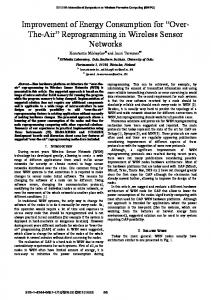
While there has been a significant increase in wireless sensor network research in the last few years, the majority of studies deal with simulated networks [9]. An increasing number of applied outdoor WSNs are being studied but very few of these deployments can be considered long-term and typically report testing operations on the scale of days to weeks [10][11][12]. Uses for WSNs in forest monitoring are plentiful and have been observed already for forest fire detection [13], stream flow [14], snow and soil moisture [15], and microclimate monitoring [16]. To our knowledge no other WSN system exists for tracking forest phenology and none of the reported networks operate far from an urban center. Due to the ease of human access, reliable power source, and network gateway connectivity, urban forest and parkland settings have Fig. 1. WSN Study plot is located in north-western Alberta, Canada in an old growth stand of deciduous boreal forest.

This study was made possible by the National Science and Engineering Council of Canada (NSERC), the Government of Alberta, IBM Smarter Planet, and the Canadian Foundation for Innovation.

303


III.

EXPERIMENTAL OVERVIEW

While the implementation of this remote wireless sensor network was primarily motivated by investigation of boreal forest primary productivity, phenology, micro-meteorological monitoring, and remote sensing validation, this analysis of network performance is essential for continued progress in optimized planning of forest WSN deployments. A. Study Site The monitoring instrumentation is located within the joint industry-research forestry district for Ecosystem Management Emulating Natural Disturbance (EMEND) for large-scale variable retention boreal forest harvest experimentation in northwestern Alberta, Canada (Fig. 1). Regional climate is characterized as humid continental. Mean annual temperature of the nearest long-term weather station 85km SE is 1.2°C (min/max recorded extremes = -49/37°C) with a mean annual precipitation of 400mm and mean snow depth of 12cm [22]. The study plot, located at 56.74 lat. -118.35 long and 870m elevation, is situated in an old-growth stand of Trembling Aspen (Populus tremuloides) with a broad leaf deciduous canopy (Fig.1). There are two generally distinct vertical layers of vegetation, the understory from the ground up to 4m height and the overstory canopy at 15-20m with an observed decreasing woody density with height. A 30m tall carbon flux tower was constructed just outside the forest in a clearing and used as the base station for centralized data aggregation. Our monitoring initiative began in mid-summer of 2012 and is ongoing. B.

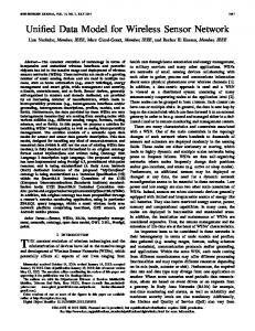
Fig. 3. Wireless environmental monitoring sensor node for forest micro-meteorology and phenology. Radiated power is programmable from 0 dBm (1 mW) to 20 dBm (100mW) for extended range communication with a bidirectional RF link using IEEE 802.15.4 data packet delivery architecture. Nodes use a 2.5 dBi gain omnidirectional antenna with linear polarization. Circuitry is encased in weather proof, pressure dynamic enclosures rated at IP X7. Received signal strength indicator (RSSI) is reported in dBm with a max RSSI around -20dBm and complete data packet loss below -90dbm. Thirty-six nodes were mounted at 1m height in a hexagonal or honeycomb topology (20m sides) over a plot of roughly one ha of forest adjacent to the instrumentation tower (Fig. 2). Nodes were positioned with their antennas vertical and on the receiver side of the post to minimize interference (Fig.3). Each node has a digital temperature and relative humidity sensor placed in a solar radiation shield and upward facing hemispherical photo-synthetically active radiation (PAR) sensor (Apogee SQ-110). Several nodes were further instrumented with soil moisture probes measuring volumetric water content. Tower nodes were equipped with both PAR sensors and pyranometers (Apogee SP-110) for monitoring above canopy incident and reflected radiation for determining the broadband NDVI [24]. The entire network samples with sub-second clock synchronization and was configured for five minute sampling during the growing season and thirty minute sampling for the winter.

Sensor Network Deployment

Our wireless sensor system was co-developed at the University of Alberta’s Center for Earth Observation Sciences via Hoskin’s Scientific and Lord-Microstrain Sensing Systems partnerships. This system has evolved from six years of realworld long-term testing of wireless sensor networks in forest environments [23]. The network operates on the ISM 2.4GHz.

C.

Data Retrieval

Sensor data is aggregated at a single base station equipped with an outdoor omnidirectional 8 dBi high gain transceiver positioned at 20m height on the tower outside the forest. The antenna is angled at 20° from vertical to direct the radiation towards the middle of the network; this orientation demonstrated a significant increase in network RSSI upon deployment. Since this remote site is completely off the wired power and communication grid internet access was obtained using a cellular GSM modem with a 14 dBi gain directional Yagi antenna pointed at the nearest cellular tower 48km away. This enables bi-directional communication whereby, in addition to remote data retrieval, node sampling and sensor configurations commands can be uploaded to the network.

Fig. 2. WSN hexagonal topology for optimal light sensor field of view coverage. Network data aggregator is located outside the forest in the clearing. Nodes used in the analysis are found in rows r1-r4 at left (L), center (C) and right (R) columns indicated by line transects to refer to node locations (ex. r1R).

304


Aggregator node power is maintained by a very large battery bank (200Ahr) and a 75W solar panel in order to sustain operation during the cold winters with minimal solar recharge potential. Furthermore, an innovative power timer system was implemented to only turn the aggregator system on several times a day to collect back-logged data from the network, transmit to the local GSM uplink, then shut down to conserve power. Sensor data is also logged in the 2MB memory of each node. Whenever a connection to the receiver is established the 1000 most recent entries are forwarded in order to back-fill any previous lapses in data transfer. Data is uploaded to a cloud storage server and forwarded to our laboratory database servers at the University of Alberta at each received data sampling interval. Data can then be retrieved and visualized on demand in the Enviro-Net® web portal in near-real time. For more information on this cyberinfrastructure see [25]. IV.

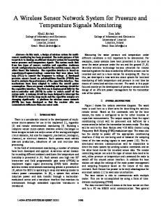
Fig. 5. Seasonal trend in canopy greenness (NDVI) measured using the WSN canopy phenology nodes. Leaf expression begins in May and ends in November. and June. A single node located in the nearest row actually had a significantly higher RSSI than the rest of the network for the duration of the forest green-up. It then demonstrated a sudden decrease in RSSI and afterwards conformed to the communication pattern of the rest of the network. µRSSI ranged between -70 and -75 dBm for the majority of the growing season with a gradual increase as the summer progressed (Fig. 6). A drastic increase in network RSSI from 70 to -63 dBm occurred between October 8 and 11. This sharp transition is not well understood but did correspond to a strong drop in air temperature and high-speed wind gusts. While it is possible that the weather induced an acceleration of leaf removal during the fall leaf senescence, the NDVI data does not reflect this pattern. From then on the network RSSI increased steadily towards a mean of -55 dBm. Given the logarithmic scale of RSSI this represents a nearly 100-fold difference in signal power reception between the spring minimum and the fall maximum RSSI.

ANALYSIS AND OBSERVATIONS

Winter Resilience: Many of the nodes in the network were removed in the fall of 2012 but fifteen nodes were left in place unattended for six months during the harsh winter from November 2012 to April 2013 to test endurance. Batteries were found depleted for three of the nodes but the surviving twelve nodes collected a complete annual data set including the full phenological cycle of the forest. These twelve nodes are the focus of our long-term RSSI analysis. The location of these nodes is shown by grey circles in Fig. 2. They are organized into four rows each 20m further into the forest from the receiver tower. Each row has three columns referred to as left (L), center (C), and right (R) facing the network from the receiver, hereafter referred to by row number (r1-r4) and column location. The raw temperature and PAR data from node r1C in Fig. 4 shows detailed diurnal and seasonal trends for both variables for the full 12 month cycle. As expected, seasonal temperatures lag behind solar radiation levels. Winter temperatures drop below -20°C without any data loss due to node failures. The variability between micro-meteorological observations for different sensor nodes is not discussed here. A.

Temporal Patterns in RSSI

The daily mean network RSSI (µRSSI) was between -64 and -68 dBm prior to the leaf flush in May and showed a general decrease with canopy development throughout May Fig. 6. Time series of the daily mean RSSI for each node and for the average across the sensor network for the spring, summer, and fall of 2013. General seasonality can be seen for the 220-day period. Node r1L showed a drastic unexplained drop at the beginning of June and was excluded from the network mean. Density Distributions: RSSI and micro-meteorological (micromet) sensor data from April 21 to November 30 2013 was further aggregated to hourly and daily means and variances for each of the nine understory nodes. The

Fig. 4. Time series of temperature and photo-synthetically active radiation (PAR) from one node in the sensor network.

305


observations over this 220-day period amounted to 50,000 individual points per sensor, or a total of three million stored entries across the sensor network. As the greenness trend from the tower NDVI nodes shows in Fig. 5. the growing season began in the first week of May and ended in early November. For the analysis, in addition to looking at RSSI trends across the whole season, the RSSI and micromet data were further grouped by forest growth phases, or phenophase, into five periods based on NDVI: spring dormancy, spring green-up, canopy maturity, fall browndown, and fall dormancy. This was done in order to see if the relationships between the biophysical and meteorological variables and network RSSI differed throughout the season. RSSI sample density distributions were created using a Guassian kernel with a bandwidth equal to the twice the sample standard deviation to smooth out minor peaks. Details of this method can be found in the CRAN project density function in the base stats package [26]. Distribution moments are described for both temporal subsets of the mean network RSSI as well as spatial RSSI subsets from individual nodes. Separating the network average RSSI into forest vegetation phenophases reveals a shifting signal density distribution throughout the growing season (Fig. 7). A strongly positive platykurtic distribution is seen for the spring dormancy, greenup, and canopy maturity phenophases with increasing kurtosis and decreasing mean RSSI for these sub-sampled periods. The fall senescence, or brown-down, displays a highly bi-modal RSSI tendency reflecting the sharp transition from low to high RSSI in October. The leafless fall dormancy period also has a bimodality in network RSSI but with a shift towards a higher RSSI than during canopy senescence.

indicates a loss of leaf pigments but not always a dropping of leaves. As such we expect the forest fPAR to correlate better with fall RSSI since it better reflects changes in canopy structure. B.

Spatial Patterns in RSSI

Given our power transmission and reception parameters we expect an ideal RSSI of -61 dBm at 40m and -69.5 dBm at 100m distance between the nodes and base station receiver due solely to free space path loss. Nodes in the first row positioned 40m from the receiver report a significantly lower mean RSSI around -68dBm indicating excess path loss in the environment. However, at 100m distance the nodes in the furthest row from the base station, row 4, report a mean RSSI around -70 dBm revealing almost no excess path loss. One possible explanation for this comes from examining the receiver-node orientation in Fig. 8. The radiation pattern of the tower antenna is directed more towards the back of the network. Alternatively, the apparent two layer vertical structure of the forest may promote horizontal transmission of radio signals while dampening vertical radio propagation. Further work needs to be done in characterizing such an effect as the interaction between forest structural layers and radio propagation could prove important for implementing WSNs over larger distances within forested landscapes.

Fig. 8. WSN node-base layout with slant RF propagation through two layers of dense foliage separated by woody area only. Plot rows R1-R4 separated by 20m. Fig. 9. illustrates the RSSI distribution of the first and fourth row of nodes. The tendency towards a bimodal distribution is more prominent in the more distant nodes than in the nodes closer to the receiver. We might presume that the more distant nodes have more intermittent connections with occasional strong packet delivery resulting in such a distribution. However, as shown in the temporal density histograms, this bimodal distribution was an apparent effect of seasonal transition into the fall monitoring period. With those considerations, it is also relevant to further discuss here the environmental factors in the forest – both biophysical and

Fig. 7. Seasonal variability in the mean network RSSI from April to November 2013. A shift towards lower RSSI values occurs with canopy development. The phenophases selected based on canopy greenness do have representatively distinct radio signal distributions in the spring and summer but the fall brown-down period does not. This is likely due to the fact that a decreasing NDVI in the fall

306


meteorological - capable of inducing seasonal changes in

were daily mean air temperature (T), vapor pressure deficit (VPD) calculated from temperature and relative humidity [Paw method, 1987], wind speed (WND) and down-welling solar radiation (SR) from the meteorological station located on the tower positioned just above the WSN base station. Forest canopy metrics included in the regression analysis were the normalized difference vegetation index (NDVI) and the fraction of absorbed photo-synthetically active radiation (fAPAR). Both of these variables were measured using the optical sensor capabilities of our WSN and are the most commonly used remote sensing phenology indices to indirectly measure canopy leaf area and density [24]. Variables were added to the regression analysis in the following sequence GLM = µRSSI ~ fPAR+NDVI+T+VPD+SR+WND

Figure 9. Seasonal RSSI distributions for three nodes in A) row 1 nearest to the receiver and B) row 4 furthest from the receiver.

Results: Greatest agreement between the relative importance methods was found between the LMG and first approaches. The last and Pratt method resulted in much larger confidence intervals and thus did not help as much in differentiating variable contributions to the model. We still include all four method outputs here in order to assess agreement between them but the LGM is discussed in most detail as it is the most robust regression approach. Across the entire 220-day monitoring period from April through November the regression showed that 68% of the total variability in daily µRSSI can be explained by these six regressors (p