Aug 19, 2003 - Second-harmonic generation in arrays of spherical particles. W. Luis Mochán and Jesús A. Maytorena. Centro de Ciencias Fısicas, Universidad ...
PHYSICAL REVIEW B 68, 085318 共2003兲
Second-harmonic generation in arrays of spherical particles W. Luis Mocha´n and Jesu´s A. Maytorena Centro de Ciencias Fı´sicas, Universidad Nacional Auto´noma de Me´xico, Apartado Postal 48-3, 62251 Cuernavaca, Morelos, Me´xico
Bernardo S. Mendoza Centro de Investigaciones en Optica, Apartado Postal 948-1, 37000 Leo´n, Guanajuato, Me´xico
Vera L. Brudny Departamento de Fı´sica, Facultad de Ciencias Exactas y Naturales, Universidad de Buenos Aires, Buenos Aires, Argentina 共Received 14 November 2002; revised manuscript received 31 March 2003; published 19 August 2003兲 We calculate the optical second harmonic 共SH兲 radiation generated by small spheres made up of a homogeneous centrosymmetric material illuminated by inhomogeneous transverse and/or longitudinal electromagnetic fields. We obtain expressions for the hyperpolarizabilities of the particles in terms of the multipolar bulk susceptibilities and dipolar surface susceptibilities of their constitutive material. We employ the resulting response functions to obtain the nonlinear susceptibilities of a composite medium made up of an array of such particles and to calculate the radiation patterns and the efficiency of SH generation from the bulk and the edge of thin composite films illuminated by finite beams. Each sphere has comparable dipolar and quadrupolar contributions to the nonlinear radiation, and the composite has comparable bulk and edge contributions which interfere among themselves yielding nontrivial radiation and polarization patterns. We present numerical results for Si spheres and we compare our results with recent experiments. DOI: 10.1103/PhysRevB.68.085318
PACS number共s兲: 78.66.⫺w, 73.20.Mf, 42.65.⫺k, 03.50.De
I. INTRODUCTION
Optical second harmonic generation 共SHG兲 in centrosymmetric systems has proved to be a useful spectroscopic probe of surfaces, as the bulk contribution is strongly suppressed due to the symmetry.1 As opposed to other surface techniques, SHG permits the observation of surfaces out of ultrahigh vacuum and in many different ambients. For instance, it may be employed to study buried interfaces. Although most of the theoretical and experimental work has been performed on flat surfaces,2,3 other shapes have also been explored, most notably, spherical particles.4 Recently, SHG was employed to explore a thin composite layer made up of Si spherical nanocrystallites embedded within a SiO2 matrix.5 It was found that the signal came mainly from the nanoparticles, not from the matrix, and that its strength diminished by an order of magnitude when the buried Si/SiO2 interfaces were passivated with hydrogen, thus demonstrating the sensitivity of SHG to the condition of the surface of the particles and its usefulness for studying novel electronic devices. However, experiment showed that the transmitted intensity displayed a peak along the forward direction and with a very narrow angular aperture. This result was unexpected, as previous theory6 indicated that the radiation produced by a single sphere illuminated by a plane wave vanishes identically along the forward direction, as has been corroborated through experiments with suspended colloidal particles.7,8 The theory of Dadap et al.6 mentioned above was developed for spheres illuminated by a plane electromagnetic wave. However, the nonlinear response of the particles actually depends on the nature of the exciting field, as shown by Brudny et al.9 which obtained alternative results for the case of a longitudinal exciting field. In general, the polarizing 0163-1829/2003/68共8兲/085318共14兲/$20.00
field is neither of a pure longitudinal character nor is it a simple plane wave. For example, within a composite, the electric field has longitudinal short range spatial fluctuations10 besides the transverse macroscopic field, and the latter is not necessarily a plane wave. Thus, in the first part of this paper, we generalize the theories above to calculate the quadratic nonlinear response functions of a single small nonmagnetic centrosymmetric sphere illuminated by an arbitrary nonhomogeneous electromagnetic field, constrained only by the absence of external charges within the sphere. Afterward, we employ the resulting hyperpolarizabilities to calculate the macroscopic second order susceptibilities of a composite. Finally, we calculate the SHG from a thin homogeneous slab of this composite illuminated by a focused Gaussian beam, and from an inhomogeneous composite with a density gradient. We find similar bulk and surface contributions to the signal produced by a single sphere. Its dipolar and quadrupolar contributions are also similar, and their relative strength depends on the spatial variation of the polarizing field. As expected, a plane wave produces no coherent SHG exactly along the forward direction, but a finite sized beam produces a nontrivial radiation pattern around the forward direction when it illuminates a homogeneous composite film. The density gradient at the edge of the sample produces a signal that may be larger than that coming from the interior and has different patterns and polarizations, depending on the direction of the incoming electric field with respect to the edge. The paper is organized as follows: In Sec. II we develop the theory for the nonlinear response of a small single sphere. In Sec. III we obtain the macroscopic nonlinear susceptibilities of a homogeneous composite and we employ them to calculate the SHG of a thin film illuminated by a Gaussian beam, and in Sec. IV we take account of the inho-
68 085318-1
©2003 The American Physical Society
´ N, MAYTORENA, MENDOZA, AND BRUDNY MOCHA
PHYSICAL REVIEW B 68, 085318 共2003兲
J (2) , we will also calculate the scalar second Related to Q (2) ˜ of the nonlinear induced charge distribution, moment Q given by ˜ (2) ⫽ ˜␥ q 关 E ex共 0 兲兴 2 . Q
FIG. 1. Nonmagnetic sphere of radius R with dielectric function ⑀ ( ) within a vacuum, being acted upon by an inhomogeneous electric field Eជ ex. The selvedge of width ᐉ is shown as a dark shell.
共3兲
Finally, there is no quadratic magnetization, as no combinaជ ex and ⵜEជ ex can yield an axial vector. As the tion of only E sphere is small, we need not consider further multipolar moments nor higher order spatial derivatives of the field. The purpose of the present section is the calculation of the nonlinear response functions ␥ to lowest order in R, where ␥ ⫽ ␥ e , ␥ m , ␥ q , and ˜␥ q . Assuming that R is small enough, we linearize the field within the sphere as
ជ 0 ⫹rជ •ⵜEជ 0 ⫹O 共 r 2 兲 . Eជ ex共 rជ 兲 ⫽E 12
mogeneity of the density to calculate the radiation from the edge of the film. Within a continuous dipolium model,11 in Sec. V we calculate the response functions and the radiation patterns and intensities corresponding to Si nanospheres, and we compare our results with experiment. Finally, Sec. VI is devoted to a discussion of our results and to conclusions. The details of the derivation presented in Sec. II are included in Appendix A, and the results are compared with those in the literature in Appendix B.
Making an expansion in irreducible tensors,
We first consider a single homogenous, local, isotropic, centrosymmetric, nonmagnetic sphere of radius R centered at the origin, with a linear response characterized by a dielectric function ⑀ ( ). For simplicity we consider that outside the sphere there is only vacuum 共Fig. 1兲. The sphere is acted upon by an inhomogeneous external field Eជ ex(rជ ), oscillating at frequency . We assume that the scale of spatial variation of this polarizing field is much larger than R. Due to quadratic nonlinear optical processes, the sphere may acquire a dipole moment pជ (2) and a quadruJ (2) in response to the external field. The sympole moment Q metry of the sphere implies that, to lowest order in the field gradient, pជ (2) has to be constructed from a combination of ជ ex(0) yielding a vector. The only posibilonly Eជ ex(0) and ⵜE ity is
⫹
冉
ជ ex
⫹ ␥ E 共 0 兲 ⫻ 关共 ⵜ⫻E 共 0 兲兴 .
冉
冊
1 J (2) ⫽ ␥ q E ជ ex共 0 兲 Eជ ex共 0 兲 ⫺ 关 E ex共 0 兲兴 2 J Q 1 . 3
共2兲
共5兲
4 0 iq 1 0 J •rជ , rជ ⫹ Bជ 0 ⫻rជ ⫹ C 3 2 2
共6兲
ជ 0 the external magwhere 0 is the external charge density, B J 0 is a second order symmetric traceless tensor netic field, C and q⫽ /c is the characteristic wave number for the incident field. In the following we will make the reasonable assumption that there is no external charge within the sphere, 0 ⫽0, so that we disregard ␥ . We notice that the first and third term on the right hand side of Eq. 共6兲 are irrotational and may be derived from a scalar potential with angular momenta l⫽1 and 2 respectively, while the second term is solenoidal. Thus, ជ within the sphere is the self-consistent screened linear field E given by ជ 共 rជ 兲 ⫽L 11Eជ 0 ⫹ E
iq 0 1 J 0 •rជ , ជ ⫻rជ ⫹ L 21C B 2 2
共7兲
where L lw are the screening factors for potentials with angular momentum l and frequency w , L lw ⫽
共1兲
J (2) should be written as a traceless, symmetric Similarly, Q ជ ex(0), 9 tensor quadratic in E
冊
1 2 i E 0j ⫹ j E 0i ⫺ ⵜ•Eជ 0 ␦ i j r j , 2 3
and employing Maxwell’s equations,
ជ ex共 0 兲 ⵜ•Eជ ex共 0 兲 ⫹ ␥ e Eជ ex共 0 兲 •ⵜEជ ex共 0 兲 pជ (2) ⫽ ␥ E m ជ ex
we write
1 1 0 ជ ជ0 ជ0 ជ E ex i 共 r 兲 ⫽E i ⫹ 共 ⵜ•E 兲 r i ⫹ 关共 ⵜ⫻E 兲 ⫻r 兴 i 3 2
ជ 0⫹ Eជ ex共 rជ 兲 ⫽E II. NONLINEAR RESPONSE OF A SINGLE SPHERE
共4兲
2l⫹1 , l ⑀ w ⫹l⫹1
共8兲
and we abbreviated ⑀ w ⬅ ⑀ (w ), w⫽1,2. Notice that, as the sphere is nonmagnetic, the solenoidal contribution to the field remains unscreened. Now we chose a particularly simple polarizing field, for ជ0 which Eជ 0 ⫽(0,0,E 0 ) points along the z direction, B 0 0 J ⫽diag(⫺1, ⫽(B ,0,0) points along the x direction, and C ⫺1,2)C 0 /2 produces a potential with cylindrical symmetry
085318-2
PHYSICAL REVIEW B 68, 085318 共2003兲
SECOND-HARMONIC GENERATION IN ARRAYS OF . . .
along the z axis. The hyperpolarizabilities ␥ obtained for these fields may afterwards be employed for the general case. Thus, we write
冉冊 冉 冊 冉 冊 0 ⫺x iq 0 1 0 0 ⫹ B ⫺z ⫹ C ⫺y 2 4 1 y 2z 0
ជ ex
E 共 rជ 兲 ⫽E and
0
共9兲
冉冊 冉 冊 冉 冊
0 ⫺x iq 0 1 0 0 ⫹ B ⫺z ⫹ L 21C ⫺y , 2 4 1 y 2z 共10兲 0
Eជ 共 rជ 兲 ⫽L 11E
0
so we may identify 1 ជ ex共 0 兲 ⫽ 共 0,⫺iqE 0 B 0 ,E 0 C 0 兲 , Eជ ex共 0 兲 •ⵜE 2
共11兲
ជ ex共 0 兲 ⫻ 关 ⵜ⫻Eជ ex共 0 兲兴 ⫽ 共 0,iqE 0 B 0 ,0兲 , E
共12兲
ជ ex共 0 兲兴 2 ⫽ 共 0,iqE 0 B 0 ,E 0 C 0 兲 , ⵜ关E
共13兲
1 ជ ex共 0 兲 ⫺ 关 E ex共 0 兲兴 2 J 1 ⫽diag共 ⫺1,⫺1,2兲共 E 0 兲 2 /3, Eជ ex共 0 兲 E 3 共14兲 and 关 E ex共 0 兲兴 2 ⫽ 共 E 0 兲 2 ,
共15兲
with similar results for the screened field 关Eq. 共10兲兴. ជ b induced by the The macroscopic quadratic polarization P linear field within the bulk of a homogeneous isotropic medium may be written as13
ជ b 共 rជ 兲 ⫽ ␥ ⵜE 2 ⫹ ␦ ⬘ Eជ •ⵜEជ , P
共16兲
ជ b and the FIG. 2. Illustration of the nonlinear bulk polarization P s ជ located immediately outside the sphere. surface polarization P
ជ and the electric Eជ constructed in terms of the displacement D fields at the surface. The advantage of this definition is that it removes the ambiguities as to the position within the selvedge where the fields are to be evaluated. Also, we identify ជ s as the total surface polarization, so that, in contrast to the P ជ b , no further screening of P ជ s is necessary. bulk polarization P This way, we also avoid the ambiguity as to where in the surface should the surface polarization be located; correជ s we place a singular polarization P ជ s ␦ (r sponding to P ⫹ ⫺R ) in vacuum just outside of the sphere 共Fig. 2兲. Assuming that R is much larger than ᐉ, we may safely consider the sphere to be locally flat. Notice that we have already stated that R is smaller than the spatial variation of the field, so in particular, it should be smaller than the optical wavelength . As ᐉ is of the order of the screening depth, typically about an atomic distance, while is commonly two to three orders of magnitude larger, there is a range of sizes R for which the conditions ᐉⰆRⰆ may be obeyed, such as for the 3–10-nm sized particles employed in the experiments of Ref. 5. Thus, we write
冉
where ␥ ( ) and ␦ ⬘ ( ) are the bulk nonlinear response functions. Using Eq. 共10兲 we write
si jk ⫽ s ␦ ir ␦ jr ␦ kr
1 ជ b ⫽ 关 0,⫺iqL 11共 ␦ ⬘ ⫺2 ␥ 兲 E 0 B 0 ,L 11L 21共 ␦ ⬘ ⫹2 ␥ 兲 E 0 C 0 兴 P 2 ⫹O 共 r 兲 .
a
⑀ 21
⫹ 关共 1⫺ ␦ ir 兲共 1⫺ ␦ jr 兲 ␦ kr
⫹ 共 1⫺ ␦ ir 兲 ␦ jr 共 1⫺ ␦ kr 兲兴
共17兲
ជ b , there is a surface quaBesides the bulk polarization P s ជ due to dipolarly allowed processes in a dratic polarizarion P narrow selvedge of width ᐉ where centrosymmetry is locally broken: P si ⫽ si jk F j F k .
共18兲
⫹ ␦ ir 共 1⫺ ␦ jr 兲共 1⫺ ␦ kr 兲 f
共19兲
冊
共 spherical兲
共20兲
in the spherical coordinate basis rˆ , ˆ , ˆ . Here, a⫽a( ), b ⫽b( ) and f ⫽ f ( ) are the dimensionless functions which are commonly employed to parametrize the response of a flat homogeneous surface14,15 that is isotropic within its plane,
ជ , ) is the second order surface susceptiHere si jk ⫽ si jk (R ជ . As in Refs. 9 and 11, we define this bility at position R susceptibility as the response to the continuous field ជ ⬜ 共 Rជ 兲 ⫹Eជ 储 共 Rជ 兲 , Fជ 共 Rជ 兲 ⫽D
b ⑀1
s⫽
共 ⑀ 1 ⫺1 兲 2
64 2 ne
,
共21兲
n is the electronic density, and ⫺e is the electronic charge.
085318-3
´ N, MAYTORENA, MENDOZA, AND BRUDNY MOCHA
PHYSICAL REVIEW B 68, 085318 共2003兲
Integrating Eq. 共17兲 over the bulk and Eq. 共18兲 over the surface of the sphere, and accounting for linear screening at 2 , we can obtain the total second order dipole moment. A similar process permits the calculation of the quadrupole moment. The results of these procedures are 共see Appendix A兲
ជ (2)
p
(2) ⫽ Q zz
2 3 R L 11L 12 ⫽ 15
冉
0 ⫺5iq 关共 ␦ ⬘ ⫺2 ␥ 兲 ⫺2 共 ⑀ 2 f ⫺b 兲 s 兴 E 0 B 0 关 5 共 ␦ ⬘ ⫹2 ␥ 兲 ⫹2 共 2 ⑀ 2 a⫹b⫹3 ⑀ 2 f 兲 兴 L 21E C
32 3 2 R L 11L 22 s 共 ⑀ 2 a⫹3b⫺ ⑀ 2 f 兲共 E 0 兲 2 , 15
s
共23兲
and ˜ s⫽ Q
8 3 2 s R L 11 共 a⫹2 f 兲共 E 0 兲 2 . 3
共24兲
Comparing Eq. 共22兲 with Eq. 共1兲 and employing Eqs. 共11兲 and 共12兲 we finally obtain the dipolar hiperpolarizabilities
␥ e⫽
4 3 R L 11L 12L 21关 5 共 ␦ ⬘ ⫹2 ␥ 兲 ⫹2 s 共 2 ⑀ 2 a⫹b⫹3 ⑀ 2 f 兲兴 15 共25兲
and
␥ m⫽
2 3 R L 11L 12兵 5 关共 ␦ ⬘ ⫹2 ␥ 兲 L 21⫺ 共 ␦ ⬘ ⫺2 ␥ 兲兴 15 ⫹2 s 关共 2 ⑀ 2 a⫹b⫹3 ⑀ 2 f 兲 L 21⫺5 共 b⫺ ⑀ 2 f 兲兴 其 . 共26兲
Similarily, a comparison of Eq. 共23兲 with Eqs. 共2兲 and 共14兲, and of Eq. 共24兲 with Eqs. 共3兲 and 共15兲 yields
␥ q⫽
16 3 2 R L 11L 22 s 共 ⑀ 2 a⫹3b⫺ ⑀ 2 f 兲 5
共27兲
8 3 2 s R L 11 共 a⫹2 f 兲 . 3
共28兲
and ˜␥ q ⫽
A comparison 共see Appendix B兲 of the expressions above with earlier work 共Refs. 9, 6, and 16兲 shows that the present work corrects an oversight in Ref. 9 and extends its results to small spheres made up of isotropic, homogeneous, and centrosymmetric materials with arbitrary bulk and surface response functions ␥ , ␦ ⬘ , a, b, and f and excited by a field with both longitudinal and transverse components. Our results are also a generalization of those of Refs. 6 and 16 to small nonmagnetic spheres immersed in vacuum and excited by a field which is not necessarily a plane wave. In this section we have found expressions for the nonlinear response functions ␥ of a single nanosphere in terms of the intrinsic response of the surface (a, b, f ) and bulk ( ␥ , ␦ ⬘ ) of flat semiinfinite homogeneous and isotropic materials. Thus, we may take advandtage of manifold models and measurements of those intrinsic response functions in order to obtain the nonlinear susceptibility of small particles.
0
0
冊
,
共22兲
III. NONLINEAR RESPONSE OF A COMPOSITE
In Sec. II we obtained the nonlinear response of a single ជ ex. In the present sphere subject to an inhomogeneous field E section we want to look at the response of a composite medium made up of such spheres, such as the nanocrystals that have been studied by Jiang et al.5 In Ref. 5 a thin disordered array of Si spherical nanocrystals within a SiO2 matrix was studied using SHG. The second harmonic radiation was found to be confined to a very narrow (⬇1°) cone and peaked along the forward direction. At first sight, this result is intriguing: The first two contributions to the nonlinear dipole 关Eq. 共1兲兴 of each sphere are null when the sphere is illuminated by a plane wave, while its quadrupole 关Eq. 共2兲兴 would have an axis of cylindrical symmetry lying on the plane wavefront. Therefore, neither the second harmonic 共SH兲 dipole nor the quadrupole moments of the sphere are expected to radiate along the forward direction.6 – 8,16 Thus, it was suggested that the observed radiation originated from density, size and shape fluctuations.5 However, the angular distribution of the radiation is inconsistent with the incoherent signal expected to arise from fluctuations.5,9 Nevertheless, coherent SH radiation may appear when the sample is illuminated with a beam that has a finite waist, as actually employed in Ref. 5, since the in-plane inhomogeneity of the field amplitude might induce further nonlinear sources that might be able to radiate. In Fig. 3 we show schematically the SH dipole moments induced on a composite by a focused fundamental beam. Near the center of the beam, the dipoles point along the nominal propagation direction, and thus they cannot radiate into it. However, as the edge of the illuminated spot is approached, the fundamental amplitude decays, and the corresponding gradient tilts the nonlinear dipoles away from the forward direction. Thus, those dipoles may radiate close to the forward direction. Although the fields produced by dipoles located at opposite sides of the spot might cancel each other exactly along the forward direction, such cancelation is absent at small off-forward scattering angles, yielding a nontrivial intensity distribution. To illustrate this possibility, in this section we calculate the coherent SH radiated by a composite illuminated by a finite beam. We consider thus a system made up of a very narrow disordered array of small spheres distributed with a density n s (rជ ) and illuminated by a finite beam. The place of the external field acting on a given sphere should be taken by the actual external field plus the field produced by other spheres. Thus, we ជ loc. For simplicity, we should replace Eជ ex by the local field E ជ loc with the further ignore the local field effect and identify E M macroscopic field Eជ , which we denote in what follows
085318-4
PHYSICAL REVIEW B 68, 085318 共2003兲
SECOND-HARMONIC GENERATION IN ARRAYS OF . . .
FIG. 4. A Gaussian beam is focused on a spot of radius w 0 on a thin composite film of width l giving rise to a SH scattered radiation. FIG. 3. Schematic representation of the SH dipole moments induced on a composite system illuminated by a focused beam. The SH field radiated at small off-normal directions is indicated, as well as the expected two lobed intensity distribution and the contributions of some dipoles to those lobes.
simply as Eជ as it causes no confusion. The macroscopic nonlinear polarization of the composite medium may be obtained from the nonlinear dipole and quadrupole of each of its component spheres,17 1 1 J (2) ⫺ ⵜn s Q ជ nl ⫽n s pជ (2) ⫺ ⵜ•n s Q ˜ (2) , P 6 6
␥ q ⫺3 ˜␥ q ⵜE 2 , ⫹n b 18
␥q ជ •ⵜEជ E 6
ជ nl ⫽⌫ⵜE 2 ⫹⌬ ⬘ Eជ •ⵜEជ , P
ជ ⫽
共31兲
nb 共 9 ␥ m ⫹ ␥ q ⫺3 ˜␥ q 兲 18
共32兲
⌬ ⬘ ⬅n b 共 ␥ e ⫺ ␥ m ⫺ ␥ q /6兲 ,
共33兲
and
analogous to ␥ and ␦ ⬘ 关Eq. 共16兲兴. Now, we consider a thin sample of width l lying on the z⫽0 plane illuminated by a beam with a finite waist w 0 , as in Ref. 5 共Fig. 4兲. ជ obeys The unscreened SH vector potential A
nl ជ ⫽⫺2i P ជ nl , P t
Aជ T 共 rជ 兲 ⫽⫺2iq
共35兲
冕
ជ ជ
d 3r ⬘
e 2iq 兩 r ⫺r ⬘ 兩 nl ជ 共 rជ ⬘ 兲兴 T . 关P 兩 rជ ⫺rជ ⬘ 兩
共36兲
At large distances r from the illuminated spot we may perជ ជ form the usual approximations 1/兩 rជ ⫺rជ ⬘ 兩 ⬇1/r and e 2iq 兩 r ⫺r ⬘ 兩 ˆ ជ ⬇e 2iqr e ⫺2iqn •r ⬘ with nˆ ⫽(sin cos ,sin sin ,cos ) a unit vector in the direction of rជ , to obtain Aជ T 共 rជ 兲 ⫽⫺2iql
e 2iqr nl T ជK兲 , 共P r
共37兲
where we assumed the film is much narrower than the wavelength, qlⰆ1, and we introduced the two-dimensional Fourier transform
after expanding the curl terms and eliminating the field divergence, where we introduced the response functions ⌫⫽
共34兲
and we solve Eq. 共34兲 to obtain
共30兲
which becomes
4 T ជ , c
where the superscript T denotes the transverse projection of a vector field and ជ is the SH current
共29兲
J is traceless. Within a ˜ as Q where we include the scalar Q homogeneous composite, n s (rជ ) has a constant value n b , and we employ Eqs. 共1兲–共3兲 to write
ជ nl ⫽n b ␥ e Eជ •ⵜEជ ⫹n b ␥ m Eជ ⫻ 共 ⵜ⫻Eជ 兲 ⫺n b P
ជ T ⫽⫺ ⵜ 2 Aជ T ⫹ 共 2q 兲 2 A
ជ Knl ⫽ P
冕
ជ ជ
ជ nl 共 rជ 储 ,z⫽0 兲 e ⫺iK •r 储 , d 2r 储 P
共38兲
ជ ⫽2qnˆ 储 . Actually, much wider films may with wave vector K be considered, as long as phase matching effects are negligible, i.e., ql⌬nⰆ1, with ⌬n⫽n(2 )⫺n( ), and n is the index of refraction of the composite, and as long as beam divergence effects may also be neglected, i.e., lⰆqw 20 . We now realize that the first term in Eq. 共31兲 is purely longitudinal, so it cannot contribute to the radiated field. Thus, substituting into Eq. 共37兲, we obtain the transverse potential
085318-5
Aជ T 共 rជ 兲 ⫽⫺2iql
e 2iqr ជ •ⵜEជ 兲 KT . ⌬ ⬘共 E r
共39兲
´ N, MAYTORENA, MENDOZA, AND BRUDNY MOCHA
PHYSICAL REVIEW B 68, 085318 共2003兲
Using Eq. 共39兲, we have reduced the problem of SH radiation from a thin composite film illuminated by a beam of finite cross section to that of the calculation of the in-plane ជ •ⵜEជ . Fourier transform of the nonlinear driving term E ជ is To proceed, we assume that at z⫽0 the driving field E given by the waist of a Gaussian beam and we assume that its width w 0 is much larger than the wavelength, so that the beam is paraxial around the nominal propagation direction z. Thus, we can ignore the small variations of order K/q in its polarization direction, and we can take a linearly polarized beam of the form
ជ 共 rជ 储 ,0兲 ⫽E 0 e ⫺r 储 /w 0 xˆ , E 2
2
共40兲
where xˆ is the unit vector in the x direction. In this case,
ជ ⫽⫺2 Eជ •ⵜE
E 20 x w 20
e
2 2 ⫺2r 储 /w 0
xˆ
共41兲
is also linearly polarized along xˆ . Since we can consider x to be a transverse direction, normal to the nominal propagation ជ •ⵜEជ ) T ⬇Eជ •ⵜEជ , with the Fourier axis z, we approximate (E transform
ជ •ⵜEជ 兲 KT ⫽ 共E
i 2 2 K w 2 e ⫺K w 0 /8E 20 xˆ . 4 x 0
共42兲
We substitute Eq. 共42兲 into Eq. 共39兲 to obtain the vector potential 2 2 Aជ T 共 rជ 兲 ⫽ q 2 w 20 l cos e ⫺q w 0 /2 2
e 2iqr ⌬ ⬘ E 20 xˆ , r
共43兲
where we wrote the wavevector in terms of the scattering direction and further assumed sin ⬇. ជ r ⫽2iqAជ T is immediatelly obThe radiated electric field E tained from the potential 关Eq. 共43兲兴, and from it we obtain Poynting’s vector Sជ ⫽c 兩 E r 兩 2 nˆ /8 , the SH radiated intensity per unit solid angle into direction nˆ , dI(nˆ )/d⍀⫽r 2 Sជ (rnˆ ) •nˆ and the differential efficiency of SH generation, 1 dI dE ⬅ , d⍀ P 2 d⍀
共44兲
dE 2 2 2 2 ⫽ 共 qw 0 兲 4 2 cos2 e ⫺q w 0 E, d⍀
共45兲
given by
FIG. 5. SH intensity vs angular position of the detector for a disordered array of spheres illuminated by a Gaussian beam of width w 0 and frequency ⫽qc.
The radiated pattern obtained from Eq. 共45兲 is shown in Fig. 5. Notice that there is no radiation along the forward direction, but there is a strong nonlinear signal along two lobes very close to the forward direction, displaced along the incoming polarization direction ⫽0 by an angle ⫾ 2 ⫽⫾1/(qw 0 ). The angular displacement 2 ⫽ 1 /2⫽ 2* / 冑2 where 1 and * 2 are the beam divergence half-angles of the fundamental beam and of the SH field that would have been generated by a homogeneous non-centrosymmetric material, such as the quartz plates usually employed as a reference in SH experiments. We remark that the characteristic angles 1 and * 2 are defined in terms of the angular decay of the fundamental and SH far field amplitudes.18 More directly observable are the corresponding quantities defined in terms of the angular decay of the fundamental and SH intensities, or equivalently, by the second moment of the angular distribution of the intensities, which are 冑2 times smaller. We notice that the efficiency grows as the square of the thickness l of the system, since we assumed it to be very thin. It decreases as the inverse fourth power of the size of the illuminated spot, and for a fixed spot size and out of resonance, it grows as the square of the frequency. On the other hand, if the diffraction angle 1 is kept constant, the efficiency scales as its fourth power and as the sixth power of frequency. The order of magnitude of E may be estimated from Eqs. 共20兲, 共21兲, 共25兲, 共26兲, 共27兲, 共28兲, 共33兲, and 共47兲. Far from resonance, the hypolarizabilities ␥ are of order R 3 s 关Eqs. 共25兲, 共26兲, 共27兲, and 共28兲兴, and s is of order 10⫺3 /ne. The electronic density n of a solid is typically of order 10/a B3 where a B is Bohr radius. Thus, from Eq. 共33兲, ⌬ ⬘ ⬃10⫺2 f b a B3 /e, where f b ⫽4 n b R 3 /3 is the filling fraction of the spheres. Substituting in Eq. 共47兲 and writing the result in terms of 1 ⫽2/qw 0 , we finally obtain
where P is the incoming power, P⫽
c 8
冕
d 2 r 储 兩 E 共 rជ 储 ,0兲 兩 2 ⫽
cw 20 16
E⫽10⫺2 共 qa B 兲 4 共 ql 兲 2 f 2b 41 兩 E 0兩 2,
共46兲
and E is the integrated efficiency over the whole solid angle: E⬅
1 P2
冕
dI 64 2 共 ql 兲 2 d⍀ 兩 ⌬ ⬘兩 2. ⫽ d⍀ c w 40
共47兲
1
1 e /a B c/a B 2
⬇10⫺4 共 qa B 兲 4 共 ql 兲 2 f 2b 41 W⫺1 ,
共48兲
where is a pure number which we expect to be of order unity, though it may vary by a couple of orders of magnitude due to the high powers of dimensionless numbers which appear implicitly in Eq. 共47兲. The reasonable choice qa B
085318-6
PHYSICAL REVIEW B 68, 085318 共2003兲
SECOND-HARMONIC GENERATION IN ARRAYS OF . . .
⬇10⫺2 , ql⬇1, f b ⬇10⫺1 , and 1 ⬇1°⬇2⫻10⫺2 yields an efficiency E⬇10⫺24 W⫺1 . For thicker composites, for which ql is larger than order 1, phase matching effects might have to be accounted for. Qualitatively, this may be accomplished simply by replacing l 2 in the previous equations by the phase mismatch factor, i.e., l 2 → 兩 sin共 ql⌬n 兲 / 共 q⌬n 兲 兩 2 .
共49兲
Additional changes would be necessary for very thick samples with l⬇qw 20 or larger, for which the divergence of the fundamental and SH beams within the sample have to be accounted for. In the experiments of Jiang et al. described earlier5 l⬇10/q was not so large as to produce phase mismatch effects and the other parameters were close to those mentioned above. On the other hand, about 100–300 SHG 3.1-eV photons were detected per second from a sample illuminated by 2.5⫻105 100–200 fs, 1- J pulses each second,19 yielding the measured efficiency E⬇10⫺23 W⫺1 , in good agreement with the estimation above. The ubiquitous randomness within composites yields necessarily some incoherent radiation. Thus, it is instructive to estimate the efficiency of the incoherent SHG Einc and to compare it with its coherent counterpart E 关Eq. 共48兲兴. As the dipolar and quadrupolar radiation produced by a single sphere are similar, we estimate the intensity of the SH signal produced by an individual sphere through Larmor’s formula 4 (2) 2 ) /3⬃10cq 6 ( s ) 2 R 6 E 40 /3, where we used P (2) 1 ⬃c(2q) (p Eq. 共1兲 and we estimated ␥ ⬃ s R 3 and E 0 ⵜE 0 ⬃qE 20 . Multiplying by the number of illuminated spheres ⬃n s lw 20 and dividing by the square of the incident power Eq. 共46兲, we obtain the incoherent efficiency Einc⬃ f b 共 qa B 兲 4
q 2 lR 3 w 20
1 1 , 2 c/a B e /a B
served SH intensity as the beam crossed the edge of the composite was about an order of magnitude larger than the signal from well within the composite, instead of interpolating smoothly between the signal from the interior and the practically inexistent signal from the exterior, as could have been naively expected. Furthermore, the signal displayed strong oscillations close to the edge. Thus, in this section we concentrate our attention on the calculation of the SH radiation from the lateral edge of a thin composite made of small spheres, such as that considered in the previous section 共see Fig. 6兲. Accounting for the variation of the density n s ⬅n b (x,y) across the illuminated spot, from Eq. 共29兲 we obtain
ជ nl ⫽⌬ ⬘ Eជ •ⵜEជ ⫹⌫ⵜ 共 E 2 兲 ⫺n b P 共50兲
where we employed the estimate for s given above, so that Einc 共 qR 兲 3 共 qw 0 兲 2 ⬃101 . E 共 ql 兲 f B
FIG. 6. A Gaussian beam is focused on the edge of a thin composite, as that in Fig. 4, producing SH radiation 共light arrows兲. The gradient of the density of spheres ⵜn s close to the edge is indicated 共heavy arrow兲.
共51兲
Substituting the parameters corresponding to the experiment of Jiang et al. 共Ref. 5兲 mentioned above, we obtain that the coherent and incoherent contributions have comparable SH efficiency. However, the incoherent radiation is distributed over a wide solid angle, according to a superposition of dipolar and quadrupolar radiation patterns,9 while the coherent radiation has a very narrow distribution close to the forward direction 共Fig. 5兲 and, thus, it has a much larger intensity. On the other hand, the dependence of the incoherent signal on f b and R differs20 from that of the coherent signal, and for diluted samples such as suspensions, the incoherent radiation may dominate.7,8,20 IV. NONLINEAR RESPONSE AT THE EDGE OF THE COMPOSITE
Another intriguing observation was reported in Ref. 5 regarding the intensity of the SH signal as the fundamental beam was scanned laterally through the sample. The ob-
␥m 2 ␥q ជ Eជ •ⵜ , E ⵜ ⫺n b E 2 6 共52兲
instead of Eq. 共31兲, where is a function which varies from 0 outside the composite to its bulk value 1 within. Without loss of generality we take the edge along the y axis, so that ⫽ (x), and we write ⵜn s ⫽n b (d /dx)xˆ ⬅n b ⬘ (x)xˆ . Then, Eq. 共52兲 reduces to
ជ nl ⫽⌬ ⬘ Eជ •ⵜEជ ⫹⌫ⵜ 共 E 2 兲 ⫹⌼ ⬘ 共 x 兲 xˆ E 2 , P
共53兲
ជ points in where ⌼ depends on whether the external field E the direction parallel ( ⫽ 储 ) or perpendicular ( ⫽⬜) to the gradient of n s , ⌼ 储 ⫽⫺n b
冉
冊
␥m ␥q ⫹ , 2 6
⌼⬜ ⫽⫺n b
␥m . 2
共54兲
The far field is now given by Aជ T 共 rជ 兲 ⫽⫺2iql
e 2iqr ជ •ⵜEជ ⫹⌼ ⬘ xˆ E 2 兲 KT 共 ⌬ ⬘ E r
共55兲
instead of Eq. 共39兲. To proceed, we chose a smooth density profile and we assume that its spatial scale of variation is larger than w 0 , so we approximate it by a linear profile
085318-7
共 x 兲 ⫽ 0 ⫹x/L,
共56兲
´ N, MAYTORENA, MENDOZA, AND BRUDNY MOCHA
PHYSICAL REVIEW B 68, 085318 共2003兲
with 0 representing the relative density at the center of the beam, which we take without loss of generality at x⫽0, and L is a distance of the order of the width of the edge. Substituting Eq. 共56兲 into Eq. 共55兲, performing the Fourier transform under the assumption of a small illuminated spot (w 0 ⬍L), and calculating the resulting radiation pattern, we finally obtain 2
2
冏
w0 dE储 8 e ⫺4 / 1 2 ⫽ Eb cos ⫹i 2 d⍀ 1 0L 1
冉
1 2 ⌼储 ⫻ ⫺2 2 cos2 ⫺ 2 1 ⌬⬘
共57兲
,
冋 冉 冊 冉 冏 冏 冊册 冏 冋冏 冏 冏冉 冊册 冋 冉 冊 冉 冏 冏 冊册 2
2
dE⬜ 8 e ⫺4 / 1 ⫽ E d⍀ b 21 ⌼⬜ ⌬⬘
2
3 ⌼储 ⌼储 ⫺Re ⫹2 8 ⌬⬘ ⌬⬘
共58兲
,
w0 2 2 sin ⫺i sin 2 1 0 L 21
2
,
1 ⌼⬜ ⫹2 8 ⌬⬘
2
w0 0L
共59兲
2
,
共60兲
dE储 储 dE储 ⫽ , d⍀ d⍀
共61兲
E储 储 ⫽E储 ,
共62兲
dE⬜ 储 ⫽0, d⍀
共63兲
E⬜ 储 ⫽0,
共64兲
冏 冏冉 冊 冉 冊冏 冏 2
2
dE储⬜ 8 e ⫺4 / 1 ⌼⬜ ⫽ Eb d⍀ 21 ⌬⬘ w0 E储⬜ ⫽2Eb 0L 2
冋 冉 冊册
E⬜⬜ ⫽Eb 1⫹
where Eb is the total efficiency of a homogeneous film 关Eq. 共47兲兴 but evaluated at the nominal density n b 0 at the center of the illuminating beam, i.e., Eb ⫽ 20 E. Here, dE /d⍀ and E denote the differential and total SHG efficiencies for the case in which the incoming polarization points along the direction ⫽ 储 ,⬜. More detailed information may be obtained by analyzing the outgoing beam with a linear polarizer. In this case we obtain
2
FIG. 7. Absolute value of the nonlinear response functions 兩 ␥ 兩 , where ␥ ⫽ ␥ e , ␥ m , ␥ q , and ˜␥ q for a single Si nanosphere. The labels E 1 and E 2 denote the critical points of Si, E 1 /2 and E 2 /2 denote their subharmonics, and D/2 and Q/2 denote the subharmonics of the dipolar and quadrupolar resonances, for which Re ⑀ 2 ⫽⫺2 and ⫺3/2.
2
w0 0L
E⬜ ⫽Eb 1⫹
2
2
w0 0L
E储 ⫽Eb 1⫹
⫹
冊冏
2
冏
2
2
⌼⬜ ⌬⬘
w0 0L
1 w0 8 0L
2
,
共68兲
where dE /d⍀ and E denote the differential and total efficiencies, with and denoting the outgoing and the incoming polarizations respectively. V. RESULTS FOR SI NANOCRYSTALLITES
As Ref. 5 presents experimental results for Si nanospheres, in this section we apply to them some of our previous results. For simplicity, we calculate the surface and bulk nonlinear response functions of Si from its linear dielectric function21 using the continuous dipolium model.11 In Fig. 7 we show the nonlinear response of a single Si nanosphere, obtained from Eqs. 共B4兲–共B8兲. Some structures visible in this figure are inherited from the linear bulk responses ⑀ 1 and ⑀ 2 and thus appear at the fundamental or at the subharmonic frequencies of the critical points of the Si joint density of states. Further structures are due to the nonlinear surface response a.9,11 The resonances of
2
共65兲
,
2
共66兲
,
冏
2
w0 2 dE⬜⬜ 8 e ⫺4 / 1 2 sin ⫺i sin 2 , ⫽ Eb d⍀ 1 0 L 21 21
共67兲
FIG. 8. Squared absolute value 兩 ⌬ ⬘ 兩 2 of the bulk nonlinear response of a homogeneous composite made up of spherical Si inclusions.
085318-8
PHYSICAL REVIEW B 68, 085318 共2003兲
SECOND-HARMONIC GENERATION IN ARRAYS OF . . .
FIG. 9. Absolute value ⌼ /⌬ ⬘ of the quotient between the edge and the bulk response functions at the edge of a composite made of Si nanospheres for two directions of the incoming polarization, parallel ( ⫽ 储 ) and perpendicular( ⫽⬜) to the density gradient ⵜn s .
the screening factors L l2 are too damped due to the finite imaginary part of ⑀ 2 and the resonances of L l1 are outside of the spectral region shown in Fig. 7. In Fig. 8 we show the bulk response ⌬ ⬘ calculated for a homogeneous composite made of n b Si nanospheres per unit volume, calculated by substituting the nonlinear response of each Si particle, shown in Fig. 7, into Eq. 共33兲. We notice that only its squared magnitude 兩 ⌬ ⬘ 兩 2 enters the differential and total SHG efficiencies 关Eqs. 共45兲 and 共47兲兴, and that the composite response ⌫ does not contribute. Fig. 8 shows that the efficiency increases almost monotonically up to about 5.5 eV, but has many features corresponding roughly to those displayed in Fig. 7. However, ␥ are complex quantities and they interfere among themselves, leading to a richer structure in Fig. 8. As shown by Eqs. 共57兲–共68兲, the differential and total SH efficiencies at the edge of a thin composite layer depend on the nominal efficiency of a homogeneous composite Eb and on the quotients ⌼ 储 /⌬ ⬘ and ⌼⬜ /⌬ ⬘ , which together with the relative widths w 0 and L of the beam and the edge control the relative contribution from the field and the density gradients. Figure 9 illustrates the frequency dependence of these relative contributions.
In Fig. 10 we show the SH radiation patterns from the edge of the composite film. The incoming energy ប ⫽1.55 eV and polarization 储 are the same as in the experiment of Jiang et al.5 We assumed the nominal beam focused at the middle of the edge, with a nominal density n s ⫽0.5n b . We notice that for a wide edge, or equivalently, for a thin beam, the differential efficiency is the same as the two lobbed radiation pattern of Fig. 5 for a homogeneous film 共left panel兲. However, for a wider beam or a thinner edge a new contribution coming from the gradient ⵜn s of the density appears, filling the minimum between the two lobes 共middle panel兲. Furthermore, the interference between the bulk-like and edge signals produces an asymmetry between both lobes; the lobe that leans towards ⵜn s is smaller. As could be expected from Fig. 9, the degree of asymmetry depends on the frequency. Already for w 0 /L⬇0.1 the gradient contribution dominates and the two-lobed structure is almost lost 共right panel兲, although a slight asymmetry is still visible. In this case the peak is about twice as high as those for the homogeneous film. In Fig. 11 we show the corresponding results but for polarization perpendicular to ⵜn s , i.e., along the edge. As ⌼⬜ ⬍⌼ 储 at ប ⫽1.55 eV, higher values of w 0 /L are required before the gradient contribution becomes visible. In this case, the two lobes are rotated with respect to those of Fig. 10 and retain their symmetry. The gradient and the bulklike contributions are polarized along and normal to ⵜn s respectively. Thus the relatively small gradient contribution in Fig. 11 may be isolated by analyzing the outgoing beam with a linear polarizer. The polarized radiation pattern dE储⬜ /d⍀ is a simple Gaussian 关Eq. 共65兲兴 for all values of w 0 /L. VI. DISCUSSION AND CONCLUSIONS
In this paper we first obtained the quadratic optical response of a single centrosymmetric nonmagnetic isotropic sphere illuminated by an inhomogeneous electromagnetic field. As we did not make assumptions about the nature of the polarizing field, our results may be employed for both transverse and longitudinal exciting fields. Thus they consti-
FIG. 10. SH radiation patterns dE储 /d⍀ from the edge of a composite thin film made up of Si nanospheres for various values of the beam width w 0 and the edge size L, w 0 /L⫽0.01, 0.05, and 0.1. The energy of the incoming photons is ប ⫽1.55 eV and we chose the nominal density at half the bulk value n s ⫽0.5n b . For reference, small vertical bars corresponding to the same fixed height 0.5Eb are shown in each panel. The arrow indicates the direction of the density gradient. 085318-9
´ N, MAYTORENA, MENDOZA, AND BRUDNY MOCHA
PHYSICAL REVIEW B 68, 085318 共2003兲
FIG. 11. SH radiation patterns dE⬜ /d⍀ as in Fig. 10 but for a polarization perpendicular to the density gradient ⵜn s . The vertical bar references have the same size as in Fig. 10.
tute a generalization of previous works.9,6,16 The hyperpolarizabilities ␥ e , ␥ m , ␥ q , and ˜␥ q were calculated to lowest order (R 3 ) in the size of the particles and were written in terms of their bulk and surface second order susceptibilities under the assumption that the curvature was small enough that the surface could be considered locally flat. As has been discussed previously,6 each individual sphere is unable to radiate in the forward direction when illuminated by a plane wave. However, the experimental observation of a very narrow SH peak in the forward direction from composite films made up of spherical Si nanocrystals embedded in SiO2 was recently reported.5 To understand its origin, we applied our results to the calculation of the response of composites illuminated by a focused Gaussian linearly polarized beam. We obtained that neither in this case can there be radiation exactly in the forward direction. However, the radiation pattern shows two narrow lobes displaced along the polarization direction by a small angle of the order of the diffraction-induced angular divergence of the linear far field. The forward peak reported experimentally for an array of Si nanospheres5 may have been confused with one of these lobes.19 We discussed the dependence of the SH differential and total efficiencies on parameters such as the width of the film, the density of inclusions, and the waist of the beam. The experiment also showed that the signal may be enhanced at the lateral edge of finite films. Thus, we calculated the SH radiation produced at a non-homogeneous film. We found bulklike contributions and contributions due to the gradient of the inclusion density. The radiation patterns, the dependence on the input polarization, the output polarization directions, and the spectral features of both contributions differ in general, and they arise from different combinations of the individual sphere’s response functions. These contribu-
ជ s⫽ s P
冉
共 acos2 ⫹ f sin2 兲
⫺2b sin cos
⫹iq
s
冉
0
冊
f sin sin ⫺b cos sin ⫺b cos cos 2
1 2 L 11 共 E 0 兲2⫹ s 2
冊
冉
tions may interfere among themselves, yielding nontrivial patterns which may be modified by changing the frequency, the waist of the illuminating beam, or the sharpeness of the edge. By analyzing the polarization of the outgoing beams gradient and bulk-like contributions may be separated, facilitating the analysis of the response functions. Calculations for a Si nanosphere composite within a simple dipolium model11 agree qualitatively with the experimental observations.5 The solid-angle resolved SH patterns radiated by the bulk and edge we have calculated have not been explored experimentally yet. The bulk radiation of the composite depends on a single parameter ⌬ ⬘ , which in turn depends, through the hyperpolarizabilities ␥ , on the bulk and surface response functions ␦ ⬘ , ␥ , a, b, and f, of an individual sphere. As the radiation from the edge involves different combinations ⌼ of the above response functions, proper measurements might provide additional information to partially disentangle the separate contributions. We hope that this work will stimulate further experiments and theory. ACKNOWLEDGMENTS
We are grateful to Michael Downer for showing us his results previous to publication and to him and to Tony Heinz for useful discussions. We acknowledge the support from DGAPA-UNAM under Grant Nos. IN110999 and IN117402 共W.L.M. and J.M.兲, from Conacyt under Grant No. 36033-E 共B.M.兲, and from Fundacio´n Antorchas 共VLB兲. V.L.B. is also with CONICET, Argentina. APPENDIX A: SECOND ORDER DIPOLE AND QUADRUPOLE MOMENTS OF A SPHERE
To obtain the surface polarization, we substitute Eqs. 共10兲, 共19兲, 共20兲, and 共21兲 into Eq. 共18兲, leading to
关 a cos 共 3 cos2 ⫺1 兲 ⫹3 f cos sin2 兴
L 11RE 0 B 0 ⫹O 共 R 2 兲
b sin 共 1⫺6 cos2 兲 0 共 spherical兲 .
085318-10
冊
L 11L 21RE 0 C 0
共A1兲
PHYSICAL REVIEW B 68, 085318 共2003兲
SECOND-HARMONIC GENERATION IN ARRAYS OF . . .
Now we calculate the dipole and quadrupole moments proជ b and surface P ជ s polarizations. Integratduced by the bulk P ing Eq. 共17兲 within the volume of the sphere we obtain the bulk contribution to the nonlinear dipole moment, given to lowest order in R by pជ b ⫽
2 3 R L 11关 0,⫺iq 共 ␦ ⬘ ⫺2 ␥ 兲 E 0 B 0 ,L 21共 ␦ ⬘ ⫹2 ␥ 兲 E 0 C 0 兴 . 3 共A2兲
ជ s of order O(R 0 ) We notice that there is a contribution to P so that even a constant external field induces a nonlinear polarization at the surface of the sphere due to the local loss of centrosymmetry. However, once we convert Eq. 共A1兲 to Cartesian coordinates and integrate over the surface, it yields a null contribution to the total nonlinear dipole of the sphere, as the sphere is globally centrosymmetric. On the other hand, converting to Cartesian coordinates and integrating the second and third terms on the right hand side of Eq. 共A1兲 yields a finite surface contribution to the nonlinear dipole pជ s ⫽pជ s储 ⫹pជ ⬜s , where pជ s储 ⫽
共A3兲
冉
0 4 3 s 0 0 R L 11 ⫺5iqbE B 15 bL 21E 0 C 0
where V denotes the volume of the sphere, and ⍀ is the solid angle. To lowest order, the bulk polarization is constant, J b to quadrupole 共A7兲 of orleading to a bulk contribution Q 4 der O(R ), which moreover vanishes from symmetry. The lowest order surface polarization is independent of R and yields a quadrupole of order R 3 . From Eq. 共A1兲, we notice that this term is independent of B 0 and C 0 and is produced only by the constant part of the external field Eជ 0 . Thus, in the J s we may assume cylindrical symmetry calculation of Q J s ⫽diag(⫺1,⫺1,2)Q s /2. Subaround the z axis and write Q zz stituting Eq. 共A1兲 into Eq. 共A8兲 and performing the integral, we obtain s s s ⫽Q zz Q zz 储 ⫹Q zz⬜ ,
where
冊
冉
0 5iq f E 0 B 0 共 2a⫹3 f 兲 L 21E C 0
0
冊
共A5兲
冕
d 3 r 共 rជ 兲共 3rជ rជ ⫺r 2 J 1 兲.
共A6兲
We write the density in terms of the polarization ជ , and we include in P ជ the quadratic bulk contribu⫽⫺ⵜ• P b ជ tion P 关Eq. 共17兲兴 and the singular surface polarization ជ s ␦ (r⫺R ⫹ ) 共Eq. 共A1兲兲. Integrating Eq. 共A6兲 by parts we P obtain a bulk contribution J b⫽ Q
冕
V
ជ b rជ ⫹rជ P ជ b 兲 ⫺2 P ជ b •rជ J d 3r 关 3共 P 1 兴,
共A7兲
and a surface contribution J s ⫽R 3 Q
冕
ជ s rˆ ⫹rˆ P ជ s 兲 ⫺2 P ជ s •rˆ J d 2⍀ 关 3共 P 1 兴,
32 3 2 s R L 11 共 a⫺ f 兲共 E 0 兲 2 15
共A11兲
ជ ⬜s . originates from P Finally, we calculate the second moment of the quadratic induced charge ˜⫽ Q
冕
共A8兲
d 3 r 共 rជ 兲 r 2 .
共A12兲
As we did above, we write in terms of the polarization and integrate by parts to obtain a bulk contribution, ˜ b ⫽2 Q
ជ ⬜s perpendicular to the surface. Both from the polarization P contributions are proportional to the volume of the sphere and we neglect terms of higher order in R. We now proceed to the calculation of the quadrupole moment: J⫽ Q
共A10兲
ជ s储 and originates from P
ជ s储 parallel to the surface, originates from the polarization P and 4 3 s R L 11 pជ ⬜s ⫽ 15
32 3 2 s R L 11 b 共 E 0 兲 2 5
s Q zz 储⫽
s Q zz⬜ ⫽
共A4兲
共A9兲
冕
ជ b •rជ , d 3r P
共A13兲
and a surface contribution, ˜ s ⫽2R 3 Q
冕
ជ s •rˆ , d 2⍀ P
共A14兲
in analogy to Eqs. 共A7兲 and 共A8兲. As above, to order O(R 3 ) there is no bulk contribution. The surface contribution, ˜ s⫽ Q
8 3 2 s R L 11 共 a⫹2 f 兲共 E 0 兲 2 , 3
共A15兲
may be obtained by substituting the first term on the right hand side of Eq. 共A1兲 in Eq. 共A14兲. The only finite contribution to Eq. 共A15兲 originates from the perpendicular surface ជ ⬜s . polarization P To get the total multipole moments of the sphere we cannot simply add the bulk and surface contributions 共A2兲, 共A4兲, 共A5兲, or 共A10兲, 共A11兲, as we have yet to account for the ជ b and P ជ s within screening at 2 of the fields produced by P the bulk of the sphere. To this end we briefly follow Ref. 9. Since there is no magnetic moment induced and we assumed the sphere to be very small, in its immediate neighborhood
085318-11
´ N, MAYTORENA, MENDOZA, AND BRUDNY MOCHA
PHYSICAL REVIEW B 68, 085318 共2003兲
˜ (2) , in the following we will neglect it. Actually, it ment Q turns out that b is a constant so it has no contribution to the terms with l⫽0, for which Eq. 共A16兲 becomes Laplace’s equation, with solution
再
F lm r l 4 ⫻ lm 共 r 兲 ⫽ 2l⫹1 q lm /r l⫹1
共 inside兲 共 outside兲 ,
共A19兲
where we identify q lm with the spherical components of the multipolar moments.22 The coefficients q lm and F lm are determined by boundary conditions 共A17兲 and 共A18兲, which become q lm R l⫹1
P⬜s
FIG. 12. Illustration of the surface polarization , and the surface charge density b and s储 produced by the bulk polarization ជ b and the surface polarization P ជ s储 , respectively. The figure correP sponds qualitatively to Fig. 2. Due to screening, additional charges are induced at the boundary of the sphere with dielectric response ⑀ 2 , but they are not shown. There is no additional screening surface polarization.
⫺F lm R l ⫽ 共 2l⫹1 兲共 P⬜s 兲 lm ,
共A20兲
and 共 l⫹1 兲
q lm R l⫹2
b ⫹l ⑀ 2 F lm R l⫺1 ⫽ 共 2l⫹1 兲共 lm ⫹ s储 lm 兲 ,
共A21兲
and yield we can neglect retardation and describe the selfconsistent field in terms of a quasistatic scalar potential . The equation obeyed by is ⵜ 2 ⫽
再
⫺4 / ⑀ 2
共 inside兲
0
共 outside兲 ,
b
共A16兲
where the unscreened bulk charge density at 2 , b ជ b , is divided by ⑀ 2 to yield the screened charge ⫽⫺ⵜ• P density. The boundary conditions obeyed by are
共 R ⫹ 兲 ⫺ 共 R ⫺ 兲 ⫽4 P⬜s
共A17兲
and
共 R ⫹ 兲 ⫺ ⑀ 2 共 R ⫺ 兲 ⫽⫺4 . R R
b ⫹ s储 lm 兲 R l⫹2 ⫹l ⑀ 2 共 P⬜s 兲 lm R l⫹1 兴 q lm ⫽L l2 关共 lm b s ⫽q lm ⫹q s储 lm ⫹q⬜lm ,
with L l2 the screening factor 共8兲 at the second harmonic for the angular momentum l. Here we have identified a bulk b ⬀ b ⬀ P b , a surface contribution originated contribution q lm in the tangential surface polarization q s储 lm ⬀ s储 ⬀ P s储 , and a surface contribution originated in the perpendicular polarizas ⬀ P⬜s . tion q⬜lm Setting ⑀ 2 →1, L l2 →1 in Eq. 共A22兲 we obtain the unscreened multipolar moments, which are then simply compared to their screened counterparts, yielding
共A18兲
Equation 共A17兲 expresses the discontinuity of the potential due to a singular surface polarization, while Eq. 共A18兲 expresses the discontinuity of the normal component of the field due to the surface charge ⫽ b ⫹ s储 which has a bulk ជ b •rˆ and a surface originated originated contribution b ⫽ P s s ជ contribution 储 ⫽⫺ⵜ储 • P 储 produced by the parallel compoជ s 共see Fig. 12兲. nent of the surface polarization P s ជ As discussed above, P denotes the self-consistent surface polarization and therefore, there is no additional screening ជ s may induce a field within the contribution to it. However, P sphere, and this field may lead to an additional induced bulk polarization and to bulk and surface screening charges. These are accounted for by the factors ⑀ 2 in Eqs. 共A16兲 and 共A18兲. Now we expand all quantities in Eqs. 共A16兲–共A18兲 in terms of spherical harmonics Y lm ( , ) as ⫽ 兺 lm Y lm , b b ⫽ 兺 lm Y lm , P⬜s ⫽ 兺 ( P⬜s ) lm Y lm , etc. Since b contributes terms of at least order O(R 4 ) to the dipolar moment pជ (2) and O(R 5 ) to the quadrupolar moment Q (2) and the second mo-
共A22兲
b b q lm 共 screened兲 ⫽L l2 q lm 共 unscreened兲 ,
共A23兲
q s储 lm 共 screened兲 ⫽L l2 q s储 lm 共 unscreened兲 ,
共A24兲
s s q⬜lm 共 screened兲 ⫽L l2 ⑀ 2 q⬜lm 共 unscreened兲 .
共A25兲
and
Thus, the total dipole (l⫽1) and quadrupole (l⫽2) moments may be obtained from the unscreened moments obtained previously 关Eqs. 共A2兲, 共A4兲, 共A5兲, 共A10兲, and 共A11兲兴 by multiplying by the screening factor L l2 at 2 . Those multipoles that originate in the perpendicular surface polarization P⬜s 关Eqs. 共A5兲 and 共A11兲兴 are to be further multiplied by ⑀ 2 . After screening and adding the bulk 关Eq. 共A2兲兴 and surface 关Eqs. 共A4兲 and 共A5兲兴 contributions, we obtain the total nonlinear dipole pជ (2) induced in the sphere, given by Eq. 共22兲. Similarly, we screen and add the contributions to the induced quadrupole 关Eqs. 共A10兲 and 共A11兲兴 to obtain the ˜ s is total quadrupole moment 共23兲. Finally, we notice that Q determined only by the l⫽0 contribution to the normal polarization ( P⬜s ) 00 , and that the field produced by this polar-
085318-12
PHYSICAL REVIEW B 68, 085318 共2003兲
SECOND-HARMONIC GENERATION IN ARRAYS OF . . .
ization does not penetrate the system and is therefore not ˜ (2) coincides with Q ˜ s 关Eq. 共A15兲兴, and is screened. Thus, Q given in Eq. 共24兲 for the benefit of the reader.
We complete the expressions above by stating in our notation the values of a, b, and f corresponding to the model of Ref. 11, a 共 兲 ⫽2 共关 ⑀ 2 ⫺ ⑀ 1 兴关 2 ⑀ 1 ⫺ ⑀ 2 ⫺ ⑀ 1 ⑀ 2 兴
APPENDIX B: COMPARISON WITH EARLIER WORK
In Ref. 11 a simple model for the nonlinear response of a centrosymmetric dielectric was developed, which lead to explicit analytic expressions for the nonlinear bulk and surface response functions in terms of the linear response. The model consists of a continuous distribution of polarizable entities, each of which responds nonlinearly to the gradient of the field as a forced harmonic oscillator. Although very crude, that model is a convenient first step for the analysis of real systems, as it permits the actual calculation of spectra from the knowledge of only ⑀ ( ), which can be obtained experimentally or through microscopic calculations. In the present section we employ that model to obtain definite expressions for the response of small spheres. From Eqs. 共12兲, 共13兲 and 共14兲 of Ref. 11 we obtain the bulk polarization
ជ b⫽ P
n n ␣ ␣ 共 ⵜE 2 ⫺4Eជ •ⵜEជ 兲 ⫹ ␣ 21 Eជ •ⵜEជ , 2e 1 2 2e
共B1兲
where n is the number density of polarizable ‘‘molecules’’ within the bulk and ␣ w ⫽ ␣ (w ) is the linear polarizability of each one, related to the dielectric function through ⑀ w ⫽1⫹4 n ␣ w . Comparing Eq. 共B1兲 with Eq. 共16兲 we identify n ␣ ␣ 2e 1 2
共B2兲
n ␣ 共 ␣ ⫺4 ␣ 2 兲 . 2e 1 1
共B3兲
␥⫽ and
␦ ⬘⫽
⫹ 关 ⑀ 1 兴 2 关 1⫺ ⑀ 2 兴 log关 ⑀ 1 / ⑀ 2 兴 兲 / 关 ⑀ 2 ⫺ ⑀ 1 兴 2 ,
⑀ 1 ⫺1 3 关 5 共 ⑀ 1 ⫺2 ⑀ 2 ⫹1 兲 8 ne 共 ⑀ 1 ⫹2 兲共 2 ⑀ 1 ⫹3 兲共 ⑀ 2 ⫹2 兲 ⫹ 共 ⑀ 1 ⫺1 兲共 2 ⑀ 2 a⫹b⫹3 ⑀ 2 f 兲兴 R 3 ,
␥ m⫽
f ⫽0.
共B10兲
Our ␥ e and ␥ q 关Eqs. 共B4兲 and 共B6兲兴 are similar to those obtained for pure longitudinal fields, given by Eqs. 共40兲 and 共41兲 of Ref. 9. However, in Ref. 9 no account was taken of the polarization linearly induced within the interior of the sphere by the field originated at the surface nonlinear polarization. Thus, a factor of L 12 is missing from the surface term of Eq. 共40兲 and a factor L 22 is missing from the surface term of Eq. 共41兲 in Ref. 9. Furthermore, an additional factor of ⑀ 2 multiplying the surface response functions a and f is also missing from Ref. 9. Therefore, Sec. II corrects an oversight in Ref. 9 and extends its results to small spheres made up of isotropic, homogeneous, and centrosymmetric materials with arbitrary bulk and surface response functions ␥ , ␦ ⬘ , a, b, and f and excited by a field with both longitudinal and transverse components. Another calculation similar to ours was performed in a recent work,6,16 where the nonlinear response of a small sphere to a plane electromagnetic wave was studied. In Refs. 6 and 16 a magnetic response was allowed, the sphere was embedded within a polarizable medium and the surface response took place within a thin spherical shell that screened ជ ex•ⵜE ex vanishes for a plane the surface polarization. Since E electromagnetic wave, from the calculation by Dadap et al. it is only possible to extract values for ␥ m , ␥ q and ˜␥ q . In our notation, Eqs. 共12兲 of Ref. 16 become pជ (2) ⫽
J •nˆ ⫹Q ˜ nˆ ⫽ Q
共B4兲
8i 3 R 1 qជ 共 E 0 兲 2 15
from which we identify 8 3 R 1 , 15
共B13兲
16 3 R 2 , 5
共B14兲
␥q 8 3 ⫽ R 共 1 ⫺5 ␥ 兲 . 3 5
共B15兲
␥ m⫽
2
␥ q⫽
共B11兲
8 3 ជ 0 •nˆ Eជ 0 兴 , R 关共 1 ⫺5 ␥ 兲 nˆ 共 E 0 兲 2 ⫹2 2 E 5 共B12兲
共B5兲
9 共 ⑀ 1 ⫺1 兲 共 ⑀ a⫹3b⫺ ⑀ 2 f 兲 R 3 , 4 ne 共 ⑀ 1 ⫹2 兲 2 共 2 ⑀ 2 ⫹3 兲 2
共B9兲
and
␥e ⑀ 1 ⫺1 3 ⫺ 关共 ⑀ 1 ⫺6 ⑀ 2 ⫹5 兲 2 16 ne 共 ⑀ 1 ⫹2 兲共 ⑀ 2 ⫹2 兲 ⫹ 共 ⑀ 1 ⫺1 兲共 b⫺ ⑀ 2 f 兲兴 R 3 ,
b⫽⫺1, and
Substituting Eqs. 共B2兲 and 共B3兲 in Eqs. 共25兲, 共26兲, 共27兲, and 共28兲, we obtain
␥ e⫽
共B8兲
␥ q⫽
共B6兲
and
and ˜␥ q ⫽
冉 冊
⑀ 1 ⫺1 3 8 ne ⑀ 1 ⫹2
2
共 a⫹2 f 兲 R 3 .
共B7兲 085318-13
˜␥ q ⫺
´ N, MAYTORENA, MENDOZA, AND BRUDNY MOCHA
PHYSICAL REVIEW B 68, 085318 共2003兲
Here, 1 and 2 are parameters introduced in Ref. 16. Similar equations were presented in Ref. 6, but without the nonradiating radial term of Eq. 共B12兲. In the case we considered in Sec. II, the sphere is within vacuum and there is no magnetic response. Therefore, in our notation, Eqs. 共22兲 of Ref. 16 reduce to 1 1 ⫽ L 11L 12兵 5 关共 ␦ ⬘ ⫹2 ␥ 兲 L 21⫺ 共 ␦ ⬘ ⫺2 ␥ 兲兴 4
s 2 21˜⬜⬜⬜ → ⑀ 2 s a, 1˜ s储⬜ 储 → s b, 2˜⬜s 储储 → ⑀ 2 s f ,
共B18兲
s ⫹2 关共 2 2 21˜⬜⬜⬜ ⫹ 1˜ s储⬜ 储 ⫹3 2˜⬜s 储储 兲 L 21
⫹5 共 2˜⬜s 储储 ⫺ 1˜ s储⬜ 储 兲兴 其
normal component of the surface polarization ˜P s . This definition differs in general from that of our susceptibility 关Eq. 共18兲兴. Here we introduced ⬅ ⑀ / ⑀ ⬘ . According to our definition of the surface susceptibility 关Eq. 共18兲兴, the choice ⑀ ⬘1 ⫽ ⑀ ⬘2 ⫽1 leads to ˜ si jk ⫽ si jk , so that substituting Eqs. 共B16兲 and 共B17兲 into Eqs. 共B13兲 and 共B14兲, and with the replacements
共B16兲
we recover our Eqs. 共26兲 and 共27兲. On the other hand,
and
˜␥ q ⫽ 2 s 2 ⫽L 11 L 22共 2 21˜⬜⬜⬜ ⫹3 1˜ s储⬜ 储 ⫺ 2˜⬜s 储储 兲 , 共B17兲
where we denoted the surface susceptibility employed in Refs. 6 and 16 by ˜ si jk , defined through ˜P si ⬅ ˜ i jk E j E k , where the electric field is evaluated within an interfacial layer3 with dielectric function ⑀ ⬘ which further screens the
1
H.W.K. Tom, T.F. Heinz, and Y.R. Shen, Phys. Rev. Lett. 51, 1983 共1983兲; J.E. Sipe, D.J. Moss, and H.M. van Driel, Phys. Rev. B 35, 1129 共1987兲; P. Guyot-Sionnest and Y.R. Shen, ibid. 38, 7985 共1988兲; S. Janz and H.M. van Driel, Int. J. Nonlinear Opt. Phys. 2, 1 共1993兲. 2 G.A. Reider and T.F. Heinz, in Photonic Probes of Surfaces, edited by P. Halevi 共Elsevier, Amsterdam, 1995兲, Chap. 9; J.E. McGilp, Surf. Rev. Lett. 6, 529 共1999兲; G. Lu¨pke, Surf. Sci. Rep. 35, 75 共1999兲; N. Bloembergen, Appl. Phys. B: Lasers Opt. 68, 289 共1999兲; M.C. Downer, B.S. Mendoza, and V.I. Gavrilenko, Surf. Interface Anal. 31, 966 共2001兲. 3 T.F. Heinz, in Nonlinear Surface Electromagnetic Phenomena, edited by H.-E. Ponath and G.I. Stegeman 共Elsevier, Amsterdam, 1991兲, p. 354. 4 G.S. Agarwal and S.S. Jha, Solid State Commun. 41, 499 共1982兲; X.M. Hua and J.I. Gersten, Phys. Rev. B 33, 3756 共1986兲; D. ¨ stling, P. Stampfli, and K.H. Bennemann, Z. Phys. D: At., Mol. O Clusters 28, 169 共1993兲; J. Martorell, R. Vilaseca, and R. Corbala´n, Phys. Rev. A 55, 4520 共1997兲. 5 Y. Jiang, P.T. Wilson, M.C. Downer, C.W. White, and S.P. Withrow, Appl. Phys. Lett. 78, 766 共2001兲. 6 J.I. Dadap, J. Shan, K.B. Eisenthal, and T.F. Heinz, Phys. Rev. Lett. 83, 4045 共1999兲. 7 J.I. Dadap, J. Shan, and T.F. Heinz, in Book of Abstracts, Adriatico Research Conference on Lasers in Surface Science 共Inter-
␥q ⫹3 ␥ m ⫺8 R 3 ␥ 3
共B19兲
does not agree with our Eq. 共28兲. This is not too important as ˜ (2) does not radiate. Therefore, the scalar second moment Q our results are also a generalization of those of Refs. 6 and 16 to small nonmagnetic spheres immersed in vacuum and excited by a field which is not necessarily a plane wave.
national Centre for Theoretical Physics, Trieste, Italy, 2000兲 p. 38. 8 N. Yang, W.E. Angerer, and A.G. Yodh, Phys. Rev. Lett. 87, 103902 共2001兲. 9 Vera L. Brudny, Bernardo S. Mendoza, and W. Luis Mocha´n, Phys. Rev. B 62, 11152 共2000兲. 10 W. Luis Mocha´n and Rube´n G. Barrera, Phys. Rev. B 32, 4984 共1985兲; 32, 4989 共1985兲. 11 Bernardo S. Mendoza and W. Luis Mocha´n, Phys. Rev. B 53, 4999 共1996兲. 12 R.H. Good, Jr. and T.J. Nelson, Classical Theory of Electric and Magnetic Fields 共Academic, New York, 1971兲 Sec. 9. 13 N. Bloembergen, R.K. Chang, S.S. Jha, and C.H. Lee, Phys. Rev. 174, 813 共1968兲; 178, 1528共E兲 共1969兲. 14 J. Rudnick and E.A. Stern, Phys. Rev. B 4, 4274 共1971兲. 15 P. Guyot-Sionnest, A. Tadjeddine, and A. Liebsch, Phys. Rev. Lett. 64, 1678 共1990兲. 16 J.I. Dadap, J. Shan, K.B. Eisenthal, and T.F. Heinz 共unpublished兲. 17 G. Russakoff, Am. J. Phys. 38, 1188 共1970兲. 18 H. Kogelnik and T. Li, Appl. Opt. 5, 1550 共1966兲. 19 M. Downer 共private communication兲. 20 H. Wang, E.C.Y. Yan, E. Borguet, and K.B. Eisenthal, Chem. Phys. Lett. 259, 15 共1996兲. 21 D.E. Aspnes and A.A. Studna, Phys. Rev. B 27, 985 共1983兲. 22 J.D. Jackson, Classical Electrodynamics, 2nd. ed. 共Wiley, New York, 1975兲, Chap. 4.
085318-14