SECTION
OF
STATISTICS
DEPARTMENT OF MATHEMATICS KATHOLIEKE UNIVERSITEIT LEUVEN
TECHNICAL REPORT TR-06-10
Censored Depth Quantiles Debruyne, M., Hubert, M., Portnoy, S. and Vanden Branden, K.
http://wis.kuleuven.be/stat/
Censored Depth Quantiles M. Debruyne a,∗ , M. Hubert a , S. Portnoy b , K. Vanden Branden a,1 a Department b Statistics
of Mathematics - University Center for Statistics, K.U.Leuven, De Croylaan 54, 3001 Leuven, Belgium
Department, University of Illinois at Urbana-Champaign, Champaign, IL 61820, USA
Abstract Quantile regression is a wide spread regression technique which allows to model the entire conditional distribution of the response variable. A natural extension to the case of censored observations was introduced by Portnoy (2003) using a reweighting scheme based on the Kaplan-Meier estimator. We apply the same ideas on the depth quantiles defined in Rousseeuw and Hubert (1999). This leads to regression quantiles for censored data which are robust to both outliers in the predictor and the response variable. For their computation, a fast algorithm over a grid of quantile values is proposed. The robustness of the method is shown in a simulation study and on two real data examples. Key words: Regression depth, quantile regression, censoring, robustness.
1
Introduction
Since its introduction by Koenker and Bassett (1978), quantile regression has become more and more popular. The possibility to estimate the entire conditional distribution, instead of only the conditional mean as in e.g. ordinary least squares regression, proved to be advantageous in many applications. In recent years, quantile regression has been extended to many possible settings, ∗ Corresponding author. Email addresses:
[email protected] (M. Debruyne),
[email protected] (M. Hubert),
[email protected] (S. Portnoy),
[email protected] (K. Vanden Branden ). 1 Now at Joint Research Center of the European Commission, Ispra, Italy.
Preprint submitted to Elsevier
9 October 2006
such as non-linear and non-parametric regression, time series, etc. (Koenker, 2005). In this paper we want to focus on linear quantile regression with right censored observations. These are observations for which the true value of the response variable is not measured, but only a lower limit is given. This kind of data is frequently encountered in many domains. In medicine for example, when time until healing is measured, patients might not yet be healed when finishing the study. In that case, the exact healing time is not observed, but we do know it is at least the time the patient spent in the study. Also in economics, censoring can be an issue. The first example we will give in Section 6, considers sales prices in auction type sales. When a bid is running on an object, but the deadline is not reached yet, this is a right censored observation. The true sales price is not known, but we do know it will be at least the current bid. Let us first describe the model under consideration. We want to estimate the conditional quantiles of a real random variable Y given x ∈ Rp+1 where we take xi1 = 1. However, also models through the origin can be considered. We suppose throughout that these conditional quantiles denoted by Qτ (Y |x) are linear in x. So for τ ∈ (0, 1) Qτ (Y |x) = inf{y : P (Y ≤ y|X = x) = τ } = x0 β(τ )
(1)
for β(τ ) = (β0 (τ ), β1 (τ ), . . . , βp+1 (τ ))0 the τ th regression quantile. These assumptions correspond to the problem of estimating the regression quantiles in a linear, possible heterogeneous, regression setting with response variable Y and covariates x. Especially in the case of heterogeneous data these quantiles offer an overall view on the data as they catch much more the variability present in the sample when τ varies over the interval (0, 1). ˆ ) for β(τ ) has In Koenker and Bassett (1978), a consistent estimator β(τ been defined. We will however assume that the observations can be right censored. This implies that instead of observing the true response yi , we observe y˜i = min(yi , ci ) for a set of covariates xi ∈ Rp+1 where ci is the censoring time. A censoring indicator ∆i = I(yi ≤ ci ), with I the indicator function, denotes whether observation i is censored (∆i = 0) or observed (∆i = 1). We assume independence between the response variable and the censoring times, conditionally on the covariates x. The censoring times are however allowed to depend on the covariates, contrary to most other censored regression methods, e.g. Honor´e et al. (2002), assuming censoring at random. In Portnoy (2003) a reweighting scheme based on the Kaplan-Meier estimator has been developed for adapting Koenker and Bassetts L1 -quantiles to the censored case. In Section 2, we will shortly review this L1 -methodology and its extension towards censoring. A serious drawback of these estimators is the lack of robustness. Although they are resistant to vertical outliers, i.e. observations that are outlying in y given x, L1 -quantiles can be heavily influenced 2
by leverage points, i.e. observations outlying in x-space. A more robust quantile estimator has been proposed in Rousseeuw and Hubert (1999), based on the concept of regression depth. The main goal of this paper is to extend these depth quantiles to the framework of censored observations, using the same reweighting scheme as Portnoy (2003). This is done in Section 3. The major difficulties of this extension can be found in the computations. In contrast to Portnoy (2003) we can not rely on linear programming techniques. Instead we consider a direct approach in which we include the objective function of the depth quantile estimator. In order to speed up the computations an updating step is included. A detailed description of the algorithm can be found in Section 4. We illustrate our method with a simulation study in Section 5 and with two real data examples in Section 6.
2
L1 -quantiles
A consistent estimator of the vector β(τ ) was proposed in Koenker and Bassett (1978) as the solution of argmin β∈Rp+1
n X
ρτ (yi − x0i β)
(2)
i=1
for a sample (x0i , yi )0 ∈ Rp+2 where i = 1, . . . , n and ρτ (u) = u(τ − I(u < 0)). When τ equals 21 , the function ρ 1 (u) reduces to the absolute value. Thus for 2 the special case of the median, this estimator corresponds to the L1 -estimator. Therefore the solution for general τ √ will be denoted by L1 -quantiles further ˆ ) − β(τ )) has also been derived on. The asymptotic distribution of n(β(τ in Koenker and Bassett (1978). In the same article it was shown that L1 quantiles only depend on the sign of the residuals and not on the exact value of the response variable. This is a very important observation when it comes to censored data. First of all, it allows an easy start for the lowest quantiles. Remember, the exact value yi of the response variable is unknown for a censored observation, but we do know a lower limit ci . Thus, as long as ci lies above the τ th regression quantile, yi certainly will. Hence the residual yi − x0i β(τ ) will be positive no matter the true value of yi . Therefore we can just use ordinary quantile regression for the smallest quantiles. This changes of course as τ increases. Sooner or later a censored observation will have a negative residual ci − x0i β(τ ). Then the true residual yi − x0i β(τ ) might be either negative or positive, and there is no way of knowing the sign for sure. We will call such observations crossed from now on. The quantile at 3
which the ith censored observation is crossed, will be denoted τˆi , thus ci − x0i β(ˆ τi ) ≥ 0
ci − x0i β(τ ) ≤ 0 for all τ > τˆi .
and
The crucial idea explained in Portnoy (2003) is to estimate the probabilities of crossed censored observations having a positive respectively negative residual, using these estimates as weights further on. More precisely, such a crossed censored observation is split into two new pseudo-observations, one at (xi , ci ) with weight wi (τ ) ≈ P (yi − x0i β(τ ) ≤ 0) and one at (xi , ∞) with weight 1 − wi (τ ). Finally it is noted that the weights wi (τ ) can easily be found in quantile regression, since the number 1 − τˆi is an estimate of the censoring probability P (yi > ci ). Thus we can define wi (τ ) =
τ − τˆi 1 − τˆi
τ > τˆi .
(3)
This leads to the following method to deal with censored observations in linear L1 -quantile regression: • As long as no censored observations are crossed, use ordinary quantile regression as in (2). • When the ith censored observation is crossed at the τ th regression quantile, store this value as τˆi = τ . • When estimating the τ th regression quantile and censored observations have been crossed, optimize a weighted version of (2): argmin β∈Rp+1
½X
ρτ (˜ yi − x0i β)
i∈Kτc
+
X
¾
[wi (τ )ρτ (˜ yi − x0i β) + (1 − wi (τ ))ρτ (y ∗ − x0i β)]
(4)
i∈Kτ
where the set Kτ represents the crossed and censored observations at τ and Kτc is the complement of Kτ . The weights wi (τ ) are as defined in (3). The number y ∗ is any value sufficiently large to exceed all {x0i β}. To compute the regression quantile function in practice, a sequence of breakˆ ) is piecewise constant between points {τ1∗ , . . . , τL ∗} is defined such that β(τ these breakpoints. By simplex pivoting we can move from one breakpoint to another, using the subgradients of (4). Luckily, the resulting gradient conditions are linear in τ , making this linear programming approach possible. A detailed description of the algorithm can be found in Portnoy (2003), together with some consistency results (see also Neocleous et al. (2006)). 4
3
Depth quantiles
As already mentioned before, L1 -quantiles only depend on the sign of the residual, not on the exact value of the response variable. Therefore one can immediately see that observations with outlying y-value will not have a large impact on the estimates. Contrary to for example linear least squares regression, L1 -quantiles can resist vertical outliers. However, L1 -quantiles are sensitive to data points outlying in x-space. This is among others reflected in its breakdown point, which equals 0. This means the slightest amount of contamination can have a disastrous effect on the resulting estimates. A more robust method was proposed in Rousseeuw and Hubert (1999), based on the concept of regression depth. 3.1 Definition The regression depth of a hyperplane β with respect to a sample Zn = {(x0i , yi0 )0 ∈ Rp+2 } is defined as ³
³
´
³
´ ´
rdepth(β, Zn ) = min #{xi : sign yi − x0i β) 6= sign x0i λ } p+1 λ∈R
³ ´
³ ´
³ ´
with sign u = −1 if u < 0, sign u = 0 if u = 0 and sign u = 1 if u > 0. It has a nice geometrical interpretation as it represents the smallest number of observations one has to pass in order to turn the hyperplane β into vertical position. As such, regression depth gives an indication of how well the data surrounds the hyperplane. ˆ 1 ) is defined as The maximal depth (or deepest regression) estimator β( 2 ˆ 1 ) = argmax{rdepth(β, Zn )} β( 2 β∈Rp+1 or equivalently (Bai and He, 2000): ³
n X
´
³
ˆ 1 ) = argmax inf β( sign yi − x0i β sign x0i γ p γ∈S 2 β∈Rp+1 i=1
´
(5)
with S p = {γ ∈ Rp : kγk = 1}. Properties of this estimator have been studied in Rousseeuw and Hubert (1999), Van Aelst et al. (2002), Van Aelst and Rousseeuw (2000) and Bai and He (2000). In the latter paper it is proven that deepest regression is a consistent estimator of the median regression quantile β( 12 ). The first papers show that the breakdown value of the deepest regression is around 33%. This means that theoretically smaller percentages of outliers cannot completely destroy the fit. Practical results show that the method can 5
indeed easily resist at least up to 20% of outliers (vertical outliers as well as leverage points). Note that this is a big difference compared to the L1 estimator, which has breakdown value 0%. The deepest regression estimator can be extended to the regression quantile setting by introducing the idea behind the function ρτ in definition (2) (Rousseeuw and Hubert, 1999). This ρτ function can be seen as a weight function where a weight τ is given to positive residuals, and a weight 1 − τ to negative residuals. Let Ψτ (u) = τ − I(u < 0). Then the τ th regression depth ˆ ) is defined as that value β ∈ Rp+1 for which quantile β(τ
infp
γ∈S
n X
³
Ψτ (yi − x0i β) sign x0i γ
´
i=1
is maximized. The case τ = 0.5 coincides√with the conditional median as ˆ ) has been defined in (5). In Bai and He (2000) √ the n-consistency of β(τ ˆ shown and the limiting distribution of n(β(τ ) − β) has been characterized. An extension of regression depth to the case of censored data is proposed in Park and Hwang (2003). Their approach however only covers the special case τ = 0.5. We introduce a general extension to censored data for all quantiles in the next section.
3.2 Censored depth quantiles
Similarly to the method defined above for the L1 -regression quantiles, we introduce the reweighting scheme for the depth quantiles. Since depth quantiles also depend on the sign of the residuals only, the same idea can be used as in the previous section. The only thing changing is the objective function (4). We replace this expression by the corresponding depth quantile objective function, defined as argmax infp β∈Rp+1 γ∈S
½ X
³
Ψτ (˜ yi − x0i β) sign x0i γ
i∈Kτc
+
X
´
(6) ³
´
³
´¾
[wi (τ )Ψτ (˜ yi − x0i β) sign x0i γ + τ (1 − wi (τ )) sign x0i γ ]
i∈Kτ
where the set Kτ and the weights wi (τ ) are as defined in (3) and (4). 6
4
Computation
Although the idea for censored depth quantiles is the same as for L1 -quantiles, the computation has to be done differently. Working with breakpoints τj∗ is impossible, since gradient conditions cannot be obtained for depth quantiles. As such, the linear programming algorithm from Section 2 cannot be used. We now introduce another algorithm, using a grid {tj : 0 < t1 < t2 < . . . < tM < 1} where M is the total number of grid points. Each censored observation receives a weight wi (τ ) = 1 as long as it is not crossed by β(τ ), i.e. ci − x0i β(τ ) > 0. Once the censored observation ci is crossed, say at grid point tj , a weight wi (τ ) that varies along the grid is assigned to that observation ci and a weight 1 − wi (τ ) is placed at infinity. This weight wi (τ ) is defined as wi (τ ) =
τ − tj 1 − tj
for grid points τ > tj , corresponding to (3).
4.1 Algorithm
We will now in detail list all the steps of the algorithm for obtaining the censored depth quantiles. The MATLAB routine is available from the authors by request. STEP 1 Choose a set of grid points {0 < t1 < . . . < tM < 1}. Estimate the t1 th regression quantile using the regression depth quantile for uncensored data. Crossed censored observations can be ignored since they almost do not contain any information, if t1 is small enough. ˆ l ). STEP 2 Suppose we have estimated the tl th regression quantile β(t Then we also know the set of crossed censored observations Ktl = {(xi , ci ) : ˆ l ) ≤ 0}. For each of these crossed censored observations a number τˆi ci − x0i β(t has been given following equation (8) that will be explained in step 3 of the algorithm. The according weight is wi (τ ) =
STEP 3
τ − τˆi . 1 − τˆi
Estimate the tl+1 th regression quantile using expression (6), which 7
in practice can be implemented as follows: µ
ˆ l+1 ) = argmax inf tl+1 #{˜ β(t yi ∈ / Ktl : (ri (β) > 0, x0i λ < 0)} p β∈Rp
λ∈R
+ (1 − tl+1 ) #{˜ yi ∈ / Ktl : (ri (β) < 0, x0i λ > 0)} + tl+1 wi (tl+1 ) #{˜ yi ∈ Ktl : (ri (β) > 0, x0i λ < 0)} + (1 − tl+1 )wi (tl+1 ) #{˜ yi ∈ Ktl : (ri (β) < 0, x0i λ > 0)} 
+ tl+1 (1 − wi (tl+1 )) #{˜ yi ∈ Ktl :
(x0i λ
< 0)} .
(7)
The maximization is performed on a random grid of β and λ vectors and will be further explained in Section 4.2. ˆ l+1 ) ≤ 0}. Consider the set Kτl+1 = {(xi , ci ) : ci − x0i β(t IF Ktl+1 = Ktl , ˆ l+1 ) was found using the correct weights and is therethe current estimate β(t fore a correct solution. IF Ktl+1 6= Ktl , then the weights should be changed. Observations in Ktl \Ktl+1 are censored observations that were crossed but are not anymore. These receive weight 1 again. Observations from Ktl+1 \Ktl are censored observations that are crossed just now, during the transition from tl to tl+1 . We define the number τˆi = tl
(8)
for each of these observations. Their weight is then
wi (τ ) =
τ − τˆi τ − tl = . 1 − τˆi 1 − tl
The remaining weight 1 − wi (τ ) is assigned to a pseudo-observation arbitrarily far away. Thus we find a new set of crossed censored observations. The ˆ regression quantile β τl+1 is then recomputed with this new set of weights. We repeat this step until we find an estimate for which the weights remain the same, or until a predefined number of iterations is exceeded. STEP 4 The algorithm stops when we have dealt with the last grid point τM , or when all observations with a positive residual are censored. ¤ 8
Note that at any grid point tl+1 , step 3 of the algorithm is repeated until a stable solution is found with Ktl = Ktl+1 . The existence of such a stable solution is not guaranteed. However, this situation rarely occurred in our examples and simulations. Moreover, when this happened it was always for a very restricted area of τ values. Thus, by changing the problematic tl+1 value by a few thousandths, a stable solution can usually be found.
4.2 Optimization One part of the algorithm still needs some explanation, i.e. the optimization of (7). We propose two methods. A straightforward approach is to define a set of N hyperplanes at the start of the algorithm. We take B = {β j , j = 1, . . . , N } with each β j a hyperplane through p randomly chosen data points. This way affine equivariance of the depth quantiles is retained. We can then maximize the objective function in (7) over this finite set B: Ã !
ˆ l+1 ) = argmax inf β(t β j ∈B
β k ∈B
.
This approach was also used in Adrover et al. (2004) to compute regression quantiles in the uncensored case. Note that it is usually not necessary to scan all possibilities. Take for example β j ∈ B, and suppose we kept track of the current maximum over β i ∈ B, i = 1, . . . , j − 1. Then we do not really need to compute the infimum over all β k ∈ B. As soon as we find a β k such that the objective function is smaller than the current maximum, the infimum will certainly be smaller. Thus we can immediately discard β j and proceed with β j+1 . As noted in Adrover et al. (2004), this leads to roughly ˆ l ). Since we have M grid points, we rougly O(N log(N )) calculations to find β(t need O(M N log(N )) calculations. We propose a faster approach, explicitly making use of the iterative character of our algorithm. Suppose we want to compute the regression quantile at a grid ˆ l ) of the regression quantile point tl+1 . Then we already have an estimate β(t ˆ l+1 ) to be close at tl . Since tl and tl+1 will not differ a lot, we can expect β(t ˆ to β(tl ). We therefore suggest to perform the maximization in (7) over a set ˆ l )) of N ∗ hyperplanes close to β(t ˆ l ): B(β(t à !
ˆ l+1 ) = argmax inf β(t
ˆ l )) β k ∈B β j ∈B(β(t
.
9
The complexity of this algorithm is very roughly O(M N ∗ log(N )). The gain in speed comes from the fact that N ∗ can usually be chosen much smaller than ˆ l )) of hyperplanes close to β(t ˆ l ) can be obtained in several N . The set B(β(t ˆ l ). ways. We take hyperplanes that have p−1 observations in common with β(t Such a set can be constructed very fast using updating techniques.
5
Simulation study
We compare three algorithms: the L1 -estimator using the implementation crq in R (Portnoy, 2003), the depth estimator using the basic algorithm and the depth estimator using the faster updating algorithm. The setting for our simulations is as follows: let ² be the percentage contamination and n the sample size with m = round(n²), then we generated n − m datapoints (xi , y˜i ) as follows: • xi = (1, xi2 , . . . , xip )0 with each xij ∼ N (0, 1). • yi = xi2 + ei with ei ∼ N (0, 1). • ci = 0.8xi2 + b + fi with fi ∼ N (0, 1). We considered different values for b, controlling the amount of censored observations in the data. All values reported are for b = 1, corresponding to roughly 20% of censored data points. Other percentages yielded similar results, at least up to 40%. • y˜i = min(ci , yi ) Note that the censoring ci depends on the covariates and on the response variable. In other methods this is often not allowed, but the regression quantile approach only assumes conditional independence of ci and yi , given xi . • We considered 2 cases: we took the m outliers all coinciding in (x0 , y0 ) (point contamination), but we also distributed the m outliers around (x0 , y0 ). Since there was no big difference in results, we only report the case of point contamination. The outlier location was taken equal to ((1, −5, 0, . . . , 0)0 , 10)0 . This is motivated by Adrover et al. (2002), where this setup appeared as the worst case scenario in a very similar simulation study for robust (but uncensored) quantile regression. Each simulation consists of 50 replications. We report the median of the squared errors (||βˆτ − βτ ||2 ) in the grid points 0.1, 0.2, . . . , 0.8. We considered sample sizes n = 50, 100, dimensions p = 2, 5, 10 and percentages of contamination ² = 0, 0.05, √ 0.1, 0.2. We took M = 20 equally spaced grid points, although even M = n is probably sufficient, as already proposed in Portnoy (2003). In the basic algorithm, we took N = 500. In the updating algorithm we chose N = 500 and N ∗ = 100. 10
Results for n = 100 are summarized in Figure 1. At the left side of the figure, we compare L1 -quantiles (thick lines) to depth quantiles (thin lines), for τ = 0.1, . . . , 0.8. Solid lines correspond to the case ² = 0, dotted lines to ² = 0.05 and dashed lines to ² = 0.1. Plot A1 shows results in 2 dimensions, B1 in 5 and C1 in 10 dimensions. It is clear that L1 -quantiles are superior when there is no contamination. The medians of squared errors are uniformly smaller. Especially for lower and higher quantiles the difference can be quite significant. When contamination is added, the situation changes. With 5% of contamination, depth quantiles are more efficient from the 0.4-quantile on. At the 0.6-quantile, L1 even breaks down, as it is completely attracted towards the outliers. In case of 10% of outliers, breakdown occurs already at the 0.4 quantile. Depth quantiles on the other hand, suffer very little from outliers. Their efficiencies remain about the same, no matter the value of ² ≤ 0.1, showing the robustness of our method. At the right side of Figure 1, we compare the basic algorithm (thick lines) with the updating algorithm (thin lines). Otherwise the setting is the same as previously, with solid/dotted/dashed lines corresponding to ² = 0/0.05/0.1 and A2 , B2 , C2 plots for p = 2, p = 5 and p = 10 respectively. The difference between both algorithms is not too big. In lower dimensions, the naive approach is slightly better. In higher dimensions, the updating algorithm sometimes even improves on the basic algorithm. In any event, the updating algorithm is certainly not much worse than the basic approach. Note however that it only took about half as much time. In the updating algorithm we constructed sets of 100 hyperplanes having p − 1 point in common. We also tried this with hyperplanes having p − 2 points in common. The results were however almost the same, whereas the computation time slightly increased. Therefore we propose to stick to the algorithm replacing only one point at a time. Results for n = 50 were quite similar and are therefore not reported. Full results of our simulation study can be obtained from the authors on request.
6
Examples
6.1 Hattrick data Hattrick is a free online soccer game at www.hattrick.org, played by over half a million of people worldwide. Each participant owns one team, consisting of virtual soccer players, fans, money etc. Just like in real soccer, all teams are put into divisions and play weekly competition games. The winner can promote to a higher division. The ultimate goal is to become one of the top 11
0.25
0.2
L1 vs. depth quantiles
Updating (U) algorithm vs.
(updating algorithm U)
basic (B) algorithm
ε=0
0.25
L1 L1
ε = 0.05
0.2
B
ε = 0.1 U
0.15
0.15
U
U 0.1
U
0.1
U
U B
0.05
0.05
B
L1 0 0.1
0.2
0.3
0.4
0.5
0.6
0.7
0.8
0 0.1
0.2
0.3
A1
0.4
0.5
0.6
0.7
0.8
A2 1.6
1.6
L
1.4
1.4
1
1.2
1.2
L1
1
B
1
U
0.8
U
0.8
U
U 0.6
0.6
U B B
U 0.4
0.4 0.2
0.2
L
1
0 0.1
0.2
0.3
0.4
0.5
0.6
0.7
0.8
0 0.1
0.2
0.3
B1
0.4
0.5
0.6
0.7
0.8
0.5
0.6
0.7
0.8
B2 2
2
L
1.8
1.8
1
1.6
1.6
L1
1.4
1.4
1.2
1.2
B U
U 1
1
U B B
U 0.8
0.8 0.6 0.4 0.1
0.2
0.3
0.6
L
U
U
1
0.4
0.5
0.6
0.7
0.8
C1
0.4 0.1
0.2
0.3
0.4
C2
Fig. 1. Summary of simulation results. Left side plots: L1 (thick) versus depth (thin lines). Right side: updating versus basic algorithm. Upper: p = 2, middle: p = 5, lower: p = 10. Solid lines: ² = 0, dotted: ² = 0.05, dashed: ² = 0.1.
12
Hattrick data
6
x 10
0.5
0.9
3
0.75
2.5
0.25
0.1
0.9 0.75
sales price
2
1.5
1 0.5
0.5 0.25 0.1
0 0
0.5
1
1.5 TSI
2 4
x 10
Fig. 2. Hattrick data. Red dots are censored observations, blue dots are uncensored. Solid lines: depth quantiles, dashed lines: L1 -quantiles. One data point at (37.5 ∗ 104 , 3, 38 ∗ 106 ) (not visible on plot) destroys L1 -quantiles, but is resisted by the depth quantiles.
teams of your country. An important and interesting aspect of Hattrick is its economy. Players can be sold and bought on the transfer market. The transfer system works as follows. A team can put a player on the transfer list with a starting price and a certain deadline. Other teams can make a bid; the highest bid at the deadline buys the player. All bids are publicly available to all users. In our study, we followed 90 players that were on the transfer list on May 15, 2005. On May 17, 2005, we stopped our study. At that point, 55 players were sold, so we know their true sales price. For 14 players, at least one bid was already made, but the deadline was not yet reached. These are censored observations: we do not know the true sales price, but we do know it will be at least the current highest bid. The remaining 21 players did not recieve a bid higher than their starting price, and thus were of no use in our study. This way, we obtained a data set of 69 observations, of which 14 are censored. As a covariate, we took the Total Skill Index (TSI) of each player, an in-game statistic measuring the quality of a player. Our data contains one outlier: a player with a TSI of 374 600. Note that its sales price is relatively low: 3 381 000 euros. This is explained by the players’ wage, which is closely related to their TSI. Moderate players with TSI around 5000 earn 4000 euro a week, better players with TSI around 20000 make about 15000. Since a team in the game typically has a budget of a few million euros, this difference is negligible. Our outlying player on the other hand has a wage 13
TSI=5000
TSI=2000
TSI=20000
TSI=10000
10 1.9
9.5
3.5
8.5
sales price
3
sales price
sales price
9
8 7.5 7
1.8
3.6
1.7
3.4
1.6 1.5 1.4
2.5
sales price
4
3.8
3.2 3
2.8
6.5 1.3
2
6
2.6
1.2
2.4
Fig. 3. Boxplots of conditional distribution of sales price given TSI= 2000, 5000, 10000 and 20000.
of 299 496 euro a week. Although this player makes your team perform much better on the (virtual) pitch, his high wage becomes disadvantageous from an economical viewpoint. Therefore, the linear structure between TSI and market value is violated for these extremely good players. The data is plotted in Figure 2. The outlier is not visible for aesthetic purposes, but was taken into account in our analysis. The dashed lines are the 0.1, 0.25, 0.5, 0.75 and 0.9 regression quantiles, estimated by crq, the method from Portnoy (2003) using the L1 -quantiles. As one can see, the outlier has a huge effect. The estimates clearly make no sense. The depth quantiles are plotted as solid lines. They provide quite a nice view of the linear and heteroscedastic nature of the data. The effect of the outlier is minimal, showing the robustness of our approach. Also note that the outlier is not outlying in y direction. Furthermore, its L1 -residual is not outlying compared to the other residuals, since the L1 -quantiles are completely tilted towards the outlier. Thus our extremely good player can only be detected in x-space. In simple regression as in this example, this is of course very easy. However, in a higher dimensional x-space, outlier detection might be far from trivial. In that case, depth quantiles provide a way out. An interesting feature of quantile regression is that one can visualize the entire conditional distribution at a certain point in x−space. This is shown in Figure 3 by means of boxplots at four different values of TSI: 2000, 5000, 10000 and 20000. Note the evolution from right skewed to left skewed as the value of TSI increases. This might reflect that people are more careful when dealing with more money. When a team with a budget of a few million euros wants to buy a player worth around 30 000, he might easily pay 50 000. When buying one worth around 3 000 000, he will probably make more effort to search for a relative good buy. As a final note we should mention that the proposed model is probably not very optimal. Due to the rightskewness of both variables, a log transform would be a logical option. In that case the effect of the outlier is reduced, 14
making the difference between L1 -quantiles and depth quantiles rather small. 6.2 Granule data Our second example concerns a process in pharmacy called fluidized bed granulaion. The data was taken from Rambali et al. (2003). In an experimental design, they studied the granulation process on a fluidized bed in a semi-full scale (30 kg batch). There are 30 observations of which 8 are censored, because the process conditions were too bad to determine the granule size correctly. In an empirical model they consider four variables: airflow rate, inlet air temperature, scaled spray rate and inlet air humidity. Their final proposal yields a 9 dimensional model including these four standardised variables and some interaction terms as independent variables. The response variable of interest is the observed granule size. Rambali et al. (2003) estimated the conditional median in two steps. First they obtained estimates for the value of the response variable for the censored observations. Then they used ordinary deepest regression on this completed data set. We will now compare these results to the ones obtained by our algorithm. The right column of Table 1 shows the original results from Rambali et al. (2003). The middle column shows the results from our censored depth quantiles. Note that the results are pretty similar. We also performed ordinary deepest regression on the data set without the censored observations (see the first column in Table 1). Some estimates are completely different, eg. the coefficients of A2 , S and AS. This shows that deleting censored observations can lead to severely biased estimates. It is absolutely necessary to use specific methods dealing with censored observations.
7
Conclusion
We extended the idea of regression depth quantiles to data sets where censored observations are present. A grid algorithm was used and we introduced a relatively fast way of optimizing the objective function over this grid. A simulation study showed that this updating algorithm is particularly useful in higher dimensions, when similar efficiency as the naive approach is reached twice as fast. The simulation study revealed a loss in efficiency compared to the L1 -quantiles for normally distributed data, especially at lower and higher values of τ . When contamination was added on the other hand, depth quantiles performed better. They appear to have excellent robustness properties whereas L1 -quantiles break down. 15
Censoring ignored
Censored Depth
Rambali et al.
intercept
537.00
520.75
536.2
airflow rate (A)
−221.37
−309.32
−326.1
inlet air temperature (T )
−231.34
−166.50
−184.6
spray rate (S)
134.28
215.25
226.5
inlet air humidity (H)
35.90
28.40
30.60
A2
52.63
197.60
164.4
T2
172.34
123.75
145.4
AT
135.60
118.50
123.3
AS
4.47
−118.39
−110.7
Table 1 Granule data: parameter estimates of the conditional median.
16
References Adrover, J., Maronna, R., and Yohai, V. (2002), “Relationships between maximum depth and projection regression estimates,” Journal of Statistical Planning and Inference, 105, 363–375. — (2004), “Robust Regression Quantiles,” Journal of Statistical Planning and Inference, 122, 187–202. Bai, Z. and He, X. (2000), “Asymptotic distributions of the maximal depth estimators for regression and multivariate location,” The Annals of Statistics, 27, 1616–1637. Honor´e, B., Khan, S., and Powell, J. (2002), “Quantile Regression under random censoring,” Journal of Econometrics, 109, 67–105. Koenker, R. (2005), Quantile Regression, Cambridge University Press. Koenker, R. and Bassett, G. (1978), “Regression quantiles,” Econometrica, 46, 33–50. Neocleous, T., Vanden Branden, K., and Portnoy, S. (2006), “Correction to Censored Regression Quantiles,” Journal of the American Statistical Association, 101, 860–861. Park, J. and Hwang, J. (2003), “Regression Depth with Censored and Truncated Data,” Communications in Statistics: Theory and Methods, 32, 997– 1008. Portnoy, S. (2003), “Censored Regression Quantiles,” Journal of the American Statistical Association, 98, 1001–1012. Rambali, B., Van Aelst, S., Baert, L., and Massart, D. (2003), “Using Deepest Regression Method For Optimization of Fluidized Bed Granulation on SemiFull Scale,” International Journal of Pharmaceutics, 258, 85–94. Rousseeuw, P. and Hubert, M. (1999), “Regression Depth,” Journal of the American Statistical Association, 94, 388–402. Van Aelst, S. and Rousseeuw, P. (2000), “Robustness of deepest regression,” Journal of Multivariate Analysis, 73, 82–106. Van Aelst, S., Rousseeuw, P., Hubert, M., and Struyf, A. (2002), “The deepest regression method,” Journal of Multivariate Analysis, 81, 138–166.
17


![[PDF] Statistics for Censored Environmental Data Using ... - Google Sites](https://m.moam.info/img/260x300/pdf-statistics-for-censored-environmental-data-usi_6477a1e1097c474e708beb72.jpg)
![[PDF] Statistics for Censored Environmental Data Using ... - Google Sites](https://m.moam.info/img/260x300/pdf-statistics-for-censored-environmental-data-usi_64785993097c4737708cb59f.jpg)