Secure Asynchronous Reactive Systems - Semantic Scholar

Secure Asynchronous Reactive Systems ∗ Michael Backes, Birgit Pfitzmann, and Michael Waidner IBM Zurich Research Laboratory, R¨ uschlikon, Switzerland {mbc,bpf,wmi}@zurich.ibm.com

Abstract We present a rigorous model for secure reactive systems in asynchronous networks. It captures both computational aspects of security as needed for cryptography, and abstractions as needed in typical theorem provers and model checkers, with clear refinement relations within and between the layers of abstraction. The term “reactive” means that the system interacts with its users multiple times, e.g., in many concurrent protocol runs. We define a distributed scheduling scheme that allows both probabilistic executions with realistic adversarial scheduling and the representation of local submachines. Polynomial runtime in the reactive case is defined precisely, to capture polynomially bounded users and adversaries, as well as actions of runtime-restricted machines in the presence of more powerful adversaries. The model captures the strongest possible adversarial behaviors, but is defined in a modular way so that other trust models can be considered, e.g., some secure or authentic channels and static or adaptive adversaries. Security-preserving refinement is different from normal refinement because it includes confidentiality. We capture it by the notion of reactive simulatability, extending existing cryptographic notions from much simpler scenarios to the general reactive case.

Keywords: security, cryptography, simulatability, formal methods, reactive systems

1

Introduction

In the early days of security research, cryptographic protocols were designed in an iterative way: someone proposed a protocol, someone else found an attack, an improved version was proposed, and so on, until no further attacks were found. Today it is commonly accepted that this approach gives no security guarantee. Too many seemingly simple and secure protocols have been found flawed over the years. Moreover, problems like n-party key agreement, fair contract signing, anonymous communication, electronic auctions or payments are too complex for this approach. Secure protocols—or more generally, secure reactive systems—need a proof of security before being acceptable. One possibility for conducting such a proof is the cryptographic approach. This means reduction proofs between the security of the overall system and the security of the cryptographic primitives: One shows that if one could break the overall system, one could also break one of the underlying cryptographic primitives with respect to its cryptographic definition, e.g., adaptive chosen-message security for signature schemes. This reduction approach was introduced for cryptographic primitives in [18, 30, 63], and has since been used throughout theoretical ∗

A preliminary version of this paper appeared at IEEE Symposium on Security and Privacy, Oakland, May 2001.

1

cryptography. The best-known application to protocols is the handling of authentication protocols originating in [17]. In principle, proofs in this approach are as rigorous as typical proofs in mathematics. In practice, however, human beings are extremely fallible with this type of proofs when protocols are concerned. This is mainly due to the distributed-systems aspects of the protocols. It is well-known from non-cryptographic distributed systems that many wrong protocols have been published even for very small problems. Hand-made proofs are highly error-prone because following all the different cases how actions of different machines interleave is extremely tedious. Humans tend to take wrong shortcuts and do not want to proof-read such details in proofs by others. If the protocol contains cryptography, this obstacle is even much worse: Already a rigorous definition of the goals and of the protocol itself gets more complicated, and there is no general framework for this. Often not only trace properties (integrity) have to be proven but also confidentiality (also called secrecy). Further, in principle the complexity-theoretic reduction has to be carried out across all these cases, and it is not at all trivial to do this rigorously. In consequence, there is almost no real cryptographic proof of a larger protocol, and several times supposedly proven, relatively small systems were later broken, e.g., [53, 24, 34]. The other possibility is to use formal methods. There one leaves the tedious parts of proofs to machines, i.e., model checkers or automatic theorem provers. None of these tools, however, is currently able to deal with reduction proofs.1 Nobody even thought about this for a long time, because one felt that protocol proofs could be based on simpler, idealized abstractions of cryptographic primitives. Almost all these abstractions are variants of the Dolev-Yao model [25], which represents all cryptographic primitives as operators of a term algebra with cancellation rules. For instance, public-key encryption is represented by operators E for encryption and D for decryption with one cancellation rule, D(E(m)) = m for all m. Encrypting a message m twice in this model does not yield another message from the basic message space but the term E(E(m)). Further, the model assumes that two terms whose equality cannot be derived with the cancellation rules are not equal, and every term that cannot be derived is completely secret. This simplifies proofs of larger protocols considerably and gave rise to a large body of literature on analyzing the security of protocols using formal verification techniques (a very partial list includes [47, 44, 36, 19, 45, 37, 41, 52, 60, 1]). However, originally there was no foundation at all for such assumptions about real cryptographic primitives, and thus no guarantee that protocols proved with these tools were still secure when implemented with real cryptography. Although no previously proved protocol has been broken when implemented with standard provably secure cryptosystems, this was clearly an unsatisfactory situation, and artificial counterexamples can be constructed. Our overall goal is to combine the best of these two worlds: the rigorous treatment of cryptographic operations from the cryptographic approach, and the clearer protocol specifications, availability of abstractions, and automation from the formal-methods approach. The first two things we need for this are a joint, rigorously defined mathematical model for representing protocols, and a definition of security-preserving refinement that enables rigorous proofs that certain abstractions are sound. This is what we provide in this paper. Section 1.1 surveys next steps that we have already taken towards the overall goal and to validate that the basic definitions presented here are suitable for this purpose. Prior to this work, no such model existed. Formal methods for security come with rigorous 1

Efforts are under way to formulate syntactic calculi for probabilism and polynomial-time considerations, in particular [48, 49, 35] and, as a second step, to encode them into proof tools. However, this approach can not yet handle protocols with any degree of automation. It is complementary to, rather than competing with, the approach of making simple deterministic abstractions of cryptography and working with those wherever cryptography is only used in a blackbox way.

2

system models, but all the classical ones do not allow any representation of actual cryptography. There are no probabilistic behaviors, no way to capture polynomially bounded adversaries (in other terms attackers or intruders), and the adversary models are quite restricted because they immediately relate to the symbolic modeling of cryptographic objects. For instance, partial information cannot be expressed in such models. Further, there is no general notion of security-preserving refinement for protocols. In the general distributed-computing area, probabilistic asynchronous system models exist. However, they do not come with polynomial-time considerations, and we discuss below why we use a new scheduling scheme even on the abstract layer. Further, these models do not come with security definitions. On the cryptography side, there was no rigorous model for general reactive systems at all. In particular there was no detailed model of scheduling in the asynchronous case, no details of the notion of polynomial time in the reactive case, and no clear notion of how a cryptographic system interacts with users at all (and not only an adversary). Modeling users separately from the adversary is important for confidentiality considerations because one has to represent external secrets whose probabilistic choice may be influenced by active attacks and that might be used in multiple interactions of the users with the system and the adversary. Cryptography has a security-preserving refinement notion, called simulatability, but only for the restricted cases that have been modeled so far. We extend this to reactive simulatability. Our model provides all these missing features. We now highlight the main design decisions that we made to allow for such a general model. Our primary machine model is probabilistic state-transition machines, similar to probabilistic I/O automata as in [42, 57]. Other terms for such machines are extended finite-state automata or state-transition machines. For the computational complexity aspects, we define implementations of such machines by probabilistic interactive Turing machines. We do not use Turing machines as the sole or primary model, in contrast to prior cryptographic literature, because the I/O automata enable us to express non-cryptographic protocol parts and abstractions from cryptography in a well-defined way unencumbered with Turing-machine details. This is important for the desired accessibility of the resulting model to existing theorem provers and model checkers. We do not define one specific formal language for expressing the actions of the I/O automata. There are many such languages in formal methods both for security and in general. Most of them have a semantics that is closely related to I/O automata. Thus we hope it will be easy to use our automata variant as the semantics for many formal methods, and to encode it directly into automated tools that are not based on a specific language for reactive systems but, e.g., directly on higher-order logic. We made one addition to individual machines compared with other I/O automata models, in order to enable machines to have polynomial runtime independent of their environment without being automatically vulnerable to denial-of-service attacks by long messages: We allow state-dependent length bounds on the inputs that a machine will read from each channel. The second distinctive aspect of our general machine and execution model is a distributed scheduling scheme that enables us to represent all realistic scenarios. In well-known, non security-specific probabilistic frameworks like [58, 61], the order of events is chosen by a probabilistic scheduler that has full information about the system. However, this can give the scheduler too much power in a cryptographic scenario. In cryptology, the typical understanding (closest to a rigorous definition in [20]) is that the adversary schedules everything, but only with realistic information, in terms of both observations and computational capabilities. This corresponds to making a certain subclass of schedulers explicit for the model from [58] and joining it with the functional adversary. However, if one splits a machine into local submachines, or defines intermediate systems for the purpose of proof only, this may introduce many schedules 3

that do not correspond to a schedule of the original system and therefore just complicate the proofs. Our solution is a distributed definition of scheduling. It allows a machine that has been scheduled to schedule certain (statically fixed) other machines itself. As the first specialization of the model for security, we define how a set of specified machines interacts with arbitrary users and an arbitrary adversary. We introduce service ports to distinguish, from the point of view of a system specification, where honest users can connect (and then get a certain service guarantee by the system) and what possibilities are only available for adversaries. This enables us to model in a realistic way that users are on the one hand arbitrary and unknown at the system-design time, and on the other hand not arbitrarily stupid, e.g., in the sense of breaking into their own machines. Secondly, we define important cases of how one can derive actual system structures from intended system structures (i.e., from the design of the totally correct system) for different trust models, e.g., how adversaries can corrupt machines and modify messages on channels. The notion of reactive simulatability captures the idea of refinement that preserves not only integrity properties, but also confidentiality properties. Intuitively it can be stated as follows, when applied to the relation between an implementation and a specification. (Other terms are real and ideal system, or in special cases cryptographic and abstract system.) Everything that can happen to users of the implementation in the presence of arbitrary adversaries can also happen to the same users with the specification, where attack capabilities are usually much more restricted. In particular, it comprises confidentiality because the notion of what happens to users, called their view, not only includes their in- and outputs to the system, but also their communication with the adversary. This includes whether the adversary can guess secrets of the users or partial information about them. The view is actually a probability distribution, so that the definition captures guessing probabilities as well as probabilities of other events like forgeries. Composition and preservation theorems from our subsequent work (see Section 1.1) based on this model show that reactive simulatability has the properties expected from a refinement notion: First, if we design a larger system based on a specification of a subsystem, and later plug the implementation of the subsystem in, the entire implementation of the larger systems is as secure as its design in the same sense of reactive simulatability. Secondly, if we prove specific security properties for the specification, they also hold for the implementation.

1.1

Our Subsequent Work

We already validated the model presented here in several ways. As mentioned in the introduction, we validated that reactive simulatability has the properties expected of a refinement notion. First, it is indeed transitive. Secondly, it has a composition theorem that states that substituting a refined system (an implementation) for the original system (a specification) within a larger system is permitted [56]. The composition theorem can be extended to securely composing a polynomial number of systems [13]. (The idea to do that is from [22].) Thirdly, we defined computational versions of various security property classes and proved preservation theorems for them under reactive simulatability. We did this for integrity [6], transitive and non-transitive non-interference [8, 10], i.e., absence of information flow, and a class of liveness properties [11]. We showed that concrete systems can be proven secure in the sense of reactive simulatability. Our focus is on providing abstract specifications of cryptographic systems and proving real cryptographic implementations secure with respect to them. By abstract we mean simple deterministic systems without any cryptographic objects, so that these abstractions should be easily usable in typical design tools for larger systems and in tool-supported verification of those 4

larger systems. We did this for secure message transmission [56, 7], group key agreement [59], and most importantly a cryptographic library with nested terms like the Dolev-Yao model [12]. A proof of the Needham-Schroeder-Lowe protocol based on this library [9] shows that one can rigorously prove protocols based on this library in much the same way as with the Dolev-Yao model. Reactive simulatability is also useful for lower-layer proofs, e.g., of reactive encryption security from normal encryption security within [56] and of reactive Diffie-Hellman security within [59]. These papers on concrete systems contain detailed proof techniques for the necessary handproofs of the security of cryptographic primitives with respect to first abstractions, e.g., so-called cryptographic bisimulations. These are probabilistic bisimulations with imperfections and, in the case of the nested cryptographic library, an embedded static information-flow analysis. We emphasize that it is quite easy to guess almost correct suitable abstractions of cryptography; the major part of the work lies in getting the details right and making a rigorous proof. Several abstractions presented by others with less detailed proofs have been broken [34, 5] (where the first paper attributes another such attack to Damg˚ ard). Finally, we showed that automated proof tools can handle small examples in our model, based on the the secure message-transmission abstraction [7, 6].

1.2

Further Related Literature

Several researchers pursue the goal of conducting security proofs that allow the use of formal methods and tools while retaining a sound cryptographic semantics. The earliest such work is [39, 40]. They define and verify the cryptographic security of specific systems directly using a formal language, the π-calculus. The notion of security is observational equivalence. This is even stronger than reactive simulatability because the entire environment (corresponding to our users and adversary together) must not be able to distinguish the implementation and the specification. However, it excludes many abstractions because a typical abstract specification is one machine and the real system is distributed, so that an adversary can already distinguish them by their structure. Correspondingly, the concrete specifications used were not abstract; they essentially comprise the actual protocols including all cryptographic details. There was no tool support yet, as even the specifications involve ad-hoc notations, e.g., for generating random primes. A very similar motivation to our paper was given in [43]. There however, cryptographic systems are restricted to the usual equational specifications following the Dolev-Yao model [25] and the semantics is not probabilistic. Hence the abstraction from cryptography is no more faithful than in other papers on formal methods in security. Moreover, only passive adversaries are considered and only one class of users, called environment. The author actually remarks that the model of what the adversary learns from the environment is not yet general, and that general theorems for the abstraction from probabilism would be useful. Our model solves these problems. In [3, 2, 38] it is shown that a slight variation of the standard Dolev-Yao model is cryptographically faithful specifically for symmetric encryption, but only under passive attacks. Hence these papers do not contain any reactive model and no general notions of security. Simulatability was first sketched for secure multi-party function evaluation, i.e., for the computation of one output tuple from one tuple of secret inputs from each participant in [62] and defined (with different degrees of generality and rigorosity) in [29, 14, 46, 21]. Among these, [14] and an unpublished longer version of [46] contain the earliest detailed execution models for cryptographic systems that we are aware of. Both are synchronous models. Problems such as the separation of users and adversaries, or defining runtime restrictions in the face of continuous external inputs, do not occur in this case. A composition theorem for non-reactive 5

simulatability was proven in [21]. The idea of simulatability was subsequently also used for specific reactive problems, e.g., [26, 16, 23], without a detailed or general definition. In a similar way it was used for the construction of generic solutions for large classes of reactive problems [28, 27, 32] (usually yielding inefficient solutions and assuming that all parties take part in all subprotocols). A reactive simulatability definition was first proposed (after some earlier sketches, in particular in [28, 54, 21]) in [32]. It is synchronous, covers a restricted class of protocols (straightline programs with restricted operators, in view of the constructive result of this paper), and simulatability is defined for the information-theoretic case only, where it can be done with a quantification over input sequences instead of active honest users. We first presented a synchronous version of a general reactive model and reactive simulatability in [55]. After that, and later but independently to the conference version [56] of the current paper, an asynchronous version of a general reactive model and reactive simulatability was also given in [22]. The model parts that are relatively well-defined seem to us a strict subset of our model: It defines cryptographic systems with adaptive adversaries as discussed in Section 7.3, always with polynomial-time users and adversaries. It contains Turing machines only, i.e., there is no explicit abstraction layer. The simulatability definition corresponds to the universal case of ours. (Besides the model, the paper contains a composition theorem which was more general than ours at that time, while we had a property preservation theorem. It also contains some sketches, while we had decided to only publish parts that we had actually defined and proved.)

1.3

Overview of this Paper

In Section 2 we give an informal overview of our model and of reactive simulatability. Section 3 introduces notation. Section 4 defines the general system model, i.e., machines, both their abstract version and their computational realization, and executions of collections of machines. Section 5 defines the security-specific system model, i.e., systems with users and adversaries. Section 6 defines reactive simulatability, i.e., our notion of secure refinement. Section 7 shows how to represent typical trust models, i.e., assumptions about the adversary, such as static threshold models and adaptive adversaries, with secure, authenticated and insecure channels. Section 8 concludes the paper.

2

Informal Overview

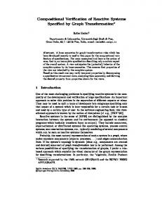
The most basic and most general part of our model are the definitions of asynchronous reactive systems with distributed scheduling. We consider sets of asynchronously communicating probabilistic state machines; we call such sets collections of machines. The left-hand side of Figure 1 sketches a collection of three machines connected via channels represented by solid arrows. To model asynchronous timing, messages sent between the machines stay on their respective channel until they are scheduled. Technically, each channel contains an additional machine called a buffer, which stores messages in transit. This is shown on the right-hand side of Figure 1. When M2 sends a message to M3 , this message is stored in the buffer. An incoming message at a clock channel for the buffer, represented by the dashed arrow, is interpreted as a number i, and the i-th message in the buffer is removed and output to M3 . Buffers need not be specified explicitly; a completion operator adds all necessary buffers to a collection of normal machines. As motivated in Section 1, we allow a machine that has been scheduled to schedule certain other machines itself. This is done by giving the machine the control over the clock channels 6

M1

M2

M3

M2 M3

Figure 1: A collection of three machines is shown on the left. Solid arrows represent channels. The dashed arrow depicts that M1 schedules messages on the channel from M2 to M3 . Each channel implicitly contains a buffer for storing messages in transit, shown on the right. of certain buffers. In Figure 1, the machine M1 can schedule messages sent from M2 to M3 , while the channels between M1 and M2 show procedure-call-style local interaction. Where one wants to express that an adversary schedules everything, one simply gives the adversary all the scheduling rights. Problems with purely adversarial scheduling were already noted in [40]; hence they schedule secure channels with uniform probability before adversary-chosen events. However, that introduces a certain amount of global synchrony. Furthermore, we do not require local scheduling for all secure channels; they may be blindly scheduled by the adversary (i.e., without even seeing if there are messages on the channel). For instance, this models cases where the adversary has a global influence on relative network speed. Probability spaces for runs are defined in detail for such collections of machines, as well as the view of a subset of the machines. These definitions are useful beyond the more securityspecific system classes considered later. Further, the Turing-machine realization and runtime considerations are defined in this generality. Security-specific structures are defined as collections of machines with distinguished service ports for the honest users, as explained in the introduction. Such structures are augmented by arbitrary machines H and A representing the honest users and the adversary, who can interact. We then speak of a configuration. For configurations, we also introduce specific families of executions corresponding to different security parameters for cryptographic aspects. In the presence of adversaries, the structure of correct machines running may not be the intended structure that the designer originally planned. For instance, some machines might have been corrupted; hence they are missing from the actual structure and the adversary took over their connections. We model this by defining a system as a set of possible actual structures. A system is typically derived automatically from an intended structure and a trust model. We define this for static and adaptive adversaries, arbitrary access structures limiting the corruption capabilities of an adversary, and different channel types. While one typically considers all basic channels insecure in a security protocol, secure or authentic channels are useful to model initialization phases, e.g., the assumption that a public-key infrastructure exists. In contrast to some formal methods which immediately abstract from cryptography, we cannot represent this by a fixed initial key set because we need probabilities over the key generation for security; further, it would not allow a polynomial number of keys to be chosen reactively. Reactive simulatability, our notion of secure refinement, is defined for individual structures and lifted entire systems. Two structures struc 1 and struc 2 can be compared if they have the same service ports, so that the same honest users can connect to them. In other words, they offer the same interface for the design of a larger system, so that either struc 1 or struc 2 can be plugged into that system. Now struc 1 is considered at least as secure as struc 2 , written struc 1 ≥ struc 2 , if whatever any adversary A1 can do to any honest user H in struc 1 , some adversary A2 can do 7

to the same H in struc 2 essentially with the same probability. More precisely, the families of views of H in these two configurations are indistinguishable. We present several flavors of this definition. Structure struc 1 typically represents a real distributed cryptographic primitive or protocol, while struc 2 is a specification in terms of one joint deterministic machine. This gives us the desired rigorous link between real cryptographic systems and abstractions suitable for automated theorem provers and model checkers.

3

Notation

n Let Bool := {true, false}. For an arbitrary set A, let P(A) denote its powerset. Further, S let An ∗ denote the set of sequences over A with index set I = {1, . . . , n} for n ∈ N0 , A := n∈N0 A , and A∞ the set of sequences over A with index set I = N. We write a sequence over A with index set I as S = (Si )i∈I , where ∀i ∈ I : Si ∈ A. Let ◦ denote sequence concatenation, and () the empty sequence. For a sequence S ∈ A∗ ∪ A∞ we define the following notation:

• For a function f : A → A′ , let f (S) apply f to each element of S, retaining the order. • For a predicate pred : A → Bool , let (Si ∈ S | pred (Si )) denote the subsequence of S containing those elements Si of S with pred (Si ) = true, retaining the order. • Let size(S) denote the length of S, i.e., size(S) := |I|. • For l ∈ N0 , let S⌈l denote the l-element prefix of S, and S[l] the l-th element of S with the convention that S[l] = ǫ if size(S) < l. In the following, we assume that a finite alphabet Σ ⊇ {0, 1} is given, where ∼, !, ?,↔ ,⊳ 6∈ Σ. Then Σ∗ denotes the strings over Σ. Let ǫ be the empty string and Σ+ := Σ∗ \ {ǫ}. All notation for sequences can be used for strings, such as ◦ for string concatenation, but ◦ is often omitted. For representing natural numbers and sequences of strings as strings, we assume bijective functions nat : Σ∗ → N with the convention nat(1) = 1 and ι : (Σ∗ )∗ → Σ∗ . We assume that standard operations are efficiently (polynomial-time) computable in these encodings; concretely we need this for inverting the function ι, for appending an element to a sequence of strings, and for retrieving and removing the nat(u)-th element from a sequence of strings. For an arbitrary set A let Prob(A) denote the set of all finite probability distributions over A. For a probability distribution D over A, the probability of a predicate pred : A → Bool is written PrD (pred ). If x is a random variable over A with distribution D, we also write PrD (pred (x)). In both cases we omit D if it is clear from the context. We write := for deterministic and ← for probabilistic assignment. The latter means that for a function f : X → Prob(Y ), we write y ← f (x) to denote that y is chosen according to the distribution f (x). For such a function f we write y := f (x) if there exists y ′ ∈ Y with Prf (x) (y ′ ) = 1. If the function f is clear from the context, we also write x →p y for Prf (x) (y) = p, and → for →1 . Further, we sometimes treat f (x) as a random variable instead of a distribution, e.g., by writing Pr(f (x) = y) for Prf (x) (y).

4

Asynchronous Reactive Systems

In this section, we define our model of interacting probabilistic machines with distributed scheduling and with computational realizations.

8

n !

Sending machine

n!

Scheduler for buffer ~ n

n ?

n ?

~ Buffer n n ! n?

Receiving machine

Figure 2: Ports and buffers.

4.1

Ports

Machines can exchange messages with each other via ports. Intuitively, a port is a possible attachment point for a channel when a machine of Figure 1 is considered in isolation. As in many other models, channels in collections of machines are specified implicitly by naming conventions on the ports; hence we define port names carefully. Figure 2 gives an overview of the naming scheme; it can be seen as a yet more detailed view of the right-hand side of Figure 1. Definition 4.1 (Ports) Let P := Σ+ × {ǫ, ↔ , ⊳ } × {!, ?}. Then p ∈ P is called a port. For p = (n, l, d) ∈ P, we call name(p) := n its name, label(p) := l its label, and dir(p) := d its direction. 3 In the following we usually write (n, l, d) as nld, i.e., as string concatenation. This is possible without ambiguity, since the mapping ϕ : P → Σ+ ◦ {ǫ, ↔ , ⊳ } ◦ {!, ?} with ϕ((n, l, d)) := nld is bijective because of the precondition !, ?,↔ ,⊳ 6∈ Σ. The name of a port serves as an identifier and will later be used to define which ports are connected to each other. The direction of a port determines whether it is a port where inputs occur or where outputs are made. Inspired by the CSP [33] notation, this is represented by the symbols ? and !, respectively. The label becomes clear in Definition 4.3. Definition 4.2 (In-Ports, Out-Ports) A port (n, l, d) is called an in-port or out-port iff d = ? or d = !, respectively. For a set P of ports let out(P ) := {p ∈ P | dir(p) = !} and in(P ) := {p ∈ P | dir(p) = ?}. For a sequence P of ports let out(P ) := (p ∈ P | dir(p) = !) and in(P ) := (p ∈ P | dir(p) = ?). 3 The label of a port determines the port’s role in the upcoming scheduling model. Roughly, ports p with label(p) ∈ {↔ ,⊳ } are used for scheduling whereas ports p with label(p) = ǫ are used for “usual” message transmission. Definition 4.3 A port p = (n, l, d) is called a simple port, buffer port or clock port iff l = ǫ, or ⊳ , respectively. 3

↔,

After introducing ports on their own, we now define the low-level complement of a port. This will later be the port which it connects to. Two connected ports have identical names and different directions. The relationship of their labels l and l′ is visible in Figure 2, i.e., l = l′ = ⊳ or {l, l′ } = {ǫ,↔ }. The remaining notation of Figure 2 is explained below. In particular, “Buffer e n” represents the network between the two simple ports n! and n?. If we are not interested in the network details then we regard the ports n! and n? as connected; thus we call them high-level complements of each other. 9

Definition 4.4 (Complement Operators) Let p = (n, l, d) be a port. a) The low-level complement pc of p is defined as pc := (n, l′ , d′ ) such that {d, d′ } = {!, ?}, and l = l′ = ⊳ or {l, l′ } = {ǫ,↔ }. b) If p is simple, the high-level complement pC of p is defined as pC := (n, l, d′ ) with {d, d′ } = {!, ?}. 3

4.2

Machines

After introducing ports, we now define machines. Our primary machine model is probabilistic state-transition machines, similar to probabilistic I/O automata as in [42, 57]. A machine has a sequence of ports, containing both in-ports and out-ports, and a set of states, comprising sets of initial and final states. If a machine is switched, it receives an input tuple at its input ports and performs its transition function yielding a new state and an output tuple in the deterministic case, or a finite distribution over the set of states and possible outputs in the probabilistic case. Furthermore, each machine has state-dependent bounds on the length of the inputs accepted at each port to enable flexible enforcement of runtime bounds, as motivated in Section 1. The parts of an input that are beyond the length bound are ignored. The value ∞ denotes that arbitrarily long inputs are accepted. Definition 4.5 (Machines) A machine is a tuple M = (name, Ports , States, δ, l, Ini , Fin) where • name ∈ Σ+ ◦ {∼, ǫ} is called the name of M, • Ports is a finite sequence of ports with pairwise distinct elements, • States ⊆ Σ∗ is called a set of states, • δ is called a probabilistic state-transition function and defined as follows: Let I := (Σ∗ )|in(Ports )| and O := (Σ∗ )|out(Ports )| denote the input set and output set of M, respectively. Then δ : States × I → Prob(States × O) with the following restrictions: – If I = (ǫ, . . . , ǫ), then δ(s, I) := (s, (ǫ, . . . , ǫ)) deterministically. – δ(s, I) = δ(s, I⌈l(s) ) for all I ∈ I, where (I⌈l(s) )i := Ii ⌈l(s)i for all i ∈ {1, . . . , |in(Ports)|}. (The parts of an input beyond the length bounds are ignored.) • l : States → (N0 ∪ {∞})|in(Ports )| is called a length function; we require l(s) = (0, . . . , 0) for all s ∈ Fin, • Ini , Fin ⊆ States are called the sets of initial and final states. 3

10

In the following, we write name M for the name of machine M, Ports M for its sequence of ports, States M , Ini M , Fin M for its respective sets of states, IM , OM for its input and output set, lM for its length function and δM for its transition function. The chosen representation makes the transition function δ independent of the port names; this enables port renaming in our proofs. The requirement for ǫ-inputs, i.e., the first restriction on δ, means that it does not matter if we switch a machine without inputs or not, i.e., there are no spontaneous transitions. The second restriction means that the part of each input beyond the current length bound for its port is ignored. In particular one can mask an input by a length bound 0 for a port. The restriction on l means that a machine ignores all inputs if it is in a final state, and hence it no longer switches. We will often need the port set of a machine instead of its port sequence. Port sets are easily extendible to a set of machines. Definition 4.6 (Port Set) The port set ports(M) of a machine S M is the set of ports in the ˆ ˆ sequence Ports M . For a set M of machines, let ports(M ) := M∈M 3 ˆ ports(M). In the following, we define three disjoint sets of machines. Membership in each set can be determined by the name and the ports of a machine. These sets do not serve as a partition of the set of all machines, but only machines contained in these sets matter in the following. This will become clear when we introduce how several machines interact and schedule each other. Simple machines only have simple ports and clock out-ports, and their names are contained in Σ+ . We do not make any restrictions on their internal behavior. Definition 4.7 (Simple Machines) A machine M is simple iff name M ∈ Σ+ and for all p = (n, l, d) ∈ ports(M) we have l = ǫ or (l, d) = (⊳ , !). 3 Similar to simple machines, master schedulers only have simple ports and clock out-ports, except that they have one special clock in-port clk⊳ ?, called the master-clock in-port. When we define the interaction of several machines, this port will be used to resolve situations where the interaction cannot proceed otherwise. A master scheduler must not make non-empty outputs in a transition that enters a final state. This will simplify the later definition that the entire interaction between machines stops if a master scheduler enters a final state. Definition 4.8 (Master Schedulers) A machine M is a master scheduler iff • name M ∈ Σ+ , • clk⊳ ? ∈ ports(M), • for all p = (n, l, d) ∈ ports(M) \ {clk⊳ ?}, we have l = ǫ or (l, d) = (⊳ , !), and • if Pr(δM (s, I) = (s′ , O)) > 0 with s′ ∈ Fin M and arbitrary s ∈ States M and I ∈ IM , then O = (ǫ, . . . , ǫ). 3 If a simple machine or a master scheduler M has an out-port n! or an in-port n? we say that M is the sending machine or receiving machine for n, as shown in Figure 2. As the third machine set, we define buffers. All buffers have the same predefined transition function. They model the asynchronous channels between other machines, and will later be inserted between two ports n! and n? as shown in Figure 2. More precisely, for each port name 11

n, we define a buffer denoted as e n with three ports n⊳ ?, n↔ ?, and n↔ !. When a value is input ↔ at n ?, the transition function of the buffer appends this value to an internal queue over Σ∗ . An input u 6= ǫ at n⊳ ? is interpreted as a natural number, captured by the function nat, and the nat(u)-th element of the internal queue is removed and output at n↔ !. If there are less than nat(u) elements, the output is ǫ. As the two inputs never occur together in the upcoming run algorithm, we define that the buffer only evaluates its first non-empty input. Since the states have to be a subset of Σ∗ by Definition 4.5, we embed the queue into Σ∗ using the embedding function ι for sequences (see Section 3). Definition 4.9 (Buffers) For every n ∈ Σ+ we define a machine e n called a buffer: e n := (n∼, (n⊳ ?, n↔ ?, n↔ !), States en , δen , len , Ini en , ∅)

with • Statesen := {ι(P ) | P ∈ (Σ∗ )∗ }, • Ini en := {ι(ǫ)}, • len (ι(P )) := (∞, ∞) for all ι(P ) ∈ States en , and

• δen (ι(P ), (u, v)) := (ι(P ′ ), (o)) deterministically as follows for (P1 , . . . , Psize(P ) ) := P: if u 6= ǫ then if nat(u) ≤ size(P ) then P ′ := (Pi ∈ P | i 6= nat(u)) o := Pnat(u) else P ′ := P and o = ǫ end if else if v 6= ǫ then P ′ := P ◦ (v) and o := ǫ else P ′ := P and o := ǫ end if 3 In the following, a machine with a tilde such as e n always means the unique buffer for n ∈ Σ+ according to Definition 4.9.

4.3

Computational Realization

For computational aspects, a machine M is regarded as implemented by a probabilistic interactive Turing machine as introduced in [31]. We need some refinements of this model. The main feature of interactive Turing machines is that they have communication tapes where one machine can write and one other machine can read. Thus we will use one communication tape to model each low-level connection. Probabilism is modeled by giving each Turing machine a read-only random tape containing an infinite sequence of independent, uniformly random bits. To make each Turing configuration finite, we can instead newly choose such a bit whenever a

12

cell of the random tape is first accessed. Each Turing machine has one distinguished work tape; it may or may not have further local tapes, which are initially empty. Our first refinement concerns how the heads move on communication tapes; our choice guarantees that a machine can ignore the ends of long messages as defined by the length functions in our I/O machine model, and nevertheless read the following message. This helps machines to guarantee certain runtimes without becoming vulnerable to denial-of-service attacks by an adversary sending a message longer than this runtime. This enables liveness properties, although those are not considered in this paper. The second refinement concerns restarts of machines in a multi-machine scenario. We guarantee that a switching step with only empty inputs is equivalent to no step at all, as in the I/O machine model. By a Turing machine whose heads recognize partner heads we mean a Turing machine whose transition function is based on its finite state and, for each of its heads, on the content of the cell under this head and a bit denoting whether another head is on the same cell. Definition 4.10 (Computational Realization of Machines) A probabilistic interactive Turing machine T is a probabilistic multi-tape Turing machine whose heads recognize partner heads. Tapes have a left boundary, and heads start on the left-most cell. T implements a machine M as defined in Definition 4.5 if the following holds. Let iM := |in(Ports M )|. We write “finite state” for a state of the finite control of T and “M-state” for an element of States M . a) T has a read-only tape for each in-port of M. Here the head never moves left, nor to the right of the other head on that tape. For each out-port of M, T has a write-only tape where the head never moves left of the other head on that tape. b) T has special finite states restartint (where “int” is similar to an interrupt vector) with int ∈ P({1, . . . , iM }) for waking up asynchronously with inputs at a certain set of ports, sleep denoting the end of an M-transition, and end for termination. Here restart∅ = sleep, i.e., T needs no time for “empty” transitions. c) T realizes δM (s, I) as follows for all s ∈ States M and I ∈ IM : Let T start in finite state restartint where int := {i | Ii ⌈lM (s)i 6= ǫ} = 6 ∅, with worktape content s, and with Ii on the i-th input tape from (including) T’s head to (excluding) the other head on this tape for all i. Let s′ be the worktape content in the next finite state sleep or end, and Oi the content of the i-th output tape from (including) the other head to (excluding) T’s head in that state. Then the pairs (s′ , O) are distributed according to δM (s, I), and the finite state is end iff s′ ∈ Fin M . 3 The main reason to introduce a Turing-machine realization of the machine model is to define complexity notions. The interesting question is how we handle the inputs on communication tapes in the complexity definition, in particular for the notion of polynomial time, which is the maximum complexity allowed to adversaries against typical cryptographic systems. One can imagine three degrees of an interactive machine being polynomial-time. The weakest would be that each M-transition only needs time polynomial in the current inputs and the current state, i.e., the current content of the local tapes. However, such a machine might double the size of its current state in each M-transition; then it would be allowed time exponential in an initial security parameter after a linear number of M-transitions. Hence we do not use this notion.

13

In the medium notion, which we call weakly polynomial-time, the runtime of the machine is polynomial in the overall length of its inputs, including the initial worktape content. Equivalently, the runtime for each M-transition is polynomial in the overall length of the inputs received so far. This makes the machine a permissible adversary when interacting with a cryptographic system which is in itself polynomially bounded. However, several weakly polynomialtime machines together (or even one with a self-connection) can become too powerful. E.g., each new output may be twice as long as the inputs so far. Then after a linear number of Mtransitions, these weakly polynomial-time machines are allowed time exponential in an initial security parameter. We nevertheless use weakly polynomial-time machines sometimes, because many functionalities are naturally weakly polynomial-time and not naturally polynomial-time in the following strong sense. However, one always has to keep in mind that this notion does not compose as we just saw. Finally, polynomial-time machines are those who only need time polynomial in their initial worktape content, independent of all inputs on communication tapes. A run of a probabilistic, interactive Turing machine is a valid sequence of configurations of T (defined as for other Turing machines), where the finite state end can only occur in the last configuration of the run. Definition 4.11 (Complexity of Machines) a) A probabilistic interactive Turing machine T is polynomial-time iff there exists a polynomial P such that all possible runs of T are of length at most P (k), where k is the length of the initial worktape content. b) T is called weakly polynomial-time iff there exists a polynomial P such that for every fixed initial worktape content and fixed contents of all input tapes with overall length k′ , all possible runs of T are of length at most P (k′ ). c) A machine M according to Definition 4.5 is (weakly) polynomial-time iff it has a realization as a (weakly) polynomial-time probabilistic interactive Turing machine. More generally, if we say without further qualification that T fulfills some complexity measure, we mean that all possible runs of the machine fulfill this measure as a function of the length k of the initial worktape content. 3 Besides the deterministic runtime bounds that we have defined and that we will use in the following, one could define bounds for the expected runtime.

4.4

Collections of Machines

After introducing individual machines, we now focus on collections of finitely many machines, with the intuition that these machines interact. Each machine in a collection must be uniquely determined by its name, and their port sets must be pairwise disjoint so that the naming conventions for low- and high-level complements will lead to well-defined one-to-one connections. Definition 4.12 (Collections) ˆ is a finite set of machines with pairwise different machine names, pairwise a) A collection C disjoint port sets, and where each machine is a simple machine, a master scheduler, or a buffer.

14

b) A collection is called (weakly) polynomial-time iff all its non-buffer machines are (weakly) polynomial-time. ˆ and n⊳ ! ∈ ports(M) then we call M the scheduler for buffer e ˆ , and we c) If e n, M ∈ C n in C ˆ omit “in C ” if it is clear from the context. 3 If a port and its low-level complement are both contained in the port set of the collection, they form a low-level connection; recall Definition 4.4. High-level connections for simple ports are defined similarly. If a port p is contained in the port set of the collection but its low-level complement is not, p is called free. Free ports will later be used to connect external, machines to the collection. For instance, a collection may consist of machines that execute a cryptographic protocol, and their free ports can be connected to users and an adversary. ˆ be a collection. Definition 4.13 (Connections) Let C ˆ ) then {p, pc } is called a low-level connection. The set gr(C ˆ ) := a) If p, pc ∈ ports(C c c ˆ )} is called the low-level connection graph of C ˆ. {{p, p } | p, p ∈ ports(C ˆ ) := ports(C ˆ ) \ ports(C ˆ )c we denote the free ports in C ˆ. b) By free(C ˆ ) then {p, pC } is called a high-level connection. The set Gr(C ˆ ) := c) If p, pC ∈ ports(C C C ˆ ˆ {{p, p } | p, p ∈ ports(C )} is called the high-level connection graph of C . 3 Given a collection of (usually simple) machines, we want to add buffers for all high-level conˆ. nections to model asynchronous timing. This is modeled by the completion of a collection C ˆ The completion is the union of C and buffers for all existing ports except the master-clock ˆ unchanged. A collection in-port. Note that completion leaves already existing buffers in C is called closed if the only free port of its completion is the master-clock in-port clk⊳ ?. This implies that a closed collection has precisely one master scheduler, identified by having the unique master-clock in-port. ˆ be a collection. Definition 4.14 (Closed Collection, Completion) Let C ˆ ] of C ˆ is defined as a) The completion [C ˆ ] := C ˆ ∪ {e ˆ ) \ {clk⊳ ?}}. [C n | ∃l, d : (n, l, d) ∈ ports(C ˆ is closed iff free([C ˆ ]) = {clk⊳ ?}, and C ˆ is complete iff [C ˆ] = C ˆ. b) C 3

4.5

Runs and their Probability Spaces

For a closed collection, we now define runs (in other terminologies executions or traces).

15

3. 1. I

O

~ o

MCS 4. ~ n

5. M’

Figure 3: Phases of the run algorithm. Informal Description We start with an informal description. Since the collection is closed, it contains a unique master scheduler X. Machines switch sequentially, i.e., we have exactly one active machine M at any time. If this machine has clock out-ports, it can select the next message to be delivered by scheduling a buffer via one of these clock out-ports. If a message exists at the respective position of the buffer’s internal queue, it is delivered by the buffer and the unique receiving machine is the next active machine. If M tries to schedule multiple messages, only one is taken, and if it schedules none or the message does not exist, the master scheduler X becomes active. Next we give a more precise, but still only semi-formal definition of runs. Runs and their probability spaces are defined inductively by the following algorithm for each tuple ˆ . The algorithm mainini ∈ ×M∈Cˆ Ini M of initial states of the machines of a collection C tains variables for the states of all machines of the collection and treats each port as a variable over Σ∗ , initialized with ǫ except for clk⊳ ? := 1. The algorithm further maintains a variable MCS (“current scheduler”) over machine names, initialized with MCS := X, for the name of the currently active simple machine or master scheduler, and a variable r for the resulting run, an initially empty list. The algorithm operates in five phases, which are illustrated in Figure 3. Probabilistic choices only occur in Phase 1. 1. Switch current scheduler: Switch the current machine MCS , i.e., set (s′ , O) ← δMCS (s, I) for its current state s and in-port values I. Then assign ǫ to all in-ports of MCS . 2. Termination: If X is in a final state, the run stops. (As X made no outputs in this case, this only prevents repeated master clock inputs.) 3. Store outputs: For each simple out-port o! of MCS with o! 6= ǫ, in their given order, switch buffer e o with input o↔ ? := o!. Then assign ǫ to all these ports o! and o↔ ?.

4. Clean up scheduling: If at least one clock out-port of MCS has a value 6= ǫ, let n⊳ ! denote the first such port and assign ǫ to the others. Otherwise let clk⊳ ? := 1 and MCS := X and go to Phase 1. 5. Deliver scheduled message: Switch e n with input n⊳ ? := n⊳ !, set n? := n↔ ! and then assign ǫ to all ports of e n and to n⊳ !. If n? = ǫ let clk⊳ ? := 1 and MCS := X. Else let MCS := M′ for the unique machine M′ with n? ∈ ports(M′ ). Go to Phase 1.

Whenever a machine (this may be a buffer) with name name M is switched from (s, I) to (s′ , O), we add a step (name M , s, I, s′ , O) to the run r with the following two restrictions. First, we cut each input according to the respective length function, i.e., we replace I by I ′ := I⌈lM (s) . 16

Secondly, we do not add the step to the run if I ′ = (ǫ, . . . , ǫ), i.e., if nothing happens in reality. This gives a family of probability distributions (run Cˆ ,ini ), one for each tuple ini of initial states ˆ of machines, we define the restriction of the machines of the collection. Moreover, for a set M ˆ switches. This is called the view of M ˆ . Similar of runs to those steps where a machine of M ˆ to runs, this gives a family of probability distributions (view Cˆ ,ini (M )), one for each tuple ini of initial states. Rigorous Definitions We now define the probability space of runs rigorously. Since the semi-formal description is sufficient to understand our subsequent results and the rigorous definitions are quite technical, this subsection can be skipped at first reading. We first define a global state space and a global transition function on these states. The global state space has five parts: the states of all machines of the collection, the current scheduler (currently active machine), a function assigning strings, the current values, to the ports of the collection, the current phase, and a subset of the out-port sequence of one machine for modeling the “for”-loop in the third phase of the informal algorithm. Additionally, the global state space contains a distinguished global final state sfin . ˆ be a complete, closed collection with Definition 4.15 (Global States of a Collection) Let C ˆ master scheduler X. Let PCˆ := {P | ∃M ∈ C : P ⊆ out(Ports M )} where ⊆ denotes the subsequence relation. ˆ is defined as • The set of global states of C ˆ

ˆ × (Σ∗ )ports(C ) × {1, . . . , 5} × P ˆ ∪ {sfin }. States Cˆ := ×M∈Cˆ StatesM × C C ˆ is defined as • The set of initial global states of C Ini Cˆ := ×M∈Cˆ Ini M × {X} × {f } × {1} × {()} ˆ ) \ {clk⊳ ?}. with f (clk⊳ ?) := 1 and f (p) := ǫ for p ∈ ports(C 3 On these global states, we define a global transition function. It reflects the informal run algorithm. ˆ be a complete, closed collection with masDefinition 4.16 (Global Transition Function) Let C ter scheduler X. We define the global transition function δCˆ : States Cˆ → Prob(States Cˆ ) by δCˆ (sfin ) := sfin and otherwise by the following rules: Phase 1: Switch current scheduler. ((sM )M∈Cˆ , MCS , f, 1, P ) →p ((s′M )M∈Cˆ , MCS , f ′ , 2, ()) where, with I := f (in(Ports MCS )) and O := f ′ (out(Ports MCS )), 17

(1)

• p = Pr(δMCS (sMCS , I) = (s′MCS , O)), ˆ \ {MCS }, and • sM = s′M for all M ∈ C ˆ ) \ ports(MCS ). • f ′ (in(Ports MCS )) = (ǫ)|in(Ports MCS )| and f ≡ f ′ on ports(C Phase 2: Termination. ((sM )M∈Cˆ , MCS , f, 2, P ) → sfin

if sX ∈ Fin X ;

(2)

((sM )M∈Cˆ , MCS , f, 2, P ) → ((sM )M∈Cˆ , MCS , f, 3, P ′ )

if sX 6∈ Fin X

(3)

where P ′ = (o! ∈ Ports MCS | o ∈ Σ+ ∧ f (o!) 6= ǫ). Phase 3: Store outputs. ((sM )M∈Cˆ , MCS , f, 3, ()) → ((sM )M∈Cˆ , MCS , f, 4, ()); ((sM )M∈Cˆ , MCS , f, 3, P ) → ((s′M )M∈Cˆ , MCS , f ′ , 3, P ′ )

(4) if P 6= ()

(5)

where there exists n ∈ Σ+ with • P = (n!) ◦ P ′ , • (se′n , (ǫ)) = δen (sen , (ǫ, f (n!))), ˆ \ {e n}, and • sM = s′M for all M ∈ C ˆ ) \ {n!}. • f ′ (n!) = ǫ and f ≡ f ′ on ports(C Phase 4: Clean up scheduling. Let Clks := (n⊳ ! ∈ Ports MCS | f (n⊳ !) 6= ǫ). Then ((sM )M∈Cˆ , MCS , f, 4, P ) → ((sM )M∈Cˆ , X, f ′ , 1, ())

if Clks = ()

(6)

if Clks 6= ()

(7)

ˆ ) \ {clk⊳ ?} and f ′ (clk⊳ ?) = 1, and where f ′ (p) = ǫ for all p ∈ ports(C ((sM )M∈Cˆ , MCS , f, 4, P ) → ((sM )M∈Cˆ , MCS , f ′ , 5, P ′ ) where • P ′ = (Clks[1]), and ˆ ) \ {Clks[1]c }. • f ′ (Clks[1]c ) = f (Clks[1]) and f ′ (p) = ǫ for all p ∈ ports(C Phase 5: Deliver scheduled message. if 6 ∃n ∈ Σ+ : P = (n⊳ !);

((sM )M∈Cˆ , MCS , f, 5, P ) → sfin ⊳

((sM )M∈Cˆ , MCS , f, 5, (n !)) →

((s′M )M∈Cˆ , M′CS , f ′ , 1, ())

(8) (9)

where, with u := f (n⊳ ?), there exists o ∈ Σ+ such that ˆ \ {e n}, • sM = s′M for all M ∈ C • (se′n , (o)) = δen (sen , (u, ǫ)),

and

ˆ)\ • either o = ǫ and M′CS = X and f ′ (clk⊳ ?) = 1 and f ′ (p) = ǫ for all p ∈ ports(C ⊳ {clk ?} 18

ˆ ) \ {n?}. • or o 6= ǫ and n? ∈ Ports M′CS and f ′ (n?) = o and f ′ (p) = ǫ for all p ∈ ports(C 3 Rule (8) has only been included to define the function δ on the entire state space States Cˆ as claimed at the beginning of the definition. It will not matter in the execution since the previous state has to be in Phase 4, and this ensures that P contains exactly one clock port. Similarly, the other rules make no assumptions about reachable states. Further, δ(s) is indeed an element of Prob(States Cˆ ) for every s ∈ States Cˆ : It is deterministic for all states s except those treated in Rule (1). For those, the claim follows immediately from the fact that δMCS (sMCS , I) is a finite distribution. Given the global probabilistic transition function δ, we now obtain probability distributions on sequences of global states by canonical constructions as for Markov chains. This even holds for infinite sequences by the theorem of Ionescu-Tulcea; see, e.g., Section V.1 of [50]. More precisely, we obtain one such probability distribution for every global initial state. Applying the theorem of Ionescu-Tulcea to our situation yields the following lemma. ˆ be a complete, closed collection, Lemma 4.1 (Probabilities of State Sequences) Let C and let an initial global state ini ∈ Ini Cˆ be given. For each set of fixed-length sequences States iCˆ with i ∈ N, we can define a finite probability distribution PStates Cˆ ,ini,i by Pr(S) =

i Y

Pr(δCˆ (Sj−1 ) = Sj )

j=2

for every sequence S = (S1 , . . . , Si ) over States Cˆ with S1 = ini , and Pr(S) = 0 otherwise. Further, for every sequence S ∈ States iCˆ , let Rect(S) denote the corresponding rectangle of ′ infinite sequences with this prefix, i.e., Rect(S) := {S ′ ∈ States ∞ ˆ | S ⌈i = S}. Then there exists C ∞ a unique probability distribution PStates Cˆ ,ini,∞ over States Cˆ whose value for every rectangle R := Rect(S) with S ∈ States iCˆ equals Pr(S), or more precisely, PrPStates Cˆ ,ini,∞ (R) := PrPStates Cˆ ,ini,i (S). We usually omit the indices “∞” and “i” of these distributions; this cannot lead to confusion. 2 Varying ini gives a family of probability distributions over States ∞ ˆ ; we write it C PStates Cˆ := (PStates Cˆ ,ini )ini∈Ini Cˆ . So far we have defined probabilities for sequences of entire global states. Each step in the runs introduced semi-formally above intuitively corresponds to the difference between two successive states: Moreover, only the switching of machines is considered in a run, i.e., the intermediate phases for termination checks and cleaning up scheduling are omitted, as well as the switching of machines with empty input (after application of the length function) because nothing happens then. We first define the set of possible steps, i.e., five-tuples containing the name of the currently switched machine M, its old state, its input tuple, its new state, and its output tuple. Further, we define an encoding of steps as strings for the sole purpose of defining overall lengths of potential runs.

19

Definition 4.17 (Steps) The set of steps is defined as Steps := (Σ+ ◦ {∼, ǫ}) × Σ∗ × (Σ∗ )∗ × Σ∗ × (Σ∗ )∗ . Let ιSteps : Steps → Σ+ denote a bijective function such that standard operations on Steps are For all r = (ri )i∈I ∈ Steps ∗ let len(r) := P efficiently computable in this encoding. ∞ let len(r) := ∞. 3 i∈I size(ιSteps (r)), and for r ∈ Steps Now we define a mapping that extracts a run from a step sequence. Our definition first extracts a sequence of one potential step from each pair of a global state and the next one. This first part maps intermediate phases to steps with empty input tuples, so that it is then sufficient to restrict the obtained sequence to the elements with a non-empty input tuple for getting rid of both the intermediate phases and of actual switching with empty inputs. When extracting a potential step, we mainly distinguish whether the current scheduler switches or a buffer; such a buffer is always indicated by the first element in the port sequence of outputs still to be handled, the fifth element of the global state. ˆ be a complete, closed collection. Then the run exDefinition 4.18 (Run Extraction) Let C ˆ is the function traction of C ∗ ∞ run Cˆ : States ∞ ˆ → Steps ∪ Steps C

ˆ except for its domain.) Let S = (Si )i∈N ∈ States ∞ defined as follows. (It is independent of C ˆ C with Si = sfin or Si = ((siM )M∈Cˆ , MiCS , f i , j i , P i ) for all i ∈ N. If i∗ := min{i ∈ N | si = sfin } exists, let I := {1, . . . , i∗ − 2}, otherwise I := N. We define a sequence pot step(S) = ′ ((ni , si , Ii , si , Oi ))i∈I as follows. (Thus we already omit the last termination check.) • If P i = () then, with M := MiCS , – ni := name M , – si := siM and s′i := si+1 M , and – if j i = 1 then Ii := f i (in(Ports M ))⌈lM (si ) and Oi := f i+1 (out(Ports M )), else Ii := (ǫ) and Oi := (ǫ). • If P i 6= (), let p := P i [1] and p ∈ ports(e n). Then – ni := n∼. – si := sein and s′i := seni+1 ,

– Ii := f i ((n⊳ ?, n↔ ?)) and Oi := f i+1 ((n↔ !)). Then run Cˆ (S ) := ((ni , si , Ii , s′i , Oi ) ∈ pot step(S) | Ii 6= (ǫ, . . . , ǫ)). let run Cˆ ,l denote the extraction of l-step prefixes of runs, run Cˆ ,l : States ∞ ˆ → C

[

For every number l ∈ N,

Steps i

i≤l

with run Cˆ ,l (S) := run Cˆ (S)⌈l .

3

20

The run extraction is a random variable on every probability space over States ∞ ˆ . For our C particular probability space, this induces a family run Cˆ = (run Cˆ ,ini )ini ∈Ini Cˆ of probability distributions over Steps ∗ ∪ Steps ∞ via Prrun Cˆ ,ini (r) := PrPStates Cˆ ,ini (run −1 ˆ (r)) C

for all r ∈ Steps ∗ ∪ Steps ∞ , where run −1 ˆ (r) is the set of pre-images of r. For a function C l : Ini Cˆ → N, this similarly gives a family of probability distributions run Cˆ ,l = (run Cˆ ,ini,l(ini) )ini ∈Ini Cˆ , each over

S

i≤l(ini) Steps

i

.

ˆ of machines in a collection. It is the restriction of We finally introduce the view of a set M ˆ . The extraction a run (a sequence of steps) to those steps whose machine name belongs to M ˆ anyway for similarity with the function is independent of the collection, but we index it with C run notation. ˆ be a complete, closed collection and M ˆ ⊆C ˆ . The view of M ˆ Definition 4.19 (Views) Let C ∗ ∞ ∗ ∞ ˆ ˆ in C is the function view Cˆ (M ) : Steps ∪ Steps → Steps ∪ Steps with ˆ )(r) := (si ∈ r | ∃M ∈ M ˆ : si [1] = name M ). view Cˆ (M ˆ ) denote the extraction of l-step prefixes of a view, i.e., For every number l ∈ N let view Cˆ ,l (M S i ˆ ) : Steps ∗ ∪ Steps ∞ → ˆ ˆ view Cˆ ,l (M 3 ˆ ,l (M )(r) := view C ˆ (M )(r)⌈l . i≤l Steps with view C ˆ = {M}, we write view ˆ (M) instead of view ˆ ({M ˆ }), and similar for l-step For a singleton M C C prefixes. Based on the family run Cˆ of probability distributions of runs, this induces a family of probability distributions ˆ ) = (view ˆ (M ˆ ))ini ∈Ini view Cˆ (M ˆ C ,ini C over Steps ∗ ∪ Steps ∞ . For a function l : Ini Cˆ → N, this similarly gives a family view Cˆ ,l = S (view Cˆ ,ini,l(ini) )ini ∈Ini Cˆ over i≤l(ini ) Steps i . Finally, we define sets of state-traces and of traces (or step-traces). Intuitively, they are the possible sequences of global states and of steps, respectively. More precisely, each finite prefix of such a sequence happens with positive probability. ˆ be a complete, closed collection and ini ∈ Ini ˆ Definition 4.20 (State-Trace, Trace) Let C C an initial global state. • The set of state-traces for ini is (S ⌈l ) > 0}. StateTrace Cˆ ,ini := {S ∈ States ∞ ˆ | ∀l ∈ N : PrPStates C ˆ ,ini,l C • The set of traces for ini is StepTrace Cˆ ,ini

:= {tr ∈ Steps ∗ | Prrun Cˆ ,ini (tr ) > 0} ∪

{tr ∈ Steps ∞ | ∀l ∈ N : Prrun Cˆ ,ini,l (tr ⌈l ) > 0}.

21

ˆ ⊆C ˆ for ini is • The set of possible views of a machine set M ˆ )(v ) > 0} ˆ ) := {v ∈ Steps ∗ | Prview (M ViewTrace Cˆ ,ini (M ˆ ,ini C ∪ Set StateTrace Cˆ := ˆ ) := S ViewTrace ˆ (M C

S

ˆ )(v ⌈l ) > 0}. {v ∈ Steps ∞ | ∀l ∈ N : Prview Cˆ ,ini,l (M

StateTrace Cˆ ,ini and Trace Cˆ ˆ ). ViewTrace ˆ (M

ini∈Ini C ˆ

ini∈Ini C ˆ

:=

S

ini∈Ini C ˆ

Trace Cˆ ,ini and

C ,ini

3

We conclude this section with two properties of state-traces and views. The first, technical ˆ , which only one states that whenever a non-buffer machine M is switched in a state-trace of C ˆ happens in Phase 1, there is at most one port p ∈ ports(C ) with a non-empty value, and it must fulfill p ∈ ports(M). ˆ be a complete, closed collection. Let S := Lemma 4.2 (Unique Inputs in Traces) Let C (Si )i∈N ∈ StateTraceCˆ with Si = sfin or Si = ((siM )M∈Cˆ , Mi , f i , j i , P i ) for all i. For all i ∈ N with Si 6= sfin : ˆ ) : (f i (p) 6= ǫ)) ⇒ (p ∈ ports(Mi ) ∧ ∀p′ ∈ ports(C ˆ ) \ {p} : (f i (p′ ) = ǫ)). (j i = 1 ∧ ∃p ∈ ports(C 2 Proof. For i = 1 this holds since S ∈ StateTrace Cˆ implies S1 ∈ Ini Cˆ and each element of Ini Cˆ fulfills the claim with p = clk⊳ !. Let now i > 1 and Si with j i = 1. Only two cases are possible for the previous state Si−1 . The case j i−1 = 4 and Mi = X fulfills the claim for p = clk⊳ ? ∈ ports(X), and the case j i−1 = 5 for p = n?. The second property shows that the views of polynomial-time machines are polynomially bounded, and so are runs of polynomial-time collections. ˆ ⊆ C ˆ be polynomial-time. For all Lemma 4.3 (Polynomial Views and Traces) Let M P ini = ((ini M )M∈Cˆ , X, f, 1, ()) ∈ Ini Cˆ let sizeM ˆ (ini ) := ˆ size(ini M ). Then there exM∈M ˆ ) we have ists a polynomial P such that for all ini ∈ Ini Cˆ and all v ∈ ViewTrace Cˆ ,ini (M len(v) ≤ P (sizeM ˆ (ini )). ˆ is polynomial-time, then there exists a polynomial P such that for If the entire collection C all ini ∈ Ini Cˆ and all r ∈ Trace Cˆ ,ini we have len(r) ≤ P (sizeCˆ (ini )). 2 Proof. By Definition 4.11, a polynomial-time machine M only makes a polynomial number of Turing steps, relative to the length size(ini M ) of its own input, which is smaller than the overall input size sizeM ˆ (ini ) of the considered machines. Consequently, M can only build up a polynomial-size state and outputs, and read a polynomial-size part of its inputs. Each step in the view requires at least one Turing step; hence there is also only a polynomial number of these steps. Further, only states, outputs, and read parts of the inputs are part of the steps (see Definitions 4.16 and 4.18). This proves the first statement. ˆ consists of the steps of its polynomial-time machines A run of a polynomial-time collection C and its buffers. Buffers are not polynomial-time, but weakly polynomial-time; this follows immediately from the assumption we made about the encoding ι of the internal queue. Each buffer obtains all its inputs from polynomial-time machines; hence its overall input is of polynomial length. Thus each buffer only makes a polynomial number of Turing steps. This yields an overall polynomial size of its steps as above. 22

5

Security-specific System Model

We now define specific collections for security purposes. We start with the definition of structures. Intuitively, these are the machines that execute a security protocol. Structures additionally have so-called service ports, which are a subset of the free ports of the completion of the collection. Roughly, service ports are those where a certain service of the structure is guaranteed. Typical examples of inputs at service ports are “send message m to participant id ” for a message transmission system or “pay amount x to participant id ” for a payment system. Concretely, service ports will later be used to connect a user machine to a structure. For cryptographic purposes, the initial state of all machines is typically a security parameter k in unary representation. Hence we require that such strings of 1s are valid initial states of all machines. ˆ , S ) where M ˆ Definition 5.1 (Structures and Service Ports) A structure is a pair struc = (M ∗ ˆ ˆ is a collection of simple machines with {1} ⊆ Ini M for all M ∈ M , and S ⊆ free([M ]). The set S is called service ports. 3 Forbidden ports for users of a structure are those that clash with port names of given machines and those that would link the user to a non-service port. ˆ , S ) let S ¯ ˆ := free([M ˆ ]) \ S . We call Definition 5.2 (Forbidden Ports) For a structure (M M ˆ , S ) := ports(M ˆ )∪S ¯ c the forbidden ports. 3 forb(M ˆ M A system is a set of structures. The idea behind systems, as motivated in Section 2, is that there may be different actual structures depending on the set of actually malicious participants. Typical derivations of systems from one explicitly defined intended structure and a trust model will be discussed in Section 7. Definition 5.3 (Systems) A system Sys is a set of structures. It is (weakly) polynomial-time ˆ of all its structures are (weakly) polynomial-time. iff the machine collections M 3 A structure can be complemented to a configuration by adding a user machine and an adversary machine (or user and adversary for short). The user is restricted to connecting to the service ports. The adversary closes the collection, i.e., it connects to the remaining service ports, to ¯ ˆ of the collection, and to the free ports of the user. Thus, user and the other free ports S M adversary can interact, e.g., for modeling active attacks. Definition 5.4 (Configurations) ˆ , S ) is a tuple conf = (M ˆ , S , H, A) where a) A configuration of a structure (M ˆ , S ) = ∅, – H is a machine called user without forbidden ports, i.e., ports(H) ∩ forb(M ∗ and with {1} ⊆ Ini H , – A is machine called adversary with {1}∗ ⊆ Ini A , ˆ := [M ˆ ∪ {H, A}] is a closed collection. – and the completion C ˆ , S ) is written Conf(M ˆ , S ). The set of configurations of b) The set of configurations of (M ˆ ˆ , S ). (M , S ) with polynomial-time user H and adversary A is written Conf poly (M c) S The

set

of configurations of a system Sys S is defined as Conf(Sys) ˆ ˆ ˆ ,S )∈Sys Conf(M , S ), and similarly Confpoly (Sys) := ˆ ,S )∈Sys Conf poly (M , S ). (M (M 23

:=

H

H

S

S

M1

M2

A1

A2

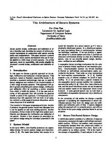
Figure 4: Example of reactive simulatability. The view of H is compared. Whatever an adversary A1 can achieve in the configuration on the left-hand side, another A2 can achieve the same in the configuration on the right-hand side. We omit the index “poly” from Confpoly (Sys) if it is clear from the context.

3

In cryptographic applications, all machines typically start with the same security parameter. Hence we make a global constraint on the valid global initial states in the family of runs of a configuration that the security parameters are equal. ˆ , S , H, A) be a configuration Definition 5.5 (Runs and Views of Configurations) Let conf = (M k ˆ := [M ˆ ∪ {H, A}]. We define Ini conf := {((1 ) ˆ and C ˆ , (X, f, 1, ())) | k ∈ M∈M ∪{H,A} ◦ (ι(ǫ))e n∈C N} ⊆ Ini Cˆ with X and f as in Definition 4.15. Then we define the family of probability distributions of runs of the configuration as run conf := (run Cˆ ,ini )ini ∈Ini conf ˆ′⊆C ˆ the family of probability distributions of views similarly and for all sets M ˆ ′ ) := (view ˆ (M ˆ ′ ))ini ∈Ini , view Cˆ (M conf C ,ini and analogously for l-step prefixes. Furthermore, we identify Ini conf with N and thus write run conf ,k etc. for the individual probability distributions in the families. 3

6

Reactive Simulatability

The definition of one structure securely implementing another one is based on the concept of simulatability. Our definition is the first such definition for an asynchronous reactive setting and is hence called reactive simulatability. As explained in Section 2, reactive simulatability ˆ 1, S ) essentially means that whatever might happen to an honest user in a real structure (M ˆ 2 , S ). More precisely, for every configuration conf 1 ∈ can also happen in an ideal structure (M ˆ ˆ 2 , S ) with the same user yielding Conf(M1 , S ), there exists a configuration conf 2 ∈ Conf(M indistinguishable views for this user in both configurations. A typical situation is illustrated in Figure 4. We need notions that functions are small; hence we define corresponding function classes. Definition 6.1 (Small functions) a) The class NEGL of negligible functions contains all functions s : N → R≥0 that decrease faster than the inverse of every polynomial, i.e., for all positive polynomials Q ∃k0 ∀k > 1 . k0 : s(k) < Q(k)

24

b) A set SMALL of functions N → R≥0 is a class of small functions if it is closed under addition, and with a function g also contains every function g′ : N → R≥0 with g′ ≤ g. 3 Typical classes of small functions are EXPSMALL, which contains all functions bounded by Q(k) · 2−k for a polynomial Q, and the larger class NEGL. Simulatability is based on indistinguishability of views; hence we repeat the definition of indistinguishability, essentially from [63]. Definition 6.2 (Indistinguishability) Two families (vark )k∈N and (var′k )k∈N of probability distributions (or random variables) on common domains (Dk )k∈N are a) perfectly indistinguishable (“ =”) iff ∀k ∈ N : vark = var′ k . b) statistically indistinguishable (“≈SMALL ”) for a class SMALL of small functions iff the distributions are discrete and their statistical distances, as a function of k, are small, i.e., (∆stat (vark , var′k ))k∈N := (

1 X |Pr(vark = d) − Pr(var′k = d)|)k∈N ∈ SMALL. 2 d∈Dk

c) computationally indistinguishable (“≈poly ”) iff for every algorithm Dis (the distinguisher) that is probabilistic polynomial-time in its first input, (|Pr(Dis(1k , vark ) = 1) − Pr(Dis(1k , var′k ) = 1)|)k∈N ∈ NEGL. (Intuitively, Dis, given the security parameter and an element chosen according to either vark or var′k , tries to guess which distribution the element came from.) We write ≈ if we want to treat all cases together.

3

We now present the reactive simulatability definition. One technical problem is that a user might ˆ 1 , S ), but in a configuration legitimately connect to the service ports in a configuration of (M ˆ of (M2 , S ) the same user might have forbidden ports. This is excluded by considering suitable configurations only. ˆ 1 , S ) and (M ˆ 2 , S ) be strucDefinition 6.3 (Suitable Configurations for Structures) Let (M ˆ ˆ 1, S ) ⊆ tures with the same set of service ports. The set of suitable configurations Conf M2 (M ˆ M ˆ 1 , S ) is defined by (M ˆ 1 , S , H, A) ∈ Conf 2 (M ˆ 1 , S ) iff ports(H) ∩ forb(M ˆ 2 , S ) = ∅. Conf(M ˆ2 ˆ2 ˆ M ˆ 1 , S ) := Conf M (M1 , S ) ∩ The set of polynomial-time suitable configurations is Conf poly (M ˆ Conf poly (M1 , S ). 3 As we have three different notions of indistinguishability, our reactive simulatability definition also comes in three flavors. Further, we distinguish the general simulatability as sketched so far and a stronger universal version where one adversary A2 must be able to work for all users. ˆ 1 , S ) and (M ˆ 2, S ) Definition 6.4 (Reactive Simulatability for Structures) Let structures (M with identical sets of service ports be given.

25

ˆ 1 , S ) ≥perf ˆ ˆ a) (M sec (M2 , S ), spoken perfectly at least as secure as (M2 , S ), iff for every conˆ M ˆ 1 , S , H, A1 ) ∈ Conf 2 (M ˆ 1 , S ), there exists a configuration conf 2 = figuration conf 1 = (M ˆ ˆ (M2 , S , H, A2 ) ∈ Conf(M2 , S ) (with the same H) such that view conf 1 (H) = view conf 2 (H). ˆ 2 , S ), spoken statistically at least as secure as, for a class SMALL of ˆ 1 , S ) ≥SMALL (M b) (M sec ˆ2 ˆ ˆ 1 , S , H, A1 ) ∈ Conf M small functions iff for every configuration conf 1 = (M (M1 , S ), there ˆ ˆ exists a configuration conf 2 = (M2 , S , H, A2 ) ∈ Conf(M2 , S ) (with the same H) such that view conf 1 ,l (H) ≈SMALL view conf 2 ,l (H) for all polynomials l, i.e., if all families of l-step prefixes of the views are statistically indistinguishability. ˆ ˆ 1 , S ) ≥poly c) (M sec (M2 , S ), spoken computationally at least as secure as, iff for every conˆ2 ˆ ˆ 1 , S , H, A1 ) ∈ Conf M figuration conf 1 = (M poly (M1 , S ), there exists a configuration conf 2 = ˆ 2 , S , H, A2 ) ∈ Conf poly (M ˆ 2 , S ) (with the same H) such that (M view conf 1 (H) ≈poly view conf 2 (H). In all three cases, we speak of universal simulatability if A2 in conf 2 does not depend on H uni,perf ˆ 1 , S , and A1 ), and we use the notation ≥sec etc. for this. In all cases, we call (only on M conf 2 an indistinguishable configuration for conf 1 . 3 There is also a notion of blackbox simulatability, where the adversary A2 consists of a fixed part, called simulator, using A1 as a blackbox submachine. However, its rigorous definition needs the notion of machine combination, which we postpone to the successor paper dealing with composition. If one can simply set A2 := A1 , we also say that the structures are indistinguishable; this corresponds to the definition in [39]. Where the difference between the types of security is irrelevant, we simply write ≥sec , and we omit the index sec if it is clear from the context. Remark 6.1. Adding a free adversary out-port in the comparison (like the guessing-outputs used to define semantic security of encryption systems in [30]) does not make the definition stricter: Any such out-port can be connected to an in-port added to the honest user with sufficiently large length bounds. H does not react on inputs at this new in-port, but nevertheless it is included in the view of H, i.e., in the comparison. A rigorous proof can be found in [4]. ◦ The definition of reactive simulatability can be lifted from structures to systems Sys 1 and Sys 2 by comparing their respective structures. However, we do not want to compare a structure of Sys 1 with arbitrary structures of Sys 2 , but only with certain “suitable” ones. What suitable means in a concrete situation can be defined by a mapping f from Sys 1 to the powerset of Sys 2 . The mapping f is called valid if it maps structures with the same set of service ports, so that the same user can connect. For many systems there is only one possible mapping that meets this requirement, because the service ports of the structures correspond to one-to-one to different sets of non-corrupted machines. This mapping is then called canonical.

26

Definition 6.5 (Valid Mappings) Let Sys 1 and Sys 2 be two systems. a) A valid mapping between Sys 1 and Sys 2 is a function f : Sys 1 → P(Sys 2 ) \ ∅ with S1 = S2 ˆ 1 , S1 ) ∈ Sys 1 and (M ˆ 2 , S2 ) ∈ f ((M ˆ 1 , S1 )). Structures (M ˆ 2 , S2 ) with (M ˆ 2 , S2 ) ∈ for all (M ˆ ˆ f ((M1 , S1 )) are called corresponding structures of (M1 , S1 ). b) If there is only one valid mapping f between Sys 1 and Sys 2 , it is called the canonical mapping. 3 Remark 6.2. In the synchronous model in [55], we allow more general users and valid mappings. The stronger requirements here simplify the presentation and are sufficient for all cryptographic examples we considered. Its report version contains non-cryptographic examples with S1 6= S2 . ◦ An example of a system that contains different structures with the same service ports, so that a non-canonical mapping is needed, is a protocol with a semi-trusted third-party machine T which needs no user interface because its behavior is fully prescribed by the protocol, and where different properties can be achieved depending on whether T is correct or not. Before we introduce reactive simulatability for systems, we define suitable configurations for entire systems with respect to a valid mapping. Definition 6.6 (Suitable Configurations for Systems) Let Sys 1 , Sys 2 be systems, and f a valid mapping between Sys 1 and Sys 2 . The set of suitable configurations Conf f (Sys 1 ) ⊆ Conf(Sys 1 ) ˆ ˆ 1 , S ) for all (M ˆ 2 , S ) ∈ f ((M ˆ 1 , S )). The set is defined by conf ∈ Conf f (Sys 1 ) iff conf ∈ Conf M2 (M f of polynomial-time suitable configurations is Conf poly (Sys 1 ) := Conf f (Sys 1 ) ∩ Confpoly (Sys 1 ). 3 Definition 6.7 (Reactive Simulatability for Systems) Let Sys 1 and Sys 2 be systems, and f a valid mapping between Sys 1 and Sys 2 . Let x ∈ {perf, poly} or x = SMALL for a class SMALL of small functions, and let x′ ∈ {x, (uni, x)}. f,x ′ ˆ 1 , S ) ∈ Sys 1 there exists with (M ˆ 2 , S ) ∈ f ((M ˆ 1 , S )) Then Sys 1 ≥sec Sys 2 if for every (M such that ′ ˆ 1 , S ) ≥xsec ˆ 2 , S ). (M (M Depending on the value of x, we say that Sys 1 is perfectly / statistically / computationally at least as secure as Sys 2 . We omit the indices f , x′ , and sec if they are clear from the context. 3 We conclude this section with two technical lemmas capturing an equivalent definition of the forbidden ports of a structure and additional results on valid mappings and suitable configurations, which is useful in proofs. Recall that Definition 5.4 excludes users that would connect to the forbidden ports of a configuration. The following lemma establishes an equivalent condition. ˆ , S ) be a structure. Then for all machines H, ports(H) ∩ Lemma 6.1 (Users) Let (M ˆ , S ) = ∅ is equivalent to ports(H) ∩ ports(M ˆ ) = ∅ (1) and ports(H)c ∩ ports([M ˆ ]) ⊆ S (2). forb(M 2

27

ˆ ) := ports(C ˆ ) \ free(C ˆ ) for every collection C ˆ . Clearly inner(C ˆ )c = inner(C ˆ ). Proof. Let inner(C c ˆ The condition on the left-hand side is equivalent to (1) and ports(H) ∩ (free([M ]) \ S ) = ∅ (3). ˆ ]) ⊆ S . It remains to be shown that ports(H)c ∩ inner([M ˆ ]) = ∅. Now (3) ⇔ ports(H)c ∩ free([M ˆ ˆ This is equivalent to ports(H) ∩ inner([M ]) = ∅. Now ports([M ]) only contains additional buffer ˆ ). Hence (1) even implies ports(H)∩ports([M ˆ ]) = ports and clock in-ports compared with ports(M ∅. The following lemma shows that the ports of a structure that users are intended to use, i.e., the complement of the service ports, are not at the same time forbidden. Moreover, it shows that a non-suitable configuration can be transformed into a suitable one via port renaming such that this renaming does not affect the view of the user. This means that the restriction to suitable configurations in the definition of reactive simulatability is without loss of generality. ˆ 1 , S ) and (M ˆ 2 , S ) be Lemma 6.2 (Valid Mappings and Suitable Configurations) Let (M structures. ˆ 1 , S ) = ∅. a) Then S c ∩ forb(M ˆ2 ˆ ˆ 1 , S , H, A1 ) ∈ Conf(M ˆ 1 , S ) \ Conf M b) For every conf 1 = (M (M1 , S ), there is a configuration ˆ2 ˆ M ˆ conf f,1 = (M1 , S , Hf , Af,1 ) ∈ Conf (M1 , S ) such that view conf f,1 (Hf ) = view conf 1 (H).

2 ˆ , S ) = ports(M ˆ 1 ) ∪ (free([M ˆ 1 ]) \ S )c . The part S c ∩ Proof. For Part a) recall that forb(M ˆ 1 ]) \ S )c = ∅ is clear, and S c ∩ ports(M ˆ 1 ) = ∅ follows from S ⊆ free([M ˆ 1 ]). (free([M ˆ 2, S ) a For Part b), we want to construct Hf by giving each port p = nld ∈ ports(H) ∩ forb(M new name. Since runs and views do not depend on port names, cf. Definition 4.5, they remain the same if we consistently rename all other ports q (at most five) with name(q) = n. The ˆ 1 , S , Hf , Af,1 ) if no renamed port belongs to M ˆ 1 . Assume new collection is a configuration (M ′ ′ c ˆ ˆ ˆ 1 ]). that q = nl d ∈ ports(M1 ) is such a renamed port, then e n ∈ [M1 ] and hence p ∈ ports([M c ˆ 2 , S ) implies p 6∈ Now Lemma 6.1 implies p ∈ S , hence Part a) applied to the structure (M ˆ forb(M2 , S ), in contradiction to the original condition on p.

7

Special Cases for Cryptographic Purposes

After defining structures, systems and reactive simulatability generally in the previous sections, we now define some specializations of the general model, which are of special importance for cryptographic purposes. We define standard cryptographic systems which are derived from an intended structure and a trust model. Intuitively, an intended structure represents a benign world, where each machine is correct. A trust model is then used to designate the potentially malicious sets of machines, i.e., machines which are considered to come under control of the adversary. Moreover, it classifies the “security” of each connection between machines of the structure, e.g., that a channel keeps messages authentic, but not secret. This is depicted in Figure 5: the left-hand side shows an intended structure consisting of three machines; the righthand side shows a possible derivation where machine M3 is malicious and channels have been modified. Cryptographic systems come in two flavors, depending on how the adversary takes control over certain machines. If malicious machines are malicious from the beginning, we call the system a static standard cryptographic system. If the adversary may corrupt machines during 28

User

Chosen-message attacks etc.

H

H

clk ?

S Machines

M1

M2

M1

M3

M2

M3

Adversary

A Figure 5: Derivation of one possible structure from an intended structure. The structures are the black parts. p!

p?

pd ! p!

p?

a

pd ? Adversary

p!

p?

p!

pa ? pa ! p? p?

i

Adversary

Figure 6: Channel modifications for authenticated and insecure channels. the protocol executions, depending on the knowledge that he has already collected, we speak of an adaptive standard cryptographic system.

7.1

Trust Models and Intended Structures

We start with the definition of trust models for a structure. Trust models consist of two parts: an access structure and a channel model. Access structures will later be used to denote the possible sets of correct machines in an intended structure. Access structures have to be closed under insertion, i.e., with every such set, every larger set is contained as well. Definition 7.1 (Access Structure) Let A be an arbitrary set. Then ACC ⊆ P(A) is called an access structure for A iff (B ∈ ACC ∧ C ∈ P(A) ∧ B ⊆ C ) ⇒ C ∈ ACC. 3 Typical examples of access structures are threshold structures ACC t,n := {H ⊆ A | |H| ≥ t} with t ≤ n. A channel model for a structure classifies each internal high-level connection as secure (private and authentic), authenticated (only authentic), or insecure (neither private nor authentic), represented as elements of the set {s, a, i}. What this means will become clear in Section 7.2. ˆ ∗ , S ∗ ) is a mapping Definition 7.2 (Channel Model) A channel model for a structure (M ˆ ∗ ) → {s, a, i}. χ : Gr(M 3 ˆ , S ) is a pair (ACC, χ) where Definition 7.3 (Trust Model) A trust model for a structure (M ˆ ˆ , S ). ACC is an access structure for M , and χ is a channel model for (M 3 29

We proceed with the definition of intended structures, i.e., structures a designer of a security protocol would typically design. An intended structure is a structure that is benign in the sense that it does not offer any free simple ports for the adversary. Moreover, we demand that a machine of a structure may only schedule those connections for which it owns the corresponding input or output port, i.e., it does not intend to schedule users and adversaries. We distinguish three different kinds of intended structures, depending on how the channels between the system and the user are clocked. We call the structure localized if every output is clocked by the outputting machine itself. Structures of this kind are typically used as local submachines that can be clocked by the overall protocol and then immediately deliver a result. If the adversary clocks the communication between the structure and the user, we call the structure stand-alone. Finally, if the user and the system have to fetch the outputs of the other, we call the structure fetching. Remark 7.1. We could as well distinguish channels from the user to the system and vice versa, e.g., to define that users schedule their outputs and fetch their inputs. This would give nine different combinations. Modifying the upcoming definition of intended structures in such a way is trivial. ◦ The derivation of the remaining structures based on the intended structure will rely on modifying the connections in an adequate way, e.g., by duplicating output ports that output on authentic channels so that one output port is connected as usual and the duplicated port is connected to the adversary. Hence derived structures need an extended set of possible port names. Moreover, we will need a distinguished state and distinguished ports to model adaptive corruptions of machines. Technically, we therefore parameterize intended structures by an additional alphabet Γ ( Σ with |Γ| = |Σ| − 2 and a state scorr , and we restrict port names in the intended structure to Γ+ and possible states to Σ∗ \ {scorr }. ˆ ∗ , S ∗ ) is called an intended structure for Definition 7.4 (Intended Structure) A structure (M ∗ scorr ∈ Σ and Γ ⊂ Σ with |Γ| = |Σ| − 2 iff ˆ ∗ are simple, name(p) ∈ Γ+ for all p ∈ ports(M ˆ ∗ ), and scorr 6∈ States M for all • all M ∈ M ∗ ˆ M∈M , ˆ ∗ : (n⊳ ! ∈ ports(M) ⇒ (n? ∈ ports(M)) ∨ (n! ∈ ports(M))), and • for all M ∈ M ˆ ∗ ]) | label(pc ) = ǫ}. • it has the following properties. Let S ′ := {p ∈ free([M – The structure is called localized iff ˆ ∗ ])c }. S ∗ = S ′ ∪ {n⊳ ? | n! ∈ free([M ˆ ∗ holds: and the following condition on the port set of M ˆ ∗ ])c ⇒ n⊳ ! ∈ ports(M ˆ ∗) n? ∈ free([M

ˆ ∗ schedules its outputs to the user #M

– The structure is called stand-alone iff S ∗ = S ′ and ˆ ∗ ])c ⇒ n⊳ ! 6∈ ports(M ˆ ∗) # M ˆ ∗ does not schedule any connection (n, ǫ, d) ∈ free([M ˆ∗ # between the user and M

30

– The structure is called fetching iff ˆ ∗ ])c } S ∗ = S ′ ∪ {n⊳ ? | n? ∈ free([M ˆ ∗ holds: and the following condition on the port set of M ˆ ∗ ])c ⇒ n⊳ ! ∈ ports(M ˆ ∗) n! ∈ free([M

ˆ ∗ schedules the inputs from the user #M 3

7.2

Standard Static Cryptographic Systems

Standard static cryptographic systems are derived from an intended structure and a trust model as follows. Each system contains one structure for each element of the considered access structure, i.e., for each set H of potential correct machines. The channel model is taken into account as follows. Intuitively, we change the connections such that the adversary receives messages sent on authenticated and insecure channels, and we enable him to arbitrarily modify messages sent on insecure channels. This is modeled as depicted in Figure 6 for authenticated and insecure channels; secure channels remain unchanged. Authenticated channels are modeled by additional out-ports pd ! where outputs at p! are duplicated. The port pd ! remains free; hence the adversary can connect to it. Insecure channels are modeled by renaming the input port. This breaks the existing connection and places the adversary in between. Moreover, if p? belongs to a correct machine and p! does not, we also rename p? into pa ? so that all inputs from the adversary have superscript a. By applying these changes to a machine M, we get a modified machine MH,χ . Formally, let {a, d} := Σ \ Γ. Then we define two mappings ϕa and ϕd that assign each port p = (n, l, d) with n ∈ Γ+ ports (an, l, d) and (dn, l, d) respectively. We write pa and pd instead of ϕa (p) and ϕd (p). We now define the derivation of static cryptographic systems from a given intended structure and a trust model rigorously. Similar to the definition of runs, the semi-formal description given above is sufficient to understand our subsequent results, so the following technical definition can be skipped at first reading. ˆ ∗ , S ∗ ) be an inDefinition 7.5 (Derivation of Standard Static Cryptographic Systems) Let (M ˆ ∗ , S ∗ ). tended structure for a state scorr and a set Γ, and let (ACC, χ) be a trust model for (M Then the corresponding cryptographic system with static adversary ˆ ∗ , S ∗ ), (ACC, χ)) Sys = StanStat ((M ˆ H , SH ) | H ∈ ACC} where for all H ∈ ACC: is Sys := {(M • SH := S ∗ ∩ free([H]). ˆ H := {MH,χ |M ∈ H}, where • M MH,χ = (nameM , Ports MH,χ , States M , δMH,χ , lM , Ini M , Fin M ) is defined as follows: – The sequence Ports MH,χ is derived by the following algorithm. 31

Ports MH,χ := (). for p ∈ Ports M (in the given order) do if c := {p, pC } ∈ Gr(H) ∧ χ(c) = a ∧ dir(p) = ! then Ports MH,χ := Ports MH,χ ◦ (p, pd ) else if c := {p, pC } ∈ Gr(H) ∧ χ(c) = i ∧ dir(p) = ? then Ports MH,χ := Ports MH,χ ◦ (pa ) else if c := {p, pC } 6∈ Gr(H) ∧ dir(p) = ? then Ports MH,χ := Ports MH,χ ◦ (pa ) else Ports MH,χ := Ports MH,χ ◦ (p) end if end for – Let s, s′ ∈ States M , I ∈ (Σ∗ )|in(ports(M))| , O1 ∈ (Σ∗ )|out(ports(M))| and O2 ∈ (Σ∗ )|out(ports(MH,χ ))| . Then Pr(δMH,χ (s, I) = (s′ , O2 )) := Pr(δM (s, I) = (s′ , O1 )) if O2 is derived from O1 by the following algorithm, and zero otherwise.2 i := 1 for j := 1, . . . , |out(ports(MH,χ ))| do if (out(Ports MH,χ ))j = pd for a port p then 2 Oj2 := Oj−1 else Oj2 := Oi1 i := i + 1 end if end for 3

7.3

Standard Cryptographic Systems with Adaptive Adversaries

Standard static cryptographic systems as defined in the previous section are based on the intuition that corrupted machines are corrupted right from the start, e.g., they belong to untrusted owners. In adaptive (or dynamic) adversary models the set of corrupted machines can increase over time, e.g., because there is a “master adversary” who has to hack into machines in order to corrupt them [15, 21]. Adaptive adversary models are more powerful than static ones, i.e., there are examples of systems secure against static adversaries that are insecure against adaptive adversaries who can corrupt the same number of machines [21]. For a given intended structure and a channel model, the corresponding cryptographic system with adaptive adversary has only one structure. Similar to the derivation of static cryptographic systems from an intended structure, we define the derivation of a machine Mcorr,χ from each machine M. This derivation is used to grant the adversary the possibility to corrupt machines during the global execution. This is modeled by giving Mcorr,χ a corruption port corruptMcorr,χ ?, which is used for corruption requests, and two new ports cor outMcorr,χ !, cor inMcorr,χ ? for communication with the adversary after corruption. We assume that these ports must neither occur in an intended structure nor after port renaming as defined for the static case; this can be achieved by encoding the names of these ports into Σ+ \ ({ǫ, a, d} ◦ Γ+ ) where Σ = Γ ∪ {a, d}. 2 Note that |in(ports(M))| = |in(ports(MH,χ ))| by definition; hence I is also a valid input tuple for the machine MH,χ .

32

The corruption port must connect to the service ports. Upon a non-empty input at the corruption port, Mcorr sends its current state to the adversary via cor outMcorr,χ !, and from now on acts transparently, i.e., every input (I1 , . . . , Is ) is translated into the output ι(I1 , . . . , Is ) at cor outMcorr,χ !, and every input (b) at cor inMcorr,χ ? is first decomposed as (O1 , . . . , Ot ) := ι−1 (b) and then output at the respective output ports. ˆ ∗ , S ∗ ) be an Definition 7.7 (Derivation of Standard Adaptive Cryptographic Systems) Let (M ˆ ∗ , S ∗ ). intended structure for a state scorr and a set Γ, and let χ be a channel model χ for (M Then the corresponding cryptographic system with adaptive adversary ˆ ∗ , S ∗ ), χ) Sys = StanAdap((M ˆ , S )} where is Sys := {(M ˆ ∗ }. • S := S ∗ ∪ {corruptM ↔ ? | M ∈ M ˆ := {Mcorr,χ | M ∈ M ˆ ∗ }, where Mcorr,χ is derived from M with H = M ˆ as follows: Let • M MH,χ be the machine defined in the static case (Definition 7.5). Then Mcorr,χ = (nameM , Ports Mcorr,χ , States Mcorr,χ , δMcorr,χ , lMcorr,χ , Ini M , Fin M ) is defined as follows: – Ports Mcorr,χ := Ports MH,χ ◦ (corruptMcorr,χ ?, cor outMcorr,χ !, cor inMcorr,χ ?). – States Mcorr,χ := States M ∪ {scorr }. – lMcorr,χ (s) := lM (s) ◦ (1, 0) for s ∈ States M , and lMcorr,χ (scorr ) := (∞, . . . , ∞) ◦ (0, ∞). – Let I =: I ′ ◦(a, b). If (a, b) = (ǫ, ǫ) and s 6= scorr , then δMcorr,χ (s, I) := δMH,χ (s, I ′ )◦(ǫ). Otherwise δMcorr,χ (s, I) := (s′ , O) with O := O′ ◦ (o) is defined as follows: if a 6= ǫ and s 6= scorr then s′ := scorr , o := s, and O′ := (ǫ, . . . , ǫ) else if s = scorr then o := ι(I) if b = ǫ then O′ = (ǫ, . . . , ǫ) else (o1 , . . . , ot ) := ι−1 (b) and t′ := size(out(Ports MH,χ )) Oj′ := oj for j = 1, . . . , min(t, t′ ) and Oj′ := ǫ for j = t + 1, . . . , t′ end if end if 3 Note that Mcorr,χ is not polynomial-time. Explicitly bounding the number of bits read in a corrupted state independent of the adversary does not capture our intuition of a machine that acts transparently for any adversary, and an explicit bound would severely limit the adversary’s capabilities. The fundamental problem is that transparent machines are by definition not polynomial-time but only weakly polynomial-time. Several extensions are possible: One may extend the corruption responses to two classes of storage, an erasable and a non-erasable one, e.g., to model the different vulnerability of 33

session keys and long-term keys. This means to refine the state spaces of each machine as a Cartesian product. In- and outputs would be treated like erasable storage. One can also model non-binary corruption requests, e.g., stop requests and requests to corrupt different classes of storage. To model proactive systems [51], one needs repair requests in addition to corruption requests, and appropriate repair responses, e.g., returning to an initial state with only a certain class of storage still intact.

8

Summary

We have presented a rigorous model for secure reactive systems with cryptographic parts in asynchronous networks. Common types of cryptographic systems and their trust models were expressed as special cases of this model, in particular systems with static or adaptive adversaries and with different types of underlying channels. We have defined reactive simulatability as a notion of refinement that retains not only integrity properties but also confidentiality. As design principles based on this model, we propose to keep specifications of cryptographic systems abstract, i.e., free of all implementation details and deterministic unless the desired functionality is probabilistic by nature, e.g., a common coin-flipping protocol. This allows the cryptographically verified abstractions to be used as building blocks for systems that can be subjected to formal verification. Suitable abstractions sometimes have to explicitly include tolerable imperfections of systems, e.g., leakage of the length of encrypted messages or abilities of the adversary to disrupt protocol runs. In subsequent work, we already showed multiple desired properties of reactive simulatability, in particular composition and property-preservation theorems. We also proved several building blocks like secure message transmission and a Dolev-Yaostyle cryptographic library with nested operations. Moreover, we demonstrated the applicability of formal methods over our model by small examples.

Acknowledgment We thank Anupam Datta, Martin Hirt, Dennis Hofheinz, Paul Karger, Ralf K¨ usters, John Mitchell, J¨ orn M¨ uller-Quade, Andre Scedrov, Matthias Schunter, Victor Shoup, Michael Steiner, Rainer Steinwandt, Dominique Unruh and an anonymous reviewer for interesting discussions. In particular, joint work with Matthias on examples of synchronous reactive systems also influenced this asynchronous model, and so did joint work with Michael on liveness and adaptiveness. Dennis, J¨orn, Rainer, and Dominique pointed out some subtle problems. The anonymous reviewer provided enough motivation for making the model much more rigorous than it was before. This work was partially supported by the European IST Project MAFTIA. However, it represents the view of the authors. The MAFTIA project was partially funded by the European Commission and the Swiss Federal Office for Education and Science (BBW).

References [1] M. Abadi and A. D. Gordon. A calculus for cryptographic protocols: The spi calculus. Information and Computation, 148(1):1–70, 1999.

34

[2] M. Abadi and J. J¨ urjens. Formal eavesdropping and its computational interpretation. In Proc. 4th International Symposium on Theoretical Aspects of Computer Software (TACS), pages 82–94, 2001. [3] M. Abadi and P. Rogaway. Reconciling two views of cryptography: The computational soundness of formal encryption. In Proc. 1st IFIP International Conference on Theoretical Computer Science, volume 1872 of Lecture Notes in Computer Science, pages 3–22. Springer, 2000. [4] M. Backes. Cryptographically Sound Analysis of Security Protocols. PhD thesis, Universit¨at des Saarlandes, 2002. http://www.zurich.ibm.com/~mbc/papers/PhDthesis.ps.gz. [5] M. Backes and D. Hofheinz. How to break and repair a universally composable signature functionality. IACR Cryptology ePrint Archive 2003/240, Nov. 2003. http://eprint. iacr.org/. [6] M. Backes and C. Jacobi. Cryptographically sound and machine-assisted verification of security protocols. In Proc. 20th Annual Symposium on Theoretical Aspects of Computer Science (STACS), volume 2607 of Lecture Notes in Computer Science, pages 675–686. Springer, 2003. [7] M. Backes, C. Jacobi, and B. Pfitzmann. Deriving cryptographically sound implementations using composition and formally verified bisimulation. In Proc. 11th Symposium on Formal Methods Europe (FME 2002), volume 2391 of Lecture Notes in Computer Science, pages 310–329. Springer, 2002. [8] M. Backes and B. Pfitzmann. Computational probabilistic non-interference. In Proc. 7th European Symposium on Research in Computer Security (ESORICS), volume 2502 of Lecture Notes in Computer Science, pages 1–23. Springer, 2002. [9] M. Backes and B. Pfitzmann. A cryptographically sound security proof of the NeedhamSchroeder-Lowe public-key protocol. In Proc. 23rd Conference on Foundations of Software Technology and Theoretical Computer Science (FSTTCS), 2003. [10] M. Backes and B. Pfitzmann. Intransitive non-interference for cryptographic purposes. In Proc. 24th IEEE Symposium on Security & Privacy, pages 140–152, 2003. [11] M. Backes, B. Pfitzmann, M. Steiner, and M. Waidner. Polynomial fairness and liveness. In Proc. 15th IEEE Computer Security Foundations Workshop (CSFW), pages 160–174, 2002. [12] M. Backes, B. Pfitzmann, and M. Waidner. A composable cryptographic library with nested operations (extended abstract). In Proc. 10th ACM Conference on Computer and Communications Security, pages 220–230, 2003. Full version in IACR Cryptology ePrint Archive 2003/015, Jan. 2003, http://eprint.iacr.org/. [13] M. Backes, B. Pfitzmann, and M. Waidner. A general composition theorem for secure reactive systems. In Proc. 1st Theory of Cryptography Conference (TCC), 2004. To appear. [14] D. Beaver. Secure multiparty protocols and zero knowledge proof systems tolerating a faulty minority. Journal of Cryptology, 4(2):75–122, 1991.

35

[15] D. Beaver and S. Haber. Cryptographic protocols provably secure against dynamic adversaries. In Advances in Cryptology: EUROCRYPT ’92, volume 658 of Lecture Notes in Computer Science, pages 307–323. Springer, 1992. [16] M. Bellare, R. Canetti, and H. Krawczyk. A modular approach to the design and analysis of authentication and key exchange protocols. In Proc. 30th Annual ACM Symposium on Theory of Computing (STOC), pages 419–428, 1998. [17] M. Bellare and P. Rogaway. Entity authentication and key distribution. In Advances in Cryptology: CRYPTO ’93, volume 773 of Lecture Notes in Computer Science, pages 232–249. Springer, 1994. [18] M. Blum and S. Micali. How to generate cryptographically strong sequences of pseudorandom bits. SIAM Journal on Computing, 13(4):850–864, 1984. [19] M. Burrows, M. Abadi, and R. Needham. A logic for authentication. Technical Report 39, SRC DIGITAL, 1990. [20] R. Canetti. Studies in secure multiparty computation and applications. Department of Computer Science and Applied Mathematics, The Weizmann Institute of Science, June 1995, revised March 1996, 1995. [21] R. Canetti. Security and composition of multiparty cryptographic protocols. Journal of Cryptology, 3(1):143–202, 2000. [22] R. Canetti. Universally composable security: A new paradigm for cryptographic protocols. In Proc. 42nd IEEE Symposium on Foundations of Computer Science (FOCS), pages 136– 145, 2001. Extended version in Cryptology ePrint Archive, Report 2000/67, http:// eprint.iacr.org/. [23] R. Canetti and S. Goldwasser. An efficient threshold public key cryptosystem secure against adaptive chosen ciphertext attack. In Advances in Cryptology: EUROCRYPT ’99, volume 1592 of Lecture Notes in Computer Science, pages 90–106. Springer, 1999. [24] Y. Desmedt and K. Kurosawa. How to break a practical mix and design a new one. In Advances in Cryptology: EUROCRYPT 2000, volume 1807 of Lecture Notes in Computer Science, pages 557–572. Springer, 2000. [25] D. Dolev and A. C. Yao. On the security of public key protocols. IEEE Transactions on Information Theory, 29(2):198–208, 1983. [26] R. Gennaro and S. Micali. Verifiable secret sharing as secure computation. In Advances in Cryptology: EUROCRYPT ’95, volume 921 of Lecture Notes in Computer Science, pages 168–182. Springer, 1995. [27] O. Goldreich. Secure multi-party computation. Department of Computer Science and Applied Mathematics, The Weizmann Institute of Science, June 1998, revised Version 1.4 October 2002, 1998. http://www.wisdom.weizmann.ac.il/users/oded/pp.htm. [28] O. Goldreich, S. Micali, and A. Wigderson. How to play any mental game – or – a completeness theorem for protocols with honest majority. In Proc. 19th Annual ACM Symposium on Theory of Computing (STOC), pages 218–229, 1987. 36

[29] S. Goldwasser and L. Levin. Fair computation of general functions in presence of immoral majority. In Advances in Cryptology: CRYPTO ’90, volume 537 of Lecture Notes in Computer Science, pages 77–93. Springer, 1990. [30] S. Goldwasser and S. Micali. Probabilistic encryption. Journal of Computer and System Sciences, 28:270–299, 1984. [31] S. Goldwasser, S. Micali, and C. Rackoff. The knowledge complexity of interactive proof systems. SIAM Journal on Computing, 18(1):186–207, 1989. [32] M. Hirt and U. Maurer. Player simulation and general adversary structures in perfect multiparty computation. Journal of Cryptology, 13(1):31–60, 2000. [33] C. A. R. Hoare. Communicating Sequential Processes. International Series in Computer Science, Prentice Hall, Hemel Hempstead, 1985. [34] D. Hofheinz, J. M¨ uller-Quade, and R. Steinwandt. Initiator-resilient universally composable key exchange. In Proc. 8th European Symposium on Research in Computer Security (ESORICS), volume 2808 of Lecture Notes in Computer Science, pages 61–84. Springer, 2003. [35] R. Impagliazzo and B. M. Kapron. Logics for reasoning about cryptographic constructions. In Proc. 44th IEEE Symposium on Foundations of Computer Science (FOCS), pages 372– 381, 2003. [36] R. Kemmerer. Analyzing encryption protocols using formal verification techniques. IEEE Journal on Selected Areas in Communications, 7(4):448–457, 1989. [37] R. Kemmerer, C. Meadows, and J. Millen. Three systems for cryptographic protocol analysis. Journal of Cryptology, 7(2):79–130, 1994. [38] P. Laud. Semantics and program analysis of computationally secure information flow. In Proc. 10th European Symposium on Programming (ESOP), pages 77–91, 2001. [39] P. Lincoln, J. Mitchell, M. Mitchell, and A. Scedrov. A probabilistic poly-time framework for protocol analysis. In Proc. 5th ACM Conference on Computer and Communications Security, pages 112–121, 1998. [40] P. Lincoln, J. Mitchell, M. Mitchell, and A. Scedrov. Probabilistic polynomial-time equivalence and security analysis. In Proc. 8th Symposium on Formal Methods Europe (FME 1999), volume 1708 of Lecture Notes in Computer Science, pages 776–793. Springer, 1999. [41] G. Lowe. Breaking and fixing the Needham-Schroeder public-key protocol using FDR. In Proc. 2nd International Conference on Tools and Algorithms for the Construction and Analysis of Systems (TACAS), volume 1055 of Lecture Notes in Computer Science, pages 147–166. Springer, 1996. [42] N. Lynch. Distributed Algorithms. Morgan Kaufmann Publishers, San Francisco, 1996. [43] N. Lynch. I/O automaton models and proofs for shared-key communication systems. In Proc. 12th IEEE Computer Security Foundations Workshop (CSFW), pages 14–29, 1999. [44] C. Meadows. Using narrowing in the analysis of key management protocols. In Proc. 10th IEEE Symposium on Security & Privacy, pages 138–147, 1989. 37

[45] C. Meadows. Formal verification of cryptographic protocols: A survey. In Proc. ASIACRYPT ’94, volume 917 of Lecture Notes in Computer Science, pages 135–150. Springer, 1994. [46] S. Micali and P. Rogaway. Secure computation. In Advances in Cryptology: CRYPTO ’91, volume 576 of Lecture Notes in Computer Science, pages 392–404. Springer, 1991. [47] J. K. Millen. The interrogator: A tool for cryptographic protocol security. In Proc. 5th IEEE Symposium on Security & Privacy, pages 134–141, 1984. [48] J. Mitchell, M. Mitchell, and A. Scedrov. A linguistic characterization of bounded oracle computation and probabilistic polynomial time. In Proc. 39th IEEE Symposium on Foundations of Computer Science (FOCS), pages 725–733, 1998. [49] J. Mitchell, M. Mitchell, A. Scedrov, and V. Teague. A probabilistic polynominal-time process calculus for analysis of cryptographic protocols (preliminary report). Electronic Notes in Theoretical Computer Science, 47:1–31, 2001. [50] J. Neveu. Mathematical Foundations of the Calculus of Probability. Holden-Day, 1965. [51] R. Ostrovsky and M. Yung. How to withstand mobile virus attacks. In Proc. 10th ACM Symposium on Principles of Distributed Computing (PODC), pages 51–59, 1991. [52] L. Paulson. The inductive approach to verifying cryptographic protocols. Journal of Cryptology, 6(1):85–128, 1998. [53] B. Pfitzmann and M. Waidner. How to break and repair a “provably secure” untraceable payment system. In Advances in Cryptology: CRYPTO ’91, volume 576 of Lecture Notes in Computer Science, pages 338–350. Springer, 1992. [54] B. Pfitzmann and M. Waidner. A general framework for formal notions of “secure” systems. Research Report 11/94, University of Hildesheim, Apr. 1994. http://www.semper.org/ sirene/lit/abstr94.html#PfWa_94. [55] B. Pfitzmann and M. Waidner. Composition and integrity preservation of secure reactive systems. In Proc. 7th ACM Conference on Computer and Communications Security, pages 245–254, 2000. Extended version (with Matthias Schunter) IBM Research Report RZ 3206, May 2000, http://www.semper.org/sirene/publ/PfSW1_00ReactSimulIBM.ps.gz. [56] B. Pfitzmann and M. Waidner. A model for asynchronous reactive systems and its application to secure message transmission. In Proc. 22nd IEEE Symposium on Security & Privacy, pages 184–200, 2001. Extended version in Cryptology ePrint Archive, Report 2000/066, http://eprint.iacr.org/. [57] R. Segala and N. Lynch. Probabilistic simulation for probabilistic processes. In Proc. 5th International Conference on Concurrency Theory (CONCUR), volume 836 of Lecture Notes in Computer Science, pages 481–497. Springer, 1994. [58] R. Segala and N. Lynch. Probabilistic simulation for probabilistic processes. Nordic Journal of Computing, 2(2):250–273, 1995. [59] M. Steiner. Secure Group Key Agreement. PhD thesis, Universit¨at des Saarlandes, 2002. http://www.semper.org/sirene/publ/Stei_02.thesis-final.pdf. 38

[60] F. J. Thayer Fabrega, J. C. Herzog, and J. D. Guttman. Strand spaces: Why is a security protocol correct? In Proc. 19th IEEE Symposium on Security & Privacy, pages 160–171, 1998. [61] S.-H. Wu, S. A. Smolka, and E. W. Stark. Composition and behaviors of probabilistic I/O automata. Theoretical Computer Science, 176(1–2):1–38, 1997. [62] A. C. Yao. Protocols for secure computations. In Proc. 23rd IEEE Symposium on Foundations of Computer Science (FOCS), pages 160–164, 1982. [63] A. C. Yao. Theory and applications of trapdoor functions. In Proc. 23rd IEEE Symposium on Foundations of Computer Science (FOCS), pages 80–91, 1982.

39