Secure Multi-Constrained QoS Reliable Routing ...

Secure Multi-Constrained QoS Reliable Routing Algorithm for Vehicular Ad hoc Networks (VANETs)

Mahmoud Hashem Eiza College of Engineering, Design and Physical Sciences Brunel University London

A thesis submitted for the degree of Doctor of Philosophy September 2014

I dedicate this work to every mother in my home country, Syria Your patience and devotion are an inspiration

ii

Acknowledgements I am grateful to many individuals for their care and support given during my doctoral studies. First and foremost, I would like to express my profound gratitude to Prof Qiang Ni and Dr Thomas Owens, my supervisors, for their enthusiastic encouragement, insightful advice, and invaluable suggestions. This work would not have been possible without them and their tremendous willingness to anticipate. I also would like to thank all those in Brunel University London, the college’s Department of Electronic & Computer Engineering (ECE). Finally, my special thanks should also go to my father, mother, sisters, and friends since they always have loved me, believed in me, and encouraged me throughout my studies. Last but not least, a final acknowledgement goes to my dearest friend Maria for her support, understanding, and encouragement.

iii

Abstract Vehicular Ad hoc Networks (VANETs) are a particular form of wireless network made by vehicles communicating among themselves and with roadside base stations. A wide range of services has been developed for VANETs ranging from safety to infotainment applications. A key requirement for such services is that they are offered with Quality of Service (QoS) guarantees in terms of service reliability and availability. Furthermore, due to the openness of VANET’s wireless channels to both internal and external attacks, the application of security mechanisms is mandatory to protect the offered QoS guarantees. QoS routing plays an essential role in identifying routes that meet the QoS requirements of the offered service over VANETs. However, searching for feasible routes subject to multiple QoS constraints is in general an NP-hard problem. Moreover, routing reliability needs to be given special attention as communication links frequently break in VANETs. To date, most existing QoS routing algorithms are designed for stable networks without considering the security of the routing process. Therefore, they are not suitable for applications in VANETs. In this thesis, the above issues are addressed firstly by developing a link reliability model based on the topological and mathematical properties of vehicular movements and velocities. Evolving graph theory is then utilised to model the VANET communication graph and integrate the developed link reliability model into it. Based on the resulting extended evolving graph model, the most reliable route in the network is picked. Secondly, the situational awareness model is applied to the developed reliable routing process because picking the most reliable route does not guarantee reliable transmission. Therefore, a situation-aware reliable multipath routing algorithm for VANETs is proposed. Thirdly, the Ant Colony Optimisation (ACO) technique is employed to propose an Ant-based multi-constrained QoS (AMCQ) routing algorithm for VANETs. AMCQ is designed to give significant advantages to the implementation of security mechanisms that are intended to protect the QoS routing process. Finally, a novel set of security procedures is proposed to defend the routing process against external and internal threats. Simulation results demonstrate that high levels of QoS can be still guaranteed by AMCQ even when the security procedures are applied.

iv

Supporting Publications Journals and Magazines 1. M.H. Eiza and Q. Ni, "An Evolving Graph-Based Reliable Routing Scheme for VANETs," IEEE Transactions on Vehicular Technology, vol. 62, no. 4, pp. 1493-1504, May 2013. DOI: 10.1109/TVT.2013.2244625 2. M.H. Eiza, Q. Ni, T. Owens and G. Min, "Investigation of Routing Reliability of

Vehicular

Ad

Hoc

Networks," EURASIP

Journal

on

Wireless

Communications and Networking, vol. 2013, no. 179, pp. 1-15, July 2013. DOI: 10.1186/1687-1499-2013-1791 3. M.H. Eiza, T. Owens and Q. Ni, "Secure and Robust Multi-Constrained QoS aware Routing Algorithm for VANETs," IEEE Transactions on Dependable and Secure Computing, Jan 2015. DOI: 10.1109/TDSC.2014.2382602

Conference Papers 1. M.H. Eiza and Q. Ni, "A Reliability-Based Routing Scheme for Vehicular Ad Hoc Networks (VANETs) on Highways," Presented at the IEEE 11th International Conference on Trust, Security and Privacy in Computing and Communications (TrustCom), Liverpool, UK, pp. 1578-1585, June 2012. DOI: 10.1109/TrustCom.2012.53

Presentations 1. M.H. Eiza and T. Owens, "On Reliable Routing as a Situational Awareness Aspect in Vehicular Ad Hoc Networks (VANETs)," in Intelligence and the Cyber Environment, Part of the Seminar Series on Emergent Issues in 21st Century Intelligence, Brunel University London, May 17-18, 2013.

1

This paper is designated as highly accessed

v

Contents CONTENTS ....................................................................................................................... VI LIST OF FIGURES .............................................................................................................. X LIST OF TABLES ............................................................................................................. XII LIST OF SYMBOLS ........................................................................................................XIV LIST OF ACRONYMS ................................................................................................... XIX 1

INTRODUCTION ......................................................................................................... 1 1.1 RESEARCH CHALLENGE ............................................................................................................... 2 1.2 AIM AND OBJECTIVES.................................................................................................................... 3 1.3 MAJOR CONTRIBUTIONS .............................................................................................................. 5 1.3.1 Link Reliability Model for VANETs on Highways.......................................................... 5 1.3.2 VANET-oriented Evolving Graph Model for Reliable Routing in VANETs....... 6 1.3.3 Situation-aware Reliable Routing Algorithm for VANETs ......................................... 7 1.3.4 Secure Ant-based Multi-Constrained QoS Routing Algorithm for VANETs ..... 8 1.4 THESIS OUTLINE .............................................................................................................................. 9

2

FUNDAMENTALS OF VANETS ............................................................................. 10 2.1 VANETS ARCHITECTURE AND FEATURES ........................................................................ 10 2.1.1 Vehicular Communication Paradigms ............................................................................... 10 2.1.2 Special Features and Challenges ........................................................................................... 12 2.1.3 Current Trends and Promising Applications.................................................................. 14 2.2 VEHICULAR TRAFFIC FLOW MODELLING .......................................................................... 15 2.2.1 Classification of Vehicular Traffic Flow Models ............................................................ 15 2.2.2 Vehicular Mobility Models ..................................................................................................... 17 2.2.3 The Highway Mobility Model ................................................................................................ 20 2.3 ROUTING IN VEHICULAR AD HOC NETWORKS ................................................................ 26 2.3.1 Taxonomy of VANET Routing Protocols ......................................................................... 26 2.3.2 Multi-Constrained QoS Routing in VANETs ............................................................... 30 2.4 SECURITY CHALLENGES OF ROBUST ROUTING IN VANETS ...................................... 34 2.4.1 General Security Challenges and Requirements of VANETs .................................. 34 2.4.2 Security Threats against the Routing Process ................................................................ 37 2.5 SUMMARY ....................................................................................................................................... 40

3

RELIABLE ROUTING ALGORITHM FOR VANETS ......................................... 41 3.1 STATE OF THE ART....................................................................................................................... 41 3.2 CHALLENGES OF RELIABLE ROUTING IN VANETS ........................................................ 43 3.3 VEHICULAR RELIABILITY MODEL.......................................................................................... 43 3.3.1 Link Reliability Model ............................................................................................................... 44

vi

3.3.2 Route Reliability Definition .................................................................................................... 46 3.4 RELIABILITY-BASED ROUTING PROTOCOL FOR VANETS (AODV-R).................... 47 3.4.1 Route Discovery Process in AODV-R ............................................................................... 49 3.4.2 Performance Evaluation of AODV-R................................................................................. 51 3.4.3 Simulation Results...................................................................................................................... 54 3.5 VANET-ORIENTED EVOLVING GRAPH MODEL .............................................................. 60 3.5.1 Motivation ...................................................................................................................................... 60 3.5.2 Basis of the Evolving Graph Theoretical Model ............................................................. 61 3.5.3 VANET-oriented Evolving Graph (VoEG)...................................................................... 62 3.5.4 Constructing and Maintaining the VoEG Model ......................................................... 65 3.6 EVOLVING GRAPH-BASED RELIABLE ROUTING PROTOCOL FOR VANETS........... 65 3.6.1 The Evolving Graph Dijkstra’s Algorithm (EG-Dijkstra)......................................... 66 3.6.2 The Computational Complexity of EG-Dijkstra’s algorithm .................................... 68 3.6.3 Route Discovery Process in EG-RAODV ........................................................................ 69 3.6.4 Performance Evaluation of EG-RAODV .......................................................................... 71 3.6.5 Simulation Results...................................................................................................................... 72 3.7 SUMMARY ....................................................................................................................................... 82 4

SITUATION-AWARE RELIABLE ROUTING ALGORITHM FOR VANETS 83 4.1 STATE OF THE ART....................................................................................................................... 83 4.2 BASIS OF THE SITUATIONAL AWARENESS MODEL.......................................................... 87 4.3 SITUATIONAL AWARENESS MODEL FOR RELIABLE ROUTING IN VANETS.......... 88 4.4 SITUATION-AWARE RELIABLE (SAR) ROUTING ALGORITHM ................................... 91 4.4.1 Problem Formulation ................................................................................................................. 91 4.4.2 Routing Control Messages & Routing Table in SAR.................................................. 92 4.4.3 Route Discovery Process in SAR Routing Algorithm................................................. 94 4.4.4 Route Maintenance Process in SAR Routing Algorithm ....................................... 100 4.4.5 Performance Evaluation of SAR ........................................................................................ 101 4.4.6 Simulation Results................................................................................................................... 102 4.5 SUMMARY ..................................................................................................................................... 111

5

ANT-BASED MULTI-CONSTRAINED QOS ROUTING ALGORITHM FOR

VANETS ............................................................................................................................ 112 5.1 RELATED WORK ......................................................................................................................... 112 5.2 MCQ ROUTING PROBLEM FORMULATION ...................................................................... 116 5.3 ACO RULES FOR MCQ ROUTING IN VANETS.............................................................. 119 5.3.1 The State Transition Rule ..................................................................................................... 120 5.3.2 The Pheromone Deposit Rule .............................................................................................. 121 5.3.3 The Pheromone Evaporation Rule ..................................................................................... 122 5.3.4 The QoS Monitoring Rule .................................................................................................... 123 5.4 ANT-BASED MULTI-CONSTRAINED QOS (AMCQ) ROUTING ALGORITHM ...... 125 5.4.1 Routing Control Ants............................................................................................................. 125 5.4.2 The Pheromone Table .............................................................................................................. 128

vii

5.4.3 AMCQ Routing Algorithm ................................................................................................. 129 5.4.4 Properties of AMCQ Routing Algorithm ...................................................................... 131 5.4.5 The Complexity of the AMCQ Routing Algorithm ................................................... 132 5.5 AMCQ-BASED ROUTING PROTOCOL ................................................................................ 132 5.5.1 Route Discovery Process in AMCQ-based Routing Protocol ............................... 133 5.5.2 Route Maintenance Process in AMCQ-based Routing Protocol ......................... 136 5.6 PERFORMANCE EVALUATION OF AMCQ ........................................................................ 136 5.6.1 Simulation Settings ................................................................................................................. 137 5.6.2 Performance Metrics ............................................................................................................... 138 5.6.3 Simulation Results................................................................................................................... 139 5.7 SUMMARY ..................................................................................................................................... 149 6

SECURE ANT-BASED MULTI-CONSTRAINED QOS ROUTING FOR

VANETS ............................................................................................................................ 150 6.1 STATE OF THE ART..................................................................................................................... 150 6.1.1 Authenticating the Routing Control Messages ........................................................... 152 6.1.2 Reputation Systems ................................................................................................................. 155 6.1.3 Plausibility Checks................................................................................................................... 156 6.2 SECURE AMCQ ROUTING ALGORITHM (S-AMCQ) ................................................... 157 6.2.1 System Assumptions............................................................................................................... 158 6.2.2 The Extended VANET-oriented Evolving Graph (E-VoEG) ................................ 159 6.2.3 Route Discovery Process in S-AMCQ Routing Algorithm ................................... 161 6.2.4 Plausibility Checks for S-AMCQ Routing Algorithm ............................................. 164 6.2.5 Route Maintenance Process in S-AMCQ Routing Algorithm ............................. 167 6.3 PERFORMANCE EVALUATION OF S-AMCQ .................................................................... 167 6.3.1 Implementation Details and Numerical Results ......................................................... 168 6.3.2 Simulation Settings – Voice Data Transmission........................................................ 169 6.3.3 Simulation Results................................................................................................................... 170 6.4 SUMMARY ..................................................................................................................................... 173 7

CONCLUSIONS ........................................................................................................ 175 7.1 RESEARCH OUTCOMES ............................................................................................................ 175 7.1.1 Evolving Graph-Based Reliable Routing Algorithm for VANETs ..................... 175 7.1.2 Situational Awareness Model for Reliable Routing in VANETs ........................ 176 7.1.3 Ant-based Multi-Constrained QoS Routing Algorithm for VANETs.............. 177 7.1.4 Secure and Robust Ant-based Multi-Constrained QoS Routing Algorithm for VANETs 178 7.2 FUTURE WORK DIRECTIONS .................................................................................................. 178 7.2.1 Improve the Link Reliability Model .................................................................................. 179 7.2.2 Cluster-based VANET-oriented Evolving Graph....................................................... 179 7.2.3 Extend and Improve AMCQ and S-AMCQ Routing Algorithms ..................... 180 7.2.4 Toward Real-life Simulation Scenarios ........................................................................... 180

8

APPENDIX A .............................................................................................................. 182

viii

8.1 8.2 9

DERIVATION OF THE PROBABILITY DENSITY FUNCTION F(T) .................................... 182 CALCULATING THE INTEGRAL OF F(T)................................................................................. 183

APPENDIX B .............................................................................................................. 185 9.1 9.2 9.3 9.4

CONFIDENCE INTERVALS TABLES FOR CHAPTER 3......................................................... 185 CONFIDENCE INTERVALS TABLES FOR CHAPTER 4......................................................... 187 CONFIDENCE INTERVALS TABLES FOR CHAPTER 5......................................................... 189 CONFIDENCE INTERVALS TABLES FOR CHAPTER 6......................................................... 193

REFERENCES ................................................................................................................... 195

ix

List of Figures FIGURE ‎2.1

VEHICULAR COMMUNICATION PARADIGMS .............................................................................. 11

FIGURE ‎2.2

TRAVELLED DISTANCE IN LANE RESTRICTED TO 40 KM/H..................................................... 25

FIGURE ‎2.3


FIGURE ‎2.4


FIGURE ‎3.1

AODV ROUTE DISCOVERY PROCESS .......................................................................................... 48

FIGURE ‎3.2

AODV-R DATA STRUCTURE.......................................................................................................... 49

FIGURE ‎3.3

INCOMING RREQ PROCESS ALGORITHM IN AODV-R............................................................ 50

FIGURE ‎3.4

SIX-LANE HIGHWAY SIMULATION SCENARIO ........................................................................... 52

FIGURE ‎3.5

AODV-R EVALUATION – EXPERIMENT A – PACKET DELIVERY RATIO .......................... 54

FIGURE ‎3.6

AODV-R EVALUATION – EXPERIMENT A – AVERAGE END-TO-END DELAY ............... 55

FIGURE ‎3.7

AODV-R EVALUATION – EXPERIMENT A – TRANSMISSION BREAKAGES ...................... 56

FIGURE ‎3.8

AODV-R EVALUATION – EXPERIMENT A – ROUTING REQUESTS OVERHEAD .............. 56

FIGURE ‎3.9

AODV-R EVALUATION – EXPERIMENT B – PACKET DELIVERY RATIO .......................... 57

FIGURE ‎3.10

AODV-R EVALUATION – EXPERIMENT B – AVERAGE END-TO-END DELAY ................ 58

FIGURE ‎3.11

AODV-R EVALUATION – EXPERIMENT B – TRANSMISSION BREAKAGES ...................... 58

FIGURE ‎3.12

AODV-R EVALUATION – EXPERIMENT B – ROUTING REQUESTS OVERHEAD .............. 59

FIGURE ‎3.13

BASIC EVOLVING GRAPH MODEL ................................................................................................. 61

FIGURE ‎3.14

THE PROPOSED VANET-ORIENTED EVOLVING GRAPH (VOEG) MODEL ....................... 63

FIGURE ‎3.15

EG-DIJKSTRA’S ALGORITHM EXAMPLE ..................................................................................... 68

FIGURE ‎3.16

EG-RAODV EVALUATION – EXPERIMENT A – PACKET DELIVERY RATIO ................... 73

FIGURE ‎3.17

EG-RAODV EVALUATION – EXPERIMENT A – ROUTING REQUESTS OVERHEAD ....... 73

FIGURE ‎3.18

EG-RAODV EVALUATION – EXPERIMENT A – TRANSMISSION BREAKAGES ............... 74

FIGURE ‎3.19

EG-RAODV EVALUATION – EXPERIMENT A – AVERAGE END-TO-END DELAY ......... 75

FIGURE ‎3.20

EG-RAODV EVALUATION – EXPERIMENT B – PACKET DELIVERY RATIO .................... 76

FIGURE ‎3.21

EG-RAODV EVALUATION – EXPERIMENT B – ROUTING REQUESTS OVERHEAD ....... 76

FIGURE ‎3.22

EG-RAODV EVALUATION – EXPERIMENT B – TRANSMISSION BREAKAGES ................ 77

FIGURE ‎3.23

EG-RAODV EVALUATION – EXPERIMENT B – AVERAGE END-TO-END DELAY ......... 77

FIGURE ‎3.24

EG-RAODV EVALUATION – EXPERIMENT C – PACKET DELIVERY RATIO .................... 78

FIGURE ‎3.25

EG-RAODV EVALUATION – EXPERIMENT C – ROUTING REQUESTS OVERHEAD ....... 79

FIGURE ‎3.26

EG-RAODV EVALUATION – EXPERIMENT C – AVERAGE END-TO-END DELAY ......... 80

FIGURE ‎3.27

EG-RAODV EVALUATION – EXPERIMENT C – TRANSMISSION BREAKAGES ................ 81

FIGURE ‎3.28

EG-RAODV EVALUATION – EXPERIMENT C – ROUTE LIFETIME ..................................... 81

FIGURE ‎4.1

REALISTIC CASE IN VANETS ........................................................................................................ 85

FIGURE ‎4.2

THE SITUATIONAL AWARENESS MODEL .................................................................................... 88

FIGURE ‎4.3

SITUATIONAL AWARENESS MODEL FOR RELIABLE ROUTING IN VANETS .................... 89

x

FIGURE ‎4.4

SARQ MESSAGE STRUCTURE ........................................................................................................ 93

FIGURE ‎4.5

SARP MESSAGE STRUCTURE ......................................................................................................... 94

FIGURE ‎4.6

EXAMPLE OF THE ROUTE DISCOVERY PROCESS IN SAR ......................................................... 98

FIGURE ‎4.7

SAR EVALUATION – EXPERIMENT A – PACKET DELIVERY RATIO..................................103

FIGURE ‎4.8

SAR EVALUATION – EXPERIMENT A – ROUTING CONTROL OVERHEAD ......................104

FIGURE ‎4.9

SAR EVALUATION – EXPERIMENT A – TRANSMISSION BREAKAGES .............................105

FIGURE ‎4.10

SAR EVALUATION – EXPERIMENT A – AVERAGE END-TO-END DELAY .......................105

FIGURE ‎4.11

SAR EVALUATION – EXPERIMENT A – DROPPED DATA PACKETS ..................................106

FIGURE ‎4.12

SAR EVALUATION – EXPERIMENT B – PACKET DELIVERY RATIO ..................................108

FIGURE ‎4.13

SAR EVALUATION – EXPERIMENT B – TRANSMISSION BREAKAGES ..............................108

FIGURE ‎4.14

SAR EVALUATION – EXPERIMENT B – ROUTING CONTROL OVERHEAD .......................109

FIGURE ‎4.15

SAR EVALUATION – EXPERIMENT B – AVERAGE END-TO-END DELAY .......................110

FIGURE ‎4.16

SAR EVALUATION – EXPERIMENT B – DROPPED DATA PACKETS ..................................110

FIGURE ‎5.1

EXAMPLE OF TWO ROUTE DISCOVERY PROCESSES IN AMCQ ............................................135

FIGURE ‎5.2

AMCQ EVALUATION – BACKGROUND DATA – PACKET DELIVERY RATIO .................140

FIGURE ‎5.3

AMCQ EVALUATION – VOICE DATA – PACKET DELIVERY RATIO .................................141

FIGURE ‎5.4

AMCQ EVALUATION – VIDEO DATA – PACKET DELIVERY RATIO .................................142

FIGURE ‎5.5

AMCQ EVALUATION – BACKGROUND DATA – ROUTING CONTROL OVERHEAD ......143

FIGURE ‎5.6

AMCQ EVALUATION – VOICE DATA – ROUTING CONTROL OVERHEAD ......................144

FIGURE ‎5.7

AMCQ EVALUATION – VIDEO DATA – ROUTING CONTROL OVERHEAD ......................144

FIGURE ‎5.8

AMCQ EVALUATION – ALL DATA – TIME TO START DATA TRANSMISSION...............145

FIGURE ‎5.9

AMCQ EVALUATION – BACKGROUND DATA – DROPPED DATA PACKETS ..................146

FIGURE ‎5.10

AMCQ EVALUATION – VIDEO DATA – DROPPED DATA PACKETS .................................147

FIGURE ‎5.11

AMCQ EVALUATION – VOICE DATA – MEAN OPINION SCORE .......................................148

FIGURE ‎5.12

AMCQ EVALUATION – VOICE DATA – PLAYOUT LOSS RATE ..........................................149

FIGURE ‎6.1

EXAMPLE OF E-VOEG MODEL ....................................................................................................161

FIGURE ‎6.2

S-AMCQ EVALUATION – VOICE DATA – PACKET DELIVERY RATIO .............................170

FIGURE ‎6.3

S-AMCQ EVALUATION – VOICE DATA – TIME TO START DATA TRANSMISSION ......171

FIGURE ‎6.4

S-AMCQ EVALUATION – VOICE DATA – MEAN OPINION SCORE ...................................172

FIGURE ‎6.5

S-AMCQ EVALUATION – VOICE DATA – PLAYOUT LOSS RATE .....................................173

xi

List of Tables TABLE ‎2.1

VELOCITY DISTRIBUTIONS ................................................................................................................... 24

TABLE ‎3.1

AODV-R EVALUATION – SUMMARY OF THE SIMULATION PARAMETERS............................ 52

TABLE ‎4.1

NOTATION USED IN THE SARQ PROCESSING ALGORITHM ........................................................ 95

TABLE ‎4.2

SAR EVALUATION – SUMMARY OF THE SIMULATION PARAMETERS ...................................101

TABLE ‎5.1

AMCQ EVALUATION – SUMMARY OF THE SIMULATION PARAMETERS ..............................137

TABLE B–I

FIGURE 3.5 – PACKET DELIVERY RATIO ...................................................................................185

TABLE B–II

FIGURE 3.6 – END-TO-END DELAY.............................................................................................185

TABLE B–III

FIGURE 3.7 – TRANSMISSION BREAKAGES...............................................................................185

TABLE B–IV

FIGURE 3.8 – ROUTING REQUESTS OVERHEAD ......................................................................186

TABLE B–V


TABLE B–VI

FIGURE 3.10 – END-TO-END DELAY ..........................................................................................186

TABLE B–VII

FIGURE 3.11 – TRANSMISSION BREAKAGES ............................................................................186 FIGURE 3.12 – ROUTING REQUESTS OVERHEAD ..............................................................187

TABLE B–VIII TABLE B–IX


TABLE B–X

FIGURE 4.8 – ROUTING CONTROL OVERHEAD ........................................................................187

TABLE B–XI

FIGURE 4.9 – TRANSMISSION BREAKAGES...............................................................................187

TABLE B–XII

FIGURE 4.10 – END-TO-END DELAY ..........................................................................................188

TABLE B–XIII

FIGURE 4.11 – DROPPED DATA PACKETS ...........................................................................188

TABLE B–XIV

FIGURE 4.12 – PACKET DELIVERY RATIO ...........................................................................188

TABLE B–XV

FIGURE 4.13 – TRANSMISSION BREAKAGES .......................................................................188

TABLE B–XVI

FIGURE 4.14 – ROUTING CONTROL OVERHEAD ................................................................189

TABLE B–XVII

FIGURE 4.15 – END-TO-END DELAY .....................................................................................189

TABLE B–XVIII

FIGURE 4.16 – DROPPED DATA PACKETS ...........................................................................189

TABLE B–XIX

FIGURE 5.2 – BACKGROUND DATA – PACKET DELIVERY RATIO ................................189

TABLE B–XX

FIGURE 5.3 – VOICE DATA – PACKET DELIVERY RATIO................................................190

TABLE B–XXI

FIGURE 5.4 – VIDEO DATA – PACKET DELIVERY RATIO ...............................................190

TABLE B–XXII

FIGURE 5.5 – BACKGROUND DATA – ROUTING CONTROL OVERHEAD .....................190

TABLE B–XXIII

FIGURE 5.6 – VOICE DATA – ROUTING CONTROL OVERHEAD.....................................191

TABLE B–XXIV

FIGURE 5.7 – VIDEO DATA – ROUTING CONTROL OVERHEAD ....................................191

TABLE B–XXV

FIGURE 5.8 – ALL DATA – TIME TO START DATA TRANSMISSION .............................191

TABLE B–XXVI

FIGURE 5.9 – BACKGROUND DATA – DROPPED DATA PACKETS.................................192

TABLE B–XXVII

FIGURE 5.10 – VIDEO DATA – DROPPED DATA PACKETS ........................................192

TABLE B–XXVIII

FIGURE 5.11 – VOICE DATA – MEAN OPINION SCORE ..............................................192

TABLE B–XXIX

FIGURE 5.12 – VOICE DATA – PLAYOUT LOSS RATE ......................................................193

TABLE B–XXX

FIGURE 6.2 – VOICE DATA – PACKET DELIVERY RATIO................................................193

xii

TABLE B–XXXI

FIGURE 6.3 – VOICE DATA – TIME TO START DATA TRANSMISSION .........................193

TABLE B–XXXII

FIGURE 6.4 – VOICE DATA – MEAN OPINION SCORE ................................................194

TABLE B–XXXIII

FIGURE 6.5 – VOICE DATA – PLAYOUT LOSS RATE ...................................................194

xiii

List of Symbols ρveh

Vehicular traffic density [vehicle/km]

qm

Average vehicular traffic flow [vehicle/s]

vm

Average vehicle’s velocity [m/s]

dm

Average distance between vehicles [m]

lm

Average length of vehicle [m]

τm

Average time gap between vehicles [s]

xi(t), yi(t)

Cartesian position of vehicle i at time t [m]

vi(t)

Current velocity of vehicle i at time t [m/s]

αi(t)

Direction of movement of vehicle i at time t [°]

ai(t)

Acceleration/Deceleration of vehicle i at time t [m/s2]

Δxb,c , Δyb,c

The travelling distances along the x and y directions during time Δt = (tc − tb), respectively [m]

∂t

Time sampling interval between tb and tc [s]

αik

The direction of movement of vehicle i at time instant k [°]

vik

The velocity of vehicle i at time instant k [m/s]

Vset

A set of normally distributed velocity values generated at t + Δt

nvL, nvS

Generated normally distributed velocities at t + Δt where nvL and nvS ∈Vset

pτ(τm)

The probability density function of the time gaps τm between vehicles

pd(dm)

The probability density function of the distances dm between vehicles

U1

Random variable generated between 0 and 1 used to determine the driver’s behaviour

Λ

The rate parameter of the probability density function pd(dm)

μ

The average/mean value of velocity [m/s]

σ2

The variance value of velocity [m/s]

G(V, E)

An undirected graph representing a vehicular communication network

V

The set of vehicles/nodes in G(V, E)

E

The set of links/edges connecting the vehicles in G(V, E)

m

The number of QoS constraints

Ci, Cj, Cv

Intermediate vehicles/nodes in the network

wi(Ci, Cj)

The weight value of the link between vehicles Ci and Cj according to the

xiv

constraint i

Li

The value of constraint i

sr

The source vehicle

de

The destination vehicle

P

The route/path connecting two vehicles

P(sr, de)

The route/path connecting sr and de

lq(P)

The nonlinear path length according to Holder’s q-vector norm

wi(P)

The weight value of P according to the constraint i

|V|

The number of vehicles/nodes in the network

|E|

The number of links/edges in the network

l(Ci, Cj)

The communication link between two vehicles Ci and Cj

Tp

The prediction interval for the continuous availability of a specific link l(Ci, Cj) [s]

rt(l)

The link reliability value

g(v)

The probability density function of velocity v

G(v)

The probability distribution function of velocity v

Δv

The relative velocity between two vehicles [m/s]

T

The communication duration [s]

H

The wireless communication range [m]

f(T)

The probability density function of the communication duration T

μΔv

The mean value of relative velocity Δv [m/s]

σ2Δv

The variance value of relative velocity Δv [m/s]

Qij

The Euclidean distance between vehicles Ci and Cj [m]

Erf

The Gauss Error Function

Ω

The number of links that compose a route P or a journey J

ω

The link index where ω = 1, 2… Ω

R(P(sr, de))

The route reliability value of P(sr, de)

M(sr, de)

The set of all possible routes between sr and de

z

The number of potential routes between sr and de

SG

A set of λ ordered sub graphs of a given graph G(V, E)

λ

The number of sub graphs that compose an evolving graph

Ɠ

The Evolving graph

xv

VƓ

The vertices set of Ɠ

EƓ

The edges set of Ɠ

Gi(Vi, Ei)

A sub graph of Ɠ at a given index i

Ŧ

Time interval between [ti-1, ti]

Ť

The time domain of Ɠ

Pσ

The time schedule indicating when each edge of the route P is to be traversed in Ɠ

J

A journey in Ɠ where J = (P, Pσ)

h(J)

The length of journey J

a(J)

The arrival date of a journey J

ƭ(lk)

The traversal time of link lk in Ɠ

σk

The schedule time of link lk traversal

t(J)

The journey time of J

VVoEG

The set of vertices in VoEG

EVoEG

The set of edges in VoEG

R(J(sr, de))

The reliability value of the journey J between sr and de

zj

The number of potential multiple journeys between sr and de

MJ(sr, de)

The set of all possible journeys between sr and de

v0

Constant velocity value [m/s]

α0

Constant direction of movement [°]

RG

Reliable Graph which is an array that contains all vehicles and their corresponding most reliable journey values

ϕ

Empty set

UV

A set of unvisited vehicles in evolving graph Ɠ

d

The distance between two vehicles [m]

Vi

The set of all neighbours of a given vehicle i

Sij(P)

The set of successor vehicles of i to j associated with route P(i, j)

S sr de (P)

The set of successor vehicles of sr to de associated with route P(sr, de)

MR(sr, de)

The set of reliable multipath routes available from sr to de

Pp

The primary route

PB

The backup route

Pd

The current discovered route

xvi

ɠ

A set of ants sent from the source node to find a route to the destination node

ρ

The pheromone evaporation rate

Nc

An iteration in IAQR routing algorithm

Nmax

The max number of iterations in IAQR routing algorithm

dt(l)

The link delay value

ct(l)

The link cost value

LR, LD, LC

The reliability, end-to-end delay, and cost constraints, respectively

D(P(sr, de))

The end-to-end delay value of route P(sr, de)

C(P(sr, de))

The cost value of route P(sr, de)

TC

A determined traffic class

M(sr, de)TC

The set of all possible routes between sr and de that satisfy the QoS requirements of TC

zTC

The number of possible routes between sr and de according to the traffic class TC

TC

P

The route/path connecting sr and de that satisfies the QoS requirements of the traffic class TC

F(PTC)

The objective function of route PTC

OR, OD, OC

Optimisation factors of reliability, end-to-end delay and cost constraints, respectively

R D C  TC , TC , TC

Tolerance factors of reliability, end-to-end delay, and cost constraints, respectively

Ak

Ant k

τij(t)

The pheromone level associated with l(Ci, Cj)

τ0

The initial pheromone value on all links

 ijAk (t )

The pheromone amount deposited by Ak on l(Ci, Cj) at time t

RTi

The pheromone table at Ci

pijAk α, β

The probability that Ak will choose Cj as next hop from the current node Ci Constant values to control the relative importance of pheromone value versus expected link lifetime in the state transition rule, respectively

U0

A constant number selected between 0 and 1

U

A random number uniformly generated in [0, 1]

xvii

N(Cide )

The set of neighbouring nodes of Ci over which a route to de is known and yet to be visited by Ak

γ

The number of ants that pass a specific link l(Ci, Cj)

Tije

The expected communication duration for a link l(Ci, Cj) [s]

tex

The pheromone evaporation time interval [s]

η

The number of evaporation process applications

 ijcurr (t )

The current pheromone value at time t after experiencing evaporation

 ijnew (t )

The new calculated pheromone value at time t

χ

The QMANTs transmission rate

TSj

Time slot j

CertCA,Cv,j

The pseudonymous certificate of vehicle Cv issued by the CA for the time slot TSj

CertCA,sr,j

The pseudonymous certificate of sr issued by the CA for the time slot TSj

CertRSUx,sr,j

The pseudonymous certificate of sr issued by the RSUx for the time slot TSj

PuKCA

The public key of the CA

Hash (.)

The one-way hash function

TC_ID

Traffic Class Identifier

RQANTm

The RQANT Message Digest

DSigsr,RQANTm

The digital signature of sr on RQANTm

DSigCv,RQANTm The digital signature of Cv on RQANTm SKsr,j

The secret signing key of sr for the current timeslot TSj

PKsr,j

The public key of sr for the timeslot TSj

VE-VoEG

The set of vertices in E-VoEG

EE-VoEG

The set of links in E-VoEG

Tsign

The processing time needed to sign a routing control ant [ms]

Tcomm

The time needed to transmit the signed routing control ant [ms]

Tver

The processing time needed to verify a signed routing control ant [ms]

Tpto

The processing time needed to secure and transmit a routing control ant [ms]

xviii

List of Acronyms ACO

Ant Colony Optimisation

AMCQ

Ant-based Multi-Constrained QoS

AODV

Ad hoc On-demand Distance Vector

AODV-R

AODV with reliability

AODVM

AODV-Multipath

AOMDV

Ad hoc On-demand Multipath Distance Vector

ARAN

Authenticated Routing for Ad hoc Networks

Ariadne

A Secure On-demand Routing Protocol for Ad hoc Networks

BANT

Backward Ant

BRP

Bandwidth Restricted Path

BSM

Basic Safety Message

CA

Certification Authority

CBR

Constant Bitrate

CI

Confidence Intervals

CORSIM

Corridor Simulation

CRL

Certificate Revocation List

CSM

City Section Mobility

DBR

Drivers’ Behaviour

DoS

Denial of Service

DRR

Differentiated Reliable Routing

DSDV

Destination-Sequence Distance Vector

DSRC

Dedicated Short Range Communication

DVB-H

Digital Video Broadcasting-handheld

DYMO

Dynamic MANET On-demand Routing

E-VoEG

Extended VANET-oriented Evolving Graph

E2E

End to End

ECC

Elliptic Curve Cryptosystems

ECDSA

Elliptic Curve Digital Signature Algorithm

ECN

Electronic Chassis Number

ECPP

Efficient Conditional Privacy Preservation

EG

Evolving Graph

EG-Dijkstra

Evolving Graph Dijkstra

xix

EG-RAODV

Evolving Graph-based Reliable AODV

ELP

Electronic Licence Plate

eMDR

enhanced Messaged Dissemination based on Roadmaps

FANT

Forward Ant

FCC

Federal Communications Commission

FIFO

First In First Out

GeOpps

Geographical Opportunistic Routing

GPS

Global Positioning System

IAQR

Improved Ant Colony QoS Routing

ITS

Intelligent Transportation System

IVC

Inter-vehicle Communication

LS

Link Stability

MAC

Medium Access Control

MACs

Message authentication codes

MANET

Mobile Ad hoc Network

MAR-DYMO

Mobility-aware Ant Colony Optimisation Routing DYMO

MAZACORNET Mobility Aware Zone based Ant Colony Optimisation Routing for VANET MC

Metric Combination

MCOP

Multi-Constrained Optimal Path

MCP

Multi-Constrained Path

MCQ

Multi-Constrained QoS

MDD

Message Delivery Delay

MOPR

Movement Prediction-based Routing

MOS

Mean Opinion Score

MoVe

Motion Vector

MP-OLSR

Multipath Optimised Link State Routing

MPRs

Multipoint Relays

MRJ

Most Reliable Journey

MTU

Maximum Transmission Unit

NSS

NTRU Lattice-Based Signature Scheme

OLSR

Optimised Link State Routing

OMNet++

Objective Modular Network Testbed in C++

PASS

Pseudonymous Authentication Scheme

PBLA

Position-based Routing using Learning Automata

xx

PBR

Prediction-Based Routing

pdf

Probability Density Function

PDR

Packet Delivery Ratio

QMANT

QoS Monitoring Ant

QoS

Quality of Service

RDP

Route Discovery Packet

REANT

Routing Error Ant

REAR

Reliable and Efficient Alarm Message Routing

REP

Reply Packet

RERR

Routing Error

RIVER

Reliable Inter-Vehicular Routing

ROMSGP

Receive on Most Stable Group-Path

RPANT

Reply Ant

RQANT

Request Ant

RREP

Routing Reply

RREQ

Routing Request

RSP

Restricted Shortest Path

RSU

Roadside Unit

S-AMCQ

Secure Ant-Based Multi-Constrained QoS

SA

Situational Awareness

SAODV

Secure Ad hoc On-demand Distance Vector

SAR

Situation-aware Reliable

SARE

SA Routing Error

SARP

SA Routing Reply

SARQ

SA Routing Request

SHA

Secure Hash Algorithm

SMR

Split Multipath Routing

SUMO

Simulation of Urban Mobility

SWP

Shortest-Widest Path

TESLA

Timed Efficient Stream Loss-tolerant Authentication

TPD

Tamper-proof Device

TraNS

Traffic and Network Simulation

TTL

Time To Live

UMTS

Universal Mobile Telecommunications System

V2I

Vehicle-to-Infrastructure

xxi

V2M

Vehicle-to-Motorcycle

V2P

Vehicle-to-Pedestrian

V2V

Vehicle-to-Vehicle

VACO

Vehicular routing protocol based on Ant Colony Optimisation

VANET

Vehicular Ad hoc Network

VISSIM

Visual Simulation

VoEG

VANET-oriented Evolving Graph

VRC

Vehicle-to-roadside Communication

WAVE

Wireless Access for Vehicular Environment

WHO

World Health Organisation

WSP

Widest-Shortest Path

xxii

1. Introduction

1 Introduction Every day, a lot of people die and many more are injured in traffic accidents around the world. The World Health Organisation (WHO) announced that approximately 1.24 million people die every year in road accidents, and another 20 to 50 million sustain nonfatal injuries as a result of road traffic crashes [1]. These figures are expected to grow by 65% over the next 20 years unless a prevention mechanism is put into action. The desire to disseminate road safety information among vehicles to prevent accidents and improve road safety was the main motivation behind the development of vehicular communication networks. Recently, it has been widely accepted by the academic community and industry that cooperation between vehicles and the road transportation system can significantly improve driver safety, road efficiency, and reduce environmental impact. In light of this, the development of Vehicular Ad hoc Networks (VANETs) has received more attention and research effort. VANETs can be viewed as part of the on-going development of Intelligent Transportation Systems (ITS) that aim, besides improving road safety, to provide innovative services relating to traffic management and make smarter use of transport networks. The wireless communications provided by VANETs have great potential to facilitate new services that could save thousands of lives and improve the driving experience. VANETs are formed by a set of vehicles in motion that change their location dynamically and exchange data among themselves through wireless links. It is assumed that each vehicle is equipped with a wireless communication facility to provide ad hoc network connectivity. Such vehicular networks take shape and tend to operate without fixed infrastructure; each vehicle can send, receive, and relay data packets to other vehicles. VANETs are regarded as a special class of Mobile Ad hoc Networks (MANETs) as they have several key distinguishing features. Network nodes, i.e., vehicles, in VANETs are highly mobile, thus the network topology is ever-changing. Accordingly, the communication link condition between two vehicles suffers from fast variation, and it is prone to disconnection due to the vehicular movements and the unpredictable behaviour of drivers. Fortunately, vehicles’ mobility can be

1

1. Introduction

predictable along the road because it is subject to the traffic network and its regulations. Besides, VANETs usually come with higher transmission power, higher computational capability, and less severe conditions with regard to power consumption than MANETs. These features allow the development of more advanced routing algorithms for VANETs.

1.1 Research Challenge A wide range of services has been developed for future deployment in VANETs ranging from safety and traffic management to commercial applications [2]. Thus, different types of data traffic such as background, voice, and video are expected to be transmitted over VANETs. A key requirement for such services is that they are offered with QoS guarantees in terms of service reliability and availability. However, the special characteristics of VANETs raise important technical challenges that need to be considered in order to support the transmission of different data types. The most challenging issue is potentially the high mobility and the frequent changes in the network topology [3, 4]. The topology of vehicular networks could vary when vehicles change their velocities and/or lanes. These changes depend on the drivers, road situations, and traffic status and are not scheduled in advance. Therefore, resource reservation cannot be used to provide QoS guarantees. The routing algorithms that may be employed in VANETs should be able to establish routes that have the properties required to meet the QoS requirements defined by the offered service. Routing reliability needs to be given special attention if a reliable data transmission should be achieved. However, it is a complicated task to provision reliable routes in VANETs because it is influenced by many factors such as the vehicular mobility pattern and the vehicular traffic distribution [5]. In addition to routing reliability, routing algorithms should also provide an end-to-end delayconstrained data delivery, especially for delay intolerant data. The existing QoS routing algorithms as they are mostly designed for stable networks such as MANETs and wireless sensor networks are not suitable for applications in VANETs. Without loss of generality, identifying a feasible route in a multi-hop VANETs environment subject to multiple additive and independent QoS constraints is a MultiConstrained Path (MCP) problem. The MCP problem is proven to be an NP-hard

2

1. Introduction

problem [6]. Furthermore, it is often desired to identify the optimal route among the feasible routes found by the routing algorithm in accordance with a specific criterion, e.g., the shortest path. This case is called the Multi-Constrained Optimal Path (MCOP) problem, which is also an NP-hard problem. The solution to the MCOP problem is also a solution to the MCP problem but not necessarily vice versa [7]. Developing a Multi-Constrained QoS (MCQ) routing algorithm that facilitates the transmission of different data types in accordance with multiple QoS constraints is one of the primary concerns to deploy VANETs effectively. Furthermore, due to the lack of protection of VANETs’ wireless channels, external and internal security attacks on the routing process could significantly degrade the performance of the entire network. Thus, the design of the developed MCQ routing algorithm should not add extra security threats to deal with but gives advantages when implementing security mechanisms. In VANETs, security mechanisms are mandatory to protect the MCQ routing process and provide a robust and reliable routing service. These key challenges motivate us to propose a novel secure multi-constrained QoS reliable routing algorithm that addresses them. In this research, we focus on vehicle-to-vehicle communications on highways, i.e., the only network nodes are the vehicles. Highways are expected to be the main target for the deployment of vehicular communication networks to provide safety, help with traffic management, and offer Internet connectivity to vehicles via mobile gateways. We assume that vehicles move at variant velocities for long distances along a highway and are allowed to accelerate, decelerate, stop, turn, and leave the highway as in a real world situation.

1.2 Aim and Objectives The aim of this thesis is to investigate how optimisation techniques can be utilised to facilitate multi-constrained QoS routing in VANETs as well as to avoid security threats to the routing process. For that purpose, we employ the Ant Colony Optimisation (ACO) technique to develop our Ant-based multi-constrained QoS (AMCQ) routing algorithm. AMCQ routing algorithm considers the topological and the mathematical properties of vehicular networks while performing the QoS routing process. It aims to compute feasible routes between the source and the destination

3

1. Introduction

considering multiple additive and independent QoS constraints and use the best one, if such a route exists. In addition, AMCQ is capable of prioritising route selection for specific data types with respect to their QoS constraints, e.g., voice data requires the selection of routes having the least delay value with acceptable reliability and cost values, consecutively. Besides that, the AMCQ routing algorithm is designed to give significant advantages to the implementation of security mechanisms that are intended to mitigate external and internal attacks on the routing process. The objectives of this thesis are as follows: (a) define the route reliability between two vehicles based on the mathematical distribution of vehicular movements and velocities on the highway; (b) develop a reliability-based routing algorithm that applies the route reliability definition to find the most reliable route between the source and the destination vehicles; (c) employ the situational awareness model to develop a situation-aware reliable routing algorithm for VANETs. Situation-aware routing means that link failures may be recoverable by switching reliable links or sub routes at or near the breakage point; (d) develop a multiconstrained QoS routing algorithm for VANETs based on ACO technique called the AMCQ routing algorithm. The AMCQ algorithm aims to select the best route in accordance with multiple QoS constraints including the route reliability, end-to-end delay, and cost; and (e) propose a novel set of security mechanisms to defend the routing control messages of AMCQ routing algorithm against possible external and internal attacks in VANETs. Through the course of this research, we implement the developed routing algorithms and conduct network simulations using OMNet++ [8]. OMNet++ is an extensible, modular, and component-based C++ simulation library and framework primarily for building network simulators. Besides OMNet++, there are other network simulators available such as OPNET [9] and QualNet [10], which are commercial, and NS2 [11], GloMoSim [12], and JiST/SWANS [13], which are free. We choose OMNet++ because it is an open source simulation framework that provides an extensive library of networking entities and technologies. Moreover, it features an object-oriented design, which allows a flexible and efficient network modules design. OMNet++ is well documented and supported and offers visualisation tools that are very useful for debugging and validating the implemented

4

1. Introduction

routing algorithms. Since OMNet++ is a discrete event simulation package, unless mentioned otherwise, we perform 20 runs for each simulation in this thesis. The simulation runs are performed each with one random stream seeded by the number of the corresponding run, i.e., from 0 to 19. This random stream is generated using the Mersenne Twister random number generator algorithm [14] that has the incredible cycle length of 219937-1. In addition, there is no requirement for seed generation because chances are very small that any two seeds produce overlapping streams. The average of the simulation results was taken and 95% confidence intervals (CI) were computed to indicate the statistical significance of the simulation results. The simulations reported are conducted considering the class of applications having only a single destination, i.e., unicast routing. Traffic related inquiries and general information services such as Web surfing, email, etc., are examples of such applications.

1.3 Major Contributions Through the course of the research, the work reported in the thesis has contributed to the body of literature in the field. These major contributions are outlined below.

1.3.1 Link Reliability Model for VANETs on Highways Since the communication links among vehicles are highly vulnerable to disconnection due to the highly dynamic nature of VANETs, routing reliability needs to be given special attention. In order to estimate the route reliability accurately, link reliability has to be defined first. We define the link reliability as the probability that a direct communication link between two vehicles will stay continuously available over a specified time period. The link reliability model is then developed considering the mathematical distribution of vehicular movements and velocities based on the traffic theory fundamentals of highways. According to classical traffic theory, vehicular velocities are normally distributed and vehicles have Poisson distributed arrivals [15, 16]. Based on this assumption, we derived the probability density function of the communication duration between two vehicles. Then, we integrate the derived function to obtain the probability that at time t the link between two vehicles will be available for a specific duration. Information on

5

1. Introduction

communication range, location, direction, and mean and variance of relative velocity between two vehicles is utilised to accurately calculate the link reliability value. Finally, the route reliability is defined as the product of the link reliability values of the links that compose this route. Simulations were performed to evaluate the performance of on-demand routing algorithms when the most reliable route is selected based on the developed link reliability model. The results demonstrate that selecting the most reliable route significantly improved the performance in terms of better delivery ratios and fewer link failures than the conventional on-demand routing algorithms.

1.3.2 VANET-oriented Evolving Graph Model for Reliable Routing in VANETs The evolving characteristics of the vehicular network topology are highly dynamic and hard to capture because they depend on different factors and are not scheduled in advance. Understanding the dynamics of the VANET communication graph can help to efficiently determine and maintain reliable routes among vehicles. Graph theory can be utilised to help understand the topological properties of a VANET, where the vehicles and their communication links can be modelled as vertices and edges in a graph, respectively. Recently, a graph theoretical model called the evolving graph [17, 18] has been proposed to help capture the dynamic behaviour of networks where mobility patterns are predictable. However, the evolving graph theory can be only applied when the topology dynamics at different time intervals can be determined and hence cannot be applied directly to VANETs. Fortunately, the pattern of topology dynamics of VANETs can be estimated using the underlying road networks and the vehicular available information. Thus, evolving graph theory could be extended to address with VANETs. In this thesis, the evolving graph theory is extended to model a VANET communication graph on a highway as a VANEToriented Evolving Graph (VoEG). The VoEG integrates the developed link reliability model and helps capture the evolving characteristics of the vehicular network topology and determine reliable routes pre-emptively. A reliable routing algorithm is developed based on the VoEG model to find the most reliable route without broadcasting routing requests each time a new route is sought. In this way,

6

1. Introduction

the routing overhead is significantly reduced, and the network resources are conserved. Simulation results demonstrate that the proposed routing algorithm significantly outperforms the related algorithms in the literature.

1.3.3 Situation-aware Reliable Routing Algorithm for VANETs Picking the most reliable route in a VANET does not guarantee reliable transmission since the selected reliable route may fail suddenly due to the unpredictable changes in the network. Therefore, certain countermeasures should be prepared. Situational Awareness (SA) is the state of being aware of circumstances that exist around us, especially those that are particularly relevant to us and which we are interested in [19]. It describes the perception of elements in the environment within a volume of time and space, the comprehension of their meaning, the projection of their status in the near future, and the possible countermeasures that can be taken to manage the risks associated with decisions made based on the projection [20, 21]. In this context, the reliable routing process in VANETs can be considered from a situational awareness perspective. We utilise the SA concept to propose a novel situational awareness model for reliable routing in VANETs and define the SA levels of the reliable routing process. Based on the proposed SA model, we develop situationaware reliable (SAR) routing; a novel on-demand routing algorithm that implements the defined SA levels. SAR searches for reliable multipath routes between the source and the destination vehicles and enables alternative reliable routes to be available for immediate use whenever the current route or link fails. In addition, SAR allows nodes to be aware of how the established reliable links and routes evolve over time in accordance with the vehicular network situation to ensure their feasibility. Simulation results demonstrate that the proposed SAR routing algorithm shows significant performance improvement over the conventional and reliable routing algorithms it is compared with.

7

1. Introduction

1.3.4 Secure Ant-based Multi-Constrained QoS Routing Algorithm for VANETs In the literature, most existing solutions proposed to solve the MC(O)P problem are designed for stable networks such as Internet and wireless sensor networks. Moreover, they were originally developed without considering the security of the routing process. In VANETs, vehicles perform routing functions and at the same time act as end-systems thus routing control messages are transmitted unprotected over wireless channels. The QoS of the entire network could be degraded by an attack on the routing process and manipulation of the routing control messages. Ant Colony Optimisation has been recognised as an effective technique for producing results for such NP-hard problems that are very similar to those of the best performing algorithms [22]. However, its efficiency has not been well established in the context of computing feasible routes in highly dynamic networks such as VANETs. We study how to employ ACO techniques to solve the multi-constrained QoS routing problem in VANETs and propose an Ant-based multi-constrained QoS (AMCQ) routing algorithm. AMCQ aims to compute feasible routes subject to multiple QoS constraints and use the optimal one where such a route exists. The following constraints are considered: route reliability, end-to-end delay, and cost. We show that AMCQ routing algorithm is capable of prioritising route selection for specific data types with respect to their QoS requirements. Moreover, we design the AMCQ routing algorithm to give significant advantages to the security mechanisms that can protect the routing process. Simulation results demonstrate significant performance gains are obtained by AMCQ routing algorithm in identifying feasible routes compared with existing QoS routing algorithms. Finally, we exploit the design advantages of AMCQ to propose a novel set of security mechanisms for defending the routing process against external and internal security attacks. More specifically, public key cryptography can be used to mitigate external attacks and plausibility checks based on an extended version of the VoEG model can be utilised to mitigate internal attacks. The integration of the proposed security mechanisms with AMCQ results in the secure AMCQ (S-AMCQ) routing algorithm. Simulation results show that the security information overhead slightly

8

1. Introduction

affects the performance of the S-AMCQ routing algorithm. However, this slight effect is acceptable and does not significantly degrade the performance of the route discovery process.

1.4

Thesis Outline

The reminder of this thesis is organised as follows. In Chapter 2, we review the fundamentals of VANETs related to the aim of this thesis. In addition, we develop and validate a highway mobility model based on traffic theory fundamentals to be employed in the upcoming simulations. In Chapter 3, we develop a link reliability model and utilise the evolving graph theory to model the VANET communication graph on a highway. Then, we develop an evolving graph-based reliable routing algorithm for VANETs. In Chapter 4, we discuss the situational awareness levels of the reliable routing process and propose a situational awareness model for reliable routing in VANETs. Then, we demonstrate the significance of applying the SA levels by developing a situation-aware reliable routing algorithm for VANETs. In Chapter 5, we formulate the problem of multi-constrained QoS routing in VANETs and employ the ACO technique to propose the AMCQ routing algorithm. Besides solving the MC(O)P problem, ACO technique affects SA implementation by allowing intermediate nodes to make local routing decisions that contribute to the final decision taken at the source node. In Chapter 6, we discuss the security measures that could be taken in order to protect the routing process in VANETs and propose a novel set of security mechanisms to protect the AMCQ routing algorithm. Finally, Chapter 8 concludes the thesis and discusses some ideas for future work.

9

2. Fundamentals of VANETs

2 Fundamentals of VANETs Understanding vehicular networks technology and the technical challenges that face a successful deployment of them is the first step towards developing new solutions for VANETs. The intention of this chapter is to review the fundamentals of VANETs related to the aim of this thesis, which is developing a secure multiconstrained QoS reliable routing algorithm for VANETs. We focus on developing an understanding of the vehicular network environment through traffic theory fundamentals. Based on these fundamentals, we design and validate a highway mobility model to use in the simulations in this research. The taxonomy of current routing algorithms and the challenges of QoS routing in VANETs are also discussed. Finally, we briefly address the general security challenges and requirements, especially those that are facing a robust routing service in VANETs.

2.1 VANETs Architecture and Features VANETs are a promising technology to enable communication among vehicles on one hand, and between vehicles and roadside units (RSUs) on the other hand. All data collected from sensors on a vehicle can be displayed to the driver or sent to an RSU or be broadcast to neighbouring vehicles depending on certain requirements [23]. Besides road safety, novel VANET-enabled applications have been developed for future deployment such as travel and tourism information distribution, multimedia and game applications, and Internet connectivity.

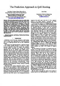
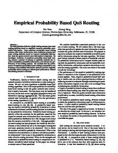
2.1.1 Vehicular Communication Paradigms Communications in vehicular networks fall into three main categories [24] as shown in Figure 2.1. 

Inter-vehicle communication (IVC). This is also known as vehicle-to-vehicle (V2V) communication or pure ad hoc networking. In this paradigm, the vehicles communicate among each other with no infrastructure support. Any

10


valuable information collected from sensors on a vehicle, or communicated to the vehicle, can be sent to neighbouring vehicles. IVC plays a key role in VANETs from two points of view. First, it is necessary to extend the effective range of networked vehicles [25]. Secondly, it might be the only possible communication paradigm especially on highways where a full infrastructure support would incur very high cost to deploy and maintain [26]. 

Vehicle-to-roadside communication (VRC). This is also known as vehicle-toinfrastructure (V2I) communication. In this paradigm, vehicles can use cellular gateways and wireless local area network access points to connect to Internet and facilitate vehicular applications.



Inter-roadside communication. This is also known as hybrid vehicles-toroadside communication. In this paradigm, road infrastructure equipment can communicate among each other and share information about the traffic status. Moreover, vehicles can use road infrastructure to communicate and share information with other vehicles in a peer-to-peer mode through ad hoc communication. The communication between vehicles and the infrastructure can be either in a single hop or multi-hop fashion depending on their position. This paradigm includes V2V communication and provides greater flexibility in content sharing.

Figure 2.1

Vehicular Communication Paradigms [27]

11


Other emerging communication paradigms such as Vehicle-to-Pedestrian (V2P) and Vehicle-to-Motorcycle (V2M) are being developed as new safety technologies by automakers such as Honda motor company [28].

2.1.2 Special Features and Challenges Similar to MANETs, nodes in VANETs self-organise and self-manage the information in a distributed fashion, i.e., without a centralised server controlling the communications [24]. This means nodes can act as servers and/or clients at the same time and exchange information with other nodes. However, nodes in VANETs have special attractive features over MANETs and other wireless sensor networks. These features are [29] 

Unrestricted transmission power and storage. Mobile device power issues are not usually a significant constraint in VANETs since the vehicle can provide continuous power for computing and communication devices.



Higher computational capability. It is assumed that vehicles can provide the communication devices on board with significant computing and sensing capabilities.



Predictable mobility. Unlike MANETs, vehicles’ mobility can be predictable because they move on roadways under certain traffic regulations. Information about these roadways is often available from a positioning system like Global Positioning System (GPS). If the current position and velocity of the vehicle and the road trajectory are known, then its future position can be predicted.



Vehicle registration and periodic inspection. Vehicles have an obligation to register with a governmental authority and be regularly inspected. This feature is unique for VANETs and can offer significant advantages in terms of checking the communication system integrity and security information updates. Besides the pleasing features mentioned above, there are some technical

challenges raised by the unique behaviour and characteristics of VANETs. These challenges should be resolved in order to deploy these networks effectively and bring the proposed applications to fruition. These technical challenges include [29]

12




Potentially large scale. VANETs are almost the only ad hoc network that expected to have hundreds of nodes participating in the communication process. Network nodes include vehicles and potential road infrastructure such as RSUs. Therefore, VANETs should be scalable with a very high number of network nodes.



Partitioned network. Vehicular networks are characterised by a highly dynamic environment and rapidly changing topology. These characteristics could lead to large inter vehicles gaps in sparse scenarios and results in many isolated clusters of vehicles. Pedestrian crossings, traffic lights, and similar traffic network conditions are examples of reasons for frequent network partitions.



Propagation model. The vehicular network environment is not supposed to be a free space. Hence, building, trees, and other vehicles should be considered while developing the propagation model.



Reliable communication and MAC protocols. VANETs experience multi-hop communications that provide a virtual infrastructure among moving vehicles. In fact, this poses a major challenge to the reliability of communication and the efficiency of the Medium Access Control (MAC) protocols that have to be in place.



Routing. Since the network topology is rapidly changing, communication links suffer from fast variation and are vulnerable to disconnection. Consequently, routing algorithms should be efficient and provide a reliable routing service for the developed applications in VANETs.



Security. Security and privacy are primary concerns in VANETs due to the openness of their wireless communication channels to both external and internal security attacks. Appropriate security mechanisms should be in place for providing availability, message integrity, confidentiality, and mutual authentication. On the other hand, real time constraints, data consistency liability, key distribution, and high mobility are examples of the main security challenges, which we describe later.

13


2.1.3 Current Trends and Promising Applications Government agencies, automakers, research institutes, and standardisation bodies are collaborating on various aspects to realise VANETs in our roads. In the US, The Federal Communications Commission (FCC) has allocated 75 MHz of licensed spectrum in the 5.9 GHz as the Dedicated Short Range Communication (DSRC) band for ITS [30, 31]. DSRC is a wireless technology designed to support a variety of applications based on vehicular communications. It utilises the IEEE 802.11p wireless access for vehicular environment (WAVE) standard for the physical layer and the MAC sublayer [32, 33]. Besides that, DSRC requires each vehicle to broadcast a routine traffic message called a Basic Safety Message (BSM), also known as a beacon, every 100 ms. Once automakers start adding the VANET technology to all new cars, it will take 15 years or more for half the cars on US roads to be equipped, according to Qualcomm [34]. Besides being built into new cars, the technology could also be retrofitted easily into older cars [35]. Although safety related applications were the main motivation behind the development of VANETs, other vehicular infotainment applications have emerged. Therefore, applications in VANETs can be categorised as follows 

ITS services. This category includes two sub categories: safety applications and traffic management applications. Safety applications monitor the state of other vehicles and assist drivers in handling the upcoming events or potential danger [36]. Reporting accidents, collision warnings, road hazard notification, and activating emergency brake lights are examples of these applications. On the other hand, traffic management applications aim to share traffic information among vehicles, road infrastructure, and centralised traffic control systems. This information would enable more efficient and smarter use of transport networks. Congested road notification, variable speed limits, adaptable traffic lights, and automated traffic intersection control are examples of these applications.



Non-ITS services. This category is also known as commercial applications. It aims to improve the driving experience and provide leisure services to drivers

14


and passengers. Parking payments, Web surfing, and multimedia services are examples of these services.

2.2 Vehicular Traffic Flow Modelling An understanding of vehicular traffic flow characteristics and vehicular mobility models is essential before developing new algorithms for VANETs, specifically routing algorithms. It helps to adapt the design of the routing algorithm to the properties of the vehicular network environment it is proposed for. Furthermore, vehicular traffic flow may offer some advantages that could be utilised by the routing algorithm to provide a reliable routing service. In traffic theory, vehicular traffic flow is the study that aims to mathematically describe the interactions between vehicles and road infrastructure. This description helps to better understanding and developing road networks with more efficient use and less traffic congestion problems. Vehicular traffic flow models become an essential tool for analysing traffic flow and making decisions on traffic management. They also allow simulation experiments to be performed on virtual traffic when it is not feasible to perform experiments using real-life traffic flows.

2.2.1 Classification of Vehicular Traffic Flow Models Since 1955, when kinematic waves were used to describe the traffic flow on long crowded roads [37], the challenge of mathematically describing vehicular traffic flows has received much interest and become an active area of research. Hence, a wide spread of vehicular traffic flow models have been developed describing different aspects and types of vehicular traffic flows. These models have been categorised from different points of view. We discuss traffic models that are classified according to the following points in [38]. 

Scale of independent variables. Traffic flow models describe dynamic systems where the time scale is a logical classification. A continuous traffic flow model describes the state changes of the traffic system continuously over time. In contrast, a discrete traffic model describes the state changes at discrete time instants.

15




Level of detail. Depending on the domain, the traffic flow model is selected in accordance with the level of detail required in order to represent the traffic system. According to the description level of the traffic system’s entities, there are four sub categories o Submicroscopic models. These models provide a highly detailed description of individual traffic system entities like vehicles and drivers and their interactions. In addition, they model the functioning of subunits of the vehicle behaviour like vehicle control behaviour, e.g., changing gears. o Microscopic models. Similarly to submicroscopic models, they describe the dynamics of individual traffic system entities at a high level of detail. They model actions like acceleration, deceleration, and lane change for each driver as a response to the surrounding traffic. Unlike submicroscopic models, they do not model the functioning of specific parts of the vehicle. o Mesoscopic models. These models provide a medium-level of detail describing small groups of traffic entities and their activities and interactions. They do not differentiate nor trace individual vehicles, but specify the behaviour of individual vehicles, for instance in probabilistic terms. o Macroscopic models. These models describe the traffic flow at a high level of aggregation as the physical flow of a continuous fluid without differentiation of its individual entities. For instance, a traffic flow is described in terms of aggregated macroscopic quantities such as traffic density, traffic flow, and velocity as functions of space and time corresponding to differential equations.



Representation of the process. If the traffic flow model involves processes that use random variables to describe the traffic entities behaviour and their interactions, then it is considered a stochastic model. On the other hand, the deterministic traffic flow model defines all traffic entities and their behaviour using exact parameters.

16




Operationalisation. Traffic flow models can be operationalised either as an analytic solution to a set of equations or as a simulation model.



Scale of application. The application scale indicates the area of application of the traffic model. Some traffic flow models are intended to describe the traffic entities on a highway while others are dedicated to city scenarios and so on.

2.2.2 Vehicular Mobility Models Vehicular mobility models are a key element in realising the study of vehicular networks and their applications. VANETs are almost the only networks that have hundreds or even thousands of mobile nodes that move at high velocities on a constrained topology. The constraints address the interaction among vehicles, road topology, and traffic laws. This feature makes the study of VANETs in a real test bed environment improbable due to logistic difficulties, economic issues, and technology limitations [39]. However, moving to the simulation domain to study vehicular networks requires a certain level of complexity to represent vehicular mobility patterns at an acceptable level of approximation to reality. It is a vital step to develop an appropriate vehicular mobility model before moving on to the simulation phase in order to get adequate results. In the following, we briefly review the state of the art of vehicular mobility models. For a more detailed discussion, we refer the reader to [39, 40]. By definition, vehicular mobility models aim to generate realistic vehicular movement patterns. The traffic flow theory is usually employed to reproduce more real-life like vehicular movements. Mobility models range from the trivial to the realistic. There is always a trade-off between the complexity and the precision of the mobility model. A traditional classification of vehicular mobility models suggests three categories of models are suitable for modelling real traffic flows [39]: macroscopic, mesoscopic, and microscopic. These have been set out above. However, when the mobility model is intended to be used in a network simulation, a different classification has been proposed. It should be noted that network simulators require a high level of detail in order to produce sufficiently accurate results for vehicular networks. Harri et al. [40] propose four distinct classes for the

17


development of vehicular mobility models for simulation purposes, and we discuss them in the following. 2.2.2.1 Synthetic Models In this class, all mobility models are designed based on mathematical models. First, the vehicular movement pattern is grasped and then, a mathematical model is designed to reproduce that movement pattern. The generated movement patters is then validated against real mobility traces gathered from the real world. The main limitation of synthetic models is the complexity of detailed modelling of driver behaviour. Since realistic mobility modelling requires considering behavioural theory, synthetic models can be too complex or impractical at this point. Synthetic models might be separated into five different classes 

Stochastic models. The movement of each vehicle is described at the microscopic level and travel at randomly selected velocities following random paths on the road topology. Stochastic models are the most basic way to describe vehicular mobility.



Traffic stream models. Vehicular mobility is pictured as a continuous flow from a high level. These models determine vehicles’ velocities by leveraging fundamental hydrodynamic physics relationships between the velocity, density, and outflow of fluid. Therefore, they fall into the macroscopic or mesoscopic categories [39].



Car-following models. In this class, the behaviour of each driver is taken into account based on their interactions with neighbouring vehicles using information on position, velocity, and acceleration. These models are categorised as microscopic models.



Queue models. In this class, road traffic is modelled as comprising First In First Out (FIFO) queues and vehicles are modelled as clients.



Behavioural models. Behavioural rules such as social influences determine the movement of each vehicle.

18


2.2.2.2 Survey-based Models Statistics and surveys are an important source of information on mobility patterns and human behaviour. Such surveys on humans’ behaviour, travelling distance, preferred places, etc. can be used by the mobility model to reproduce realistic mobility patterns for a specific region. The UDel mobility model [41] is an example within this category. UDel can model arrival time at work, break and lunch times, vehicular traffic on a workday, and road usage. Survey-based mobility models provide mobility patterns at a macroscopic level. Therefore, they provide more detailed and realistic mobility patterns but still require a complex mathematical model that is calibrated by the survey information. 2.2.2.3 Trace-based Models These models use mobility traces extracted from generic vehicular traffic systems to reproduce more realistic movement patterns. By doing so, significant time can be saved compared to developing a complex mathematical model and calibrating it using survey information. However, this approach has some limitations in terms of the limited availability of vehicular traces and the challenges posed by the need to estimate movement patterns that are not observed directly by the mobility traces. 2.2.2.4 Traffic Simulator-based Models Decades ago, realistic traffic simulators were developed for urban traffic engineering after refining the synthetic models and performing extensive validation using real mobility traces and behaviour surveys. These traffic simulators can model urban vehicular traffic at a very high level of detail at both macroscopic and microscopic levels. They even model energy consumption and pollution, and can be used for noise level monitoring. Examples of such simulators are Corridor Simulation (CORSIM) [42] and Visual Simulation (VISSIM) [43], which are commercial, and Simulation of Urban Mobility (SUMO) [44] and SHIFT [45], which are free. Traffic simulators require configuring a large set of parameters. In addition, the output of traffic simulators cannot be used directly by the network simulator since they have not been designed to generate movement traces, e.g., CORSIM does not output anything other than statistics that copyrights forbid to change, which is a significant

19


limitation [40]. A middle layer is required between the traffic simulator and the network simulator to parse the traffic simulator output files and feed them to the network simulator. Traffic and Network Simulation (TraNS) [46] and Veins [47] are examples of simulation frameworks that integrate both traffic and network simulators to produce realistic simulations of vehicular networks.

2.2.3 The Highway Mobility Model In order to generate realistic vehicular movement patterns, the authors in [40] suggest a framework for realistic vehicular mobility modelling. This framework includes building blocks such as accurate and realistic topological maps, obstacles, attraction/repulsion points, vehicles characteristics, trip motion, smooth acceleration and deceleration, human driving patterns, intersection management, and time patterns. It can be noticed that obtaining such kinds of information imply a high degree of complexity, so it is preferable to make simplifying assumptions wherever appropriate when designing the mobility model. In this research, we design a simple yet realistic vehicular mobility model that is tailored to our simulation needs for a highway scenario. Since highway motion patterns are not too complex, we develop a mathematical model that includes a simple behavioural parameter in accordance with the traffic theory rules. After that, we validate our developed model by comparing the generated movement patterns against those generated by the SUMO traffic simulator. In the following, we explain the development process of our highway mobility model in detail. 2.2.3.1 The Design Approach As described earlier, there are two major approaches to describe the spatiotemporal propagation of vehicular traffic flows [48]: macroscopic traffic flow models and microscopic traffic flow models. The macroscopic approach describes the traffic dynamics in terms of aggregated macroscopic quantities such as traffic density ρveh(x, t), traffic flow qm(x, t), and average velocity vm(x, t) as functions of space x and time t corresponding to partial differential equations. These parameters can be related together through their average values using the following relations [15]

20


dm 

1000

veh

 lm

(2.1)

 dm 1  1000    lm  vm vm  veh 

(2.2)

    1 1   qm   vm  1000  m    lm   veh 

(2.3)

m 

where dm is the average distance between vehicles measured in [m], ρveh is the traffic density on the highway section considered measured in [veh/km], lm is the average length of vehicle measured in [m], τm is the average time gap between vehicles measured in [s], vm is the average velocity of vehicles on the road measured in [m/s], and qm is the average traffic flow measured in [veh/s]. On the other hand, the microscopic approach describes the motion of each vehicle individually. Both macroscopic and microscopic approaches can be utilised together to accurately describe individual vehicle motion and general traffic flow status [49]. Hence, the average velocity quantity offered by the macroscopic approach can be utilised to consider the mathematical distribution of vehicular movements over the traffic network. Moreover, the connection availability between two vehicles is determined based on their position, direction, and velocity, so that using a microscopic approach can improve the accuracy of the modelling. We propose using a hybrid approach combining both macroscopic and microscopic traffic flow models. In this way, the vehicular velocity distribution comes from the macroscopic model while each vehicle's movement is tuned using the microscopic model to refine the prediction of its movement. By using this hybrid approach, we can get a more accurate estimation of the communication link status between two vehicles at any time instant. This is due to the accurate information on the current vehicle status obtained based on the microscopic model, and the use of the probability density function of velocity values to estimate the future status of the vehicle based on the macroscopic model.

21


Using the microscopic approach, the movement of each vehicle i is defined by the following parameters: current Cartesian position at time t: xi(t) and yi(t), current velocity vi(t), direction of movement αi(t), and acceleration/deceleration ai(t). The following relations describe the highway mobility model using the City Section Mobility (CSM) model [50, 51]:

vi (t  t )  vi (t )  ai (t )t xb,c 

yb,c 

(2.4)

c



vik t cos  ik k b 1

(2.5)

c



vik t sin  ik k b 1

(2.6)

where Δxb,c and Δyb,c are the travelling distances along the x and y directions during time Δt = (tc − tb); ∂t is the time sampling interval between tb and tc; vik is the velocity of vehicle i at time instant k; and αik is the direction of movement of a vehicle i at time instant k. The acceleration/deceleration values have a uniform distribution, i.e., the values of vi(t + Δt) do not follow a normal distribution. One possible

solution

is

to

convert

the

uniform

distribution

of

the

acceleration/deceleration values to a normal distribution using the Box-Muller transform [52] or the Ziggurat algorithm [53]. However, this solution is computationally expensive to apply and adds complexity to the highway mobility model. We propose a simpler solution to allow vehicles to accelerate or decelerate or keep the same velocity by picking a new normally distributed velocity value. Let Vset = {nv1, nv2…nve} be a set of normally distributed velocity values generated at t + Δt. Let nvL and nvS ∈Vset, where nvL > vi(t) and nvS < vi(t). If the vehicle picks nvL, then it is accelerating; otherwise, it is decelerating by picking nvS. The drivers' behaviour parameter (DBR) is included in our proposed highway mobility model to distinguish between drivers who tend to accelerate over the average velocity and drivers who tend to decelerate. Thus, we rewrite (2.4) as follows

nvL vi (t  t )   nvS

if U1  3DBR / 4  otherwise 

22

(2.7)


where U1 is a random variable generated between 0 and 1. The DBR parameter value is set based on highway studies that suggest that about 75% of aggressive drivers tend to favour acceleration over the mean velocity [54]. According to classical vehicular traffic theory, vehicles are assumed to have Poisson distributed arrival times. Thus, the time gaps τm between vehicles are distributed according to the following probability density function (pdf) [55]

p ( m )  qme qm m

(2.8)

Based on (2.8), the pdf of the vehicles' distance dm can be written as follows [15] dm



 veh d m q qm  pd (d m )  m e vm  veh e 1000 vm 1000

(2.9)

where qm is substituted by use of (2.3), and lm is neglected to keep the mathematics simple. Hence, the distance between vehicles is exponentially distributed with the rate Λ = ρveh/1000, where dm > 0. Nonetheless, the pdf presented in (2.9) replaces the velocity of vehicles with a constant average velocity vm, which is not quite accurate due to the fact that velocities are variable due to acceleration/deceleration while driving. However, this simple representation of the pdf of vehicles' distance is suitable for our highway mobility model and simulation scenario design. 2.2.3.2 The Validation Process As mentioned before, the degree of realism of the vehicular mobility model used for network simulation plays an essential role in getting adequate results. Therefore, we validated our developed highway mobility model described above against SUMO. Simply put, the movement traces generated by our highway mobility model are compared to those generated by SUMO. We proceed with our validation using a simulation scenario consisting of a three-lane 5 km highway with the following velocity restriction for each lane 40 km/h, 60 km/h, and 80 km/h, respectively. The SUMO traffic simulator is configured as follows. Each vehicle has a normal distributed velocity value according to the lane restriction. The maximum acceleration is 2.6 m/s2, the maximum deceleration is 4.5 m/s2, and sigma, the driver

23


imperfection parameter, which is usually set between zero and one, is taken to be 0.5. Our highway mobility model is configured as follows. Each vehicle has a normal distributed velocity value according to the lane restriction. The vehicular velocities in each lane follow the normal distribution. We use the typical values of velocity distributions calculated in Table 2.1 [15] where μ and σ2 denote the average value and the variance of velocity, respectively. There is no explicit definition of acceleration or deceleration values. DBR, the driver behaviour parameter, is set to 0.5. Table 2.1 µ [km/h] 30 50 70 90 110 130 150

Velocity Distributions v [km/h] ≈ 40 65 ≈ 90 ≈ 120 ≈ 145 ≈ 170 195

σ [km/h] 9 15 21 27 33 39 45

The following results are obtained by plotting the x position of the vehicle along the simulation time for each mobility model. Vehicles travel in one direction horizontally along the x-axis, i.e., y value is 0. The simulation terminates after 5 minutes or when the vehicle leaves the highway after travelling 5 km. It can be noticed from the following Figures 2.2, 2.3, and 2.4 that movement traces generated by SUMO, denoted as Sumo X, are stable. The reason is the smooth acceleration of each vehicle until it reaches the maximum velocity allowed by the lane restriction. In SUMO, once vehicles reach near the maximum velocity allowed by the lane restriction, the generated velocity values are then almost identical. It behaves as in a real-life scenario when driver usually keeps his/her velocity almost the same while driving in the same lane. On the other hand, our highway mobility model, denoted as Highway X, aims to generate normally distributed velocity values while depending on DBR parameter to determine whether a vehicle is accelerating or decelerating. Therefore, the velocity values generated do not have the same degree of realism as those in SUMO. Nevertheless, the travelled distances for both cases,

24


i.e., x positions against time, are very similar as shown in the following figures for each lane in this experiment.

Travelled distance [m]

3500 3000 2500 2000 Sumo X

1500

Highway X 1000 500 0 0

30

60

90

120

150

180

210

240

270

Time [s]

Figure 2.2

Travelled distance in lane restricted to 40 km/h

5000 Travelled distance [m]

4500 4000 3500 3000 2500

Sumo X

2000 Highway X

1500 1000 500 0 0

30

60

90

120

150

180

210

240

270

Time [s]

Figure 2.3


25

2. Fundamentals of VANETs 5000 Travelled distance [m]

4500 4000 3500 3000 2500

Sumo X

2000

Highway X

1500 1000 500 0 0

30

60

90

120

150

180

210

Time [s]

Figure 2.4


In conclusion, the developed highway mobility model can be listed under the synthetic models category since it is based on a mathematical model described by traffic theory in terms of velocities and arrival times of vehicles. Besides that, it uses a hybrid approach of macroscopic and microscopic models to increase the forecast accuracy of communication links future status. According to the validation results obtained, the developed highway mobility model has a high degree of realism.

2.3 Routing in Vehicular Ad hoc Networks The routing process is one of the key issues that has to be addressed if the demands of applications intended to operate in VANETs are to be met. The expected large number of vehicles and the high dynamics and frequent changing of vehicles’ density raise real challenges for the routing process. On the other hand, high computational and memory capabilities and the availability of additional information should be utilised while developing new routing algorithms.

2.3.1 Taxonomy of VANET Routing Protocols There are different aspects to classify the current ad hoc routing protocols proposed for VANETs. The type of information their design depends on, applications’

26


demands, and the VANETs’ property they employ are examples of these aspects. Even though the aspects seem to be different, all categories have almost the same set of routing protocols. Here, we describe the main categories of ad hoc routing protocols proposed for VANETs based on the information they use and VANETs’ properties they utilise [56-58, 70]. 2.3.1.1 Basic Solutions Routing protocols belonging to this category do not use any specific information about the traffic environment such as traffic density, velocity limits, etc. They operate using the control messages received from neighbouring vehicles. Two classifications can be found in this category 

Topology-based solutions. In this category, routing protocols depend on the network topology, which consists of vehicles and communication links, to perform the data packet routing. Furthermore, topology-based protocols can be classified as reactive and proactive protocols. Using the proactive approach, also called table-driven, the routing protocol maintains coherent and up-to-date routing table information even if there are no data packets to route. The advantage of this approach is that routes are already available to be used providing packets are delivered with low delay. However, the control messages needed to maintain routing table information on paths that might not be used waste a large amount of available resources unnecessarily. Optimized Link State Routing (OLSR) [59] and Destination-Sequenced Distance Vector (DSDV) [60] are examples of proactive routing protocols extended to VANETs. On the other hand, using the reactive approach, also called on-demand, the route is established only when there is data to send. The advantage of the reactive approach is the available resources are used only when they are needed. However, in a highly dynamic network, the desired route might not be available, so the communication is delayed until a new route is discovered. Ad hoc On-Demand Distance Vector (AODV) [61], Message Delivery Delay (MDD) [62], and Dynamic MANET On-Demand Routing (DYMO) [63] are examples of reactive routing protocols extended to VANETs.

27




Position-based solutions. In this category, routing protocols use information about the physical locations of network nodes in order to route the data packets. The position of the destination node can be obtained via location management service or by flooding in the expected destination area. When the source node has data to send, it includes the location of the destination node in the header of the data packet. Each node that receives this packet makes its routing decision based on its location, obtained via GPS or other positioning service, and the location of the destination found in the header of received data packet. The advantage of this approach is that the control overhead needed is small because nodes do not discover the route explicitly or maintain routing table information. However, the operations of updating/obtaining nodes location still require some extra overhead. Since these protocols rely on the position information, the inaccuracy of this information, when the network dynamic increases, leads to false routing decisions and consequently, degrades the performance significantly. Another disadvantage is that position-based routing protocols should cope with situations such as no node can be found in the current geographic area. GeoSpray [64] and Position-based Routing using Learning Automata (PBLA) [65] are examples of position-based routing protocols.

2.3.1.2 Map-based Solutions In this category, routing protocols depend on a street-level map to set the junctions needed to get to the destination node. After that, geographic routing is applied to route the data packets through each street until they reach their destination. It is assumed that each node is equipped with a pre-loaded digital map that provides traffic statistics on the roads at different times of the day and traffic signal schedules at intersections. The enhanced Message Dissemination based on Roadmaps (eMDR) [66] and GeoSVR [67] are examples of map-based routing protocols. The advantage of this method is that the whole route is pre-computed and included in the header of every data packet sent from the source node. Thus, the control overhead is kept at a minimum level. However, a pre-loaded street-level digital map might not be available at every node.

28


2.3.1.3 Trajectory-based Solutions Since vehicles are equipped with multiple sensors such as odometers and speedometers, the current trajectory of the vehicle can be obtained easily. Routing protocols in this category use trajectory information of neighbouring vehicles to route the data packets to the destination. If the current vehicle finds a neighbour whose trajectory goes closer to the destination than its own, it forwards the data packets to that neighbour. This approach implies using a store-carry-forward scheme while routing the data packets. The routing decision at each node is based on the trajectory information received from neighbouring vehicles. Thus, the accuracy of this information plays an essential role in routing the data packets correctly. In addition, when trajectory information is out-dated, a node carries the data packet until receiving updated information from neighbouring vehicles. Therefore, these routing protocols are more suitable for delay tolerant data. Geographical Opportunistic Routing (GeOpps) [68] and Motion Vector (MoVe) [69] are examples of trajectory-based solutions. 2.3.1.4 Mobility-based Routing Protocols In this category, the mobility information is used by the routing protocol to predict the lifetime of available links while making the routing decisions. Mobility information

includes

relative

distance,

relative

velocity,

relative

acceleration/deceleration, and direction of movement. Therefore, routing decisions can be taken on the basis of the lifetime of a communication link or the direction of mobility. However, this method has extra control messages overhead because vehicles should send mobility status update messages to their neighbours to keep them informed. Prediction-Based Routing (PBR) [54] and Receive on Most Stable Group-Path (ROMSGP) [71] are examples of mobility-based routing protocols. 2.3.1.5 Infrastructure-based Routing Protocols The road infrastructure such as RSUs, cellular base stations, and even routine buses are used in routing protocols belonging to this category. RSUs are considered fixed reliable nodes connected together by high bandwidth, low delay, and low bit error rates links. Therefore, they can be used to relay data packets to the destination.

29


However, the deployment of such infrastructure is costly and limited to specific areas. Differentiated Reliable Routing (DRR) [72] and Bus [73] are examples of infrastructure-based routing protocols. 2.3.1.6 Probability-based Routing Protocols Here, the probability theory is used to build a probability model of the wireless communication link between two vehicles. After that, it is used to describe the likelihood of certain events like the probability of link breakage or the probability that the wireless link will stay connected for a certain time interval. The routing protocol then chooses reliable links to route the data packets based on their probabilities. Reliable and Efficient Alarm Message Routing (REAR) [74], DeReq [16] and GVGrid [75] are examples of probability-based routing protocols.

2.3.2 Multi-Constrained QoS Routing in VANETs As mentioned earlier, different types of data traffic such as background, voice, and video are expected to be transmitted over VANETs. In order to support the transmission of different data traffic flows, the routes established between the communicating vehicles should meet the QoS requirements of each data type. The QoS requirements are defined by a set of service requirements known as QoS constraints that should be met by the network while transmitting a stream of data packets from the source to the destination [76]. QoS constraints can be grouped into additive and min-max concave constraints. Multiplicative constraints, e.g., packet loss rate, are included in additive class, because they can be transformed into additive constraints by using logarithms [77]. For additive QoS constraints, the value, sometimes called the weight, of the constraint along the route is the sum of the weights on the links forming that route. End-to-End delay and hop-counts are examples of additive QoS constraints. For min-max QoS constraints, the value of the constraint is the minimum or maximum weight on the links that form the entire route. Link bandwidth is an example of a min-max QoS constraint. In a multi-hop vehicular network, identifying feasible routes subject to multiple QoS constraints features a Multi-Constrained (Optimal) Path (MC(O)P)

30


selection, which is proven to be an NP-hard problem [6] if the constraints are mutually independent [78]. Definition 1: Multi-Constrained Path (MCP) problem. Let G(V, E) be an undirected graph representing a vehicular communication network where V is the set of vehicles and E is the set of links connecting the vehicles. Let m denotes the number of QoS constraints Li where i = 1, 2, … m. Each link between two vehicles l(C1, C2) ∈ E is associated with m weights corresponding to QoS constraints such that wi(C1, C2) ≥ 0. The MCP problem is to determine if there is a route P from the source sr to the destination de such that all the QoS constraints are met as described in the following equation:

wi (P) £ Li, i =1, 2, ... m

(2.10)

Definition 2: Multi-Constrained Optimal Path (MCOP) problem. If there is more than one route that satisfies the condition in (2.10), then the MCOP problem is to return the one with the minimum weight with respect to a specific QoS constraint, e.g., the smallest hop-count. 2.3.2.1 Current QoS Routing Algorithms Generally, there are two distinct approaches adopted to solve MC(O)P problems, exact QoS routing algorithms and heuristic and approximation routing algorithms. The main reasons to consider exact multi-constrained routing algorithms are as follows [79]. First, NP-complete behaviour seems to occur in specially constructed graphs, and some exact algorithms are equally complex as heuristics in algorithmic structure and running time on topologies that do not induce NP-complete behaviour. Second, by restricting the number k of paths explored during the path computation, the computational complexity can be decreased at the expense of possibly losing exactness. On the other side, heuristic and approximation algorithms try to reach an approximate solution to the optimal one in polynomial time. There is a wide range of available approximation algorithms to solve the MC(O)P problem. Swarm intelligence based and genetic routing algorithm approaches are relatively novel in this field.

31


In the literature, the appropriate algorithm proposed to solve the MC(O)P problem is usually determined by the number, type, and correlation of the QoS constraints of the problem. Routing with two QoS constraints is not an NP-hard problem unless both constraints are additive. For instance, when the constraints are bandwidth and delay, the MC(O)P problem is defined as a Bandwidth Restricted Path (BRP) problem [80]. Metric ordering is one of the main heuristics utilised to solve the BRP problem. Best paths are computed according to the highest priority metric and are then computed according to the second highest priority metric and so on. Widest-Shortest Path (WSP) and Shortest-Widest Path (SWP) are proposed algorithms to solve the BRP problem using metric ordering. In the WSP algorithm, the first metric to be considered is the number of hops. Shortest paths between the source and the destination are computed. If there is a tie, the path with the highest available bandwidth is chosen. In contrast, the SWP algorithm starts by finding paths with the highest available bandwidth then the shortest path among them is selected. When the two QoS constraints are delay and cost, i.e., additive constraints, the MC(O)P problem is defined as a Restricted Shortest Path (RSP) problem. The proposed algorithms for solving the RSP problem start by computing the feasible paths according to the first constraint. From those feasible paths, they choose the optimal path according to the second constraint if such a path exists. Many heuristics have been proposed to solve the RSP problem, e.g., [78, 81, 82]. Finally, Metric Combination (MC) [83, 84], is another approach proposed to solve the MC(O)P problem when the QoS constraints are correlated. MC is used to reduce the complexity of the MC(O)P problem from multiple constraints to a single constraint. A conventional shortest path algorithm can then be used to find the feasible paths. The problem with this approach is that the combination rule for multiple QoS constraints is not direct and in most cases it is complicated. 2.3.2.2 Challenges of Multi-Constrained QoS Routing in VANETs Due to the highly dynamic nature of VANETs and frequently changing topology, resource reservations are not applicable to provide QoS guarantees. Moreover, the proposed exact QoS routing algorithms are not suitable for solving the MC(O)P problem in VANETs for many reasons. In the exact QoS routing algorithms,

32


different strategies are followed to solve the MC(O)P problem, e.g., nonlinear definition of the path length [85], look-ahead feature [86], non-dominated paths [87], Dijkstra-like path search [83], and k shortest path [88]. Unfortunately, these strategies are not suitable for applications in VANETs. For instance, nonlinear definition of the path length is a fundamental block in achieving an exact solution to an MC(O)P problem. Equation (2.11) shows the nonlinear definition of path P that is known as Holder’s q-vector norm [89] 1

 m  w ( P)  q  q  lq ( P )     i  i 1  Li    

(2.11)

where lq(P) is the path length, wi(P) is the weight value of P according to the constraint i where i = 1, 2, … m, and Li is the constraint value. In this way, the multiconstrained problem is transformed to a single constraint problem enabling the use of Dijkstra’s shortest path algorithm [90] to solve it. It can be seen that the nonlinear definition in (2.11) does not allow prioritising one of the defined constraints over the others, an essential feature needed in VANETs, e.g., video data requires a highly reliable route but is tolerant to delays. Besides that, applying Dijkstra’s algorithm using the above nonlinear definition of the path length in multiple dimensions does not guarantee the subsections of the shortest paths are shortest paths [79]. Therefore, the k-shortest path strategy should be applied along with Dijkstra’s algorithm, which adds extra complexity to the routing process. Furthermore, the look-ahead strategy is another fundamental block in conventional multi-constrained QoS solutions. It proposes to compute the shortest path tree rooted at the destination to each node in the network for each of the m link weights separately [79]. This proposal means that Dijkstra’s algorithm should be executed m times. Thus, the computational complexity becomes m times Dijkstra’s algorithm complexity plus m times the nonlinear length computation complexity. This is also not suitable for VANETs because it adds extra time complexity to the routing algorithm that is supposed to establish routes for real time applications. On the other hand, distributed heuristic solutions such as swarm intelligence based algorithms display several features that make them particularly suitable for

33


solving MC(O)P problems in VANETs. They are fully distributed, so there is no single point of failure, the operations to be performed at each node are simple, they are self-organising, thus robust and fault tolerant, and they intrinsically adapt to traffic changes without requiring complex mechanisms [91]. Ant Colony Optimisation (ACO) is one of the most successful swarm intelligence techniques. It has been recognised as an effective technique for producing results for MC(O)P problems that are very close to those of the best performing algorithms [92]. In ACO, a number of artificial ants build solutions to an optimisation problem and exchange information on the quality of their solutions via a communication scheme that is reminiscent of the one adopted by real ants [22]. However, how and in particular to the degree which the ACO technique can improve multi-constrained QoS routing in VANETs is still unresolved.

2.4 Security Challenges of Robust Routing in VANETs In general, routing algorithms were originally developed without security in mind. In VANETs, vehicles perform routing functions and at the same time act as endsystems thus routing control messages are transmitted unprotected over wireless channels. The QoS of the entire network could be degraded by an attack on the routing process and manipulation of the routing control messages. Security mechanisms that protect the routing process are mandatory for successful deployment of VANETs.

2.4.1 General Security Challenges and Requirements of VANETs Since different stakeholders are involved in the VANET environment, applicable security procedures have to be acceptable to drivers, cars manufactures, service providers, and governments. For example, safety critical information must not be modified or forged in the vehicular network by any authorised, i.e., compromised, or unauthorised, i.e., malicious, vehicle. If a malicious message is detected, then the network should be able to identify and track the vehicle that sent it. However, this ability should not be used to compromise drivers’ privacy. Furthermore, the special characteristics of VANETs feature many security challenges that should be considered while designing security solutions for VANETs. In the following, we

34


briefly present the main security challenges and requirements of VANETs. For more details on these issues, we refer the reader to [93-96]. 

Real time constraints. Delay intolerant data such as safety critical information provided by ITS services has strict transmission delay requirements that should be satisfied. Other information such as vehicle position is also delay intolerant because it loses its accuracy if delivered late. Hence, the cryptosystems selected for such services should not introduce unacceptable delays into the network.



High mobility. Although vehicles have high computational capabilities, the execution time of cryptographic algorithms should be reduced to cope with the high mobility of vehicles, i.e., their execution time should not consume so much of the available communication time between two vehicles that the desired communication cannot take place. Using low complexity security algorithms such as Elliptic Curve Cryptosystems (ECC) and NTRU latticebased cryptography is one of the available approaches to achieve this goal.



Large number of nodes. This feature is another challenge for most existing security approaches. For instance, using symmetric cryptography for mutual authentication would result in a key exchange problem of complexity of O(|V|2) where |V| is the number of vehicles, because every pair of nodes requires a unique shared key, instead of O(|V|) if an asymmetric approach is used [97]. Although using a broadcast authentication technique such as Timed Efficient Stream Loss-tolerant Authentication (TESLA) [98] can help to decrease the complexity of O(|V|2), it may not satisfy the delay requirements of delay sensitive data because of the key disclosure procedure delay such techniques introduce, which we describe later.



Key distribution. This is a block for some security mechanisms and in VANETs raises specific challenges. If the car manufacturer installs the keys, coordination and interoperability among different manufacturers are required. A Certification Authority (CA) can be utilised to certify the vehicle’s public key but vehicles from different countries would have to trust all CAs to authenticate each other, which reduces security. Moreover, driver’s privacy

35


might be violated and a vehicle’s identity could be revealed during key establishment. With regard to the security requirements, we outline the major requirements that need to be met to mitigate attacks and protect the vehicular communication network to the greatest degree possible. Every developed security solution should aim to satisfy the largest group of the following security requirements [93, 99, 100] 

Message authentication and integrity. Message’s contents must be protected against any modification while in transit. Besides that, the receiver of the message should be able to identify the sender. It is worth noting that even though the message’s contents might be authentic, it does not mean the sender of the message is authentic, e.g., if the attacker has control over the sender node.



Non-repudiation. Vehicles that send false or malicious messages or cause accidents must be unable to deny the transmission of these messages.



Message confidentiality. Some messages contents should be kept secret from those nodes that are unauthorised to access them. Driver personal details, payment information, etc. are examples of such contents.



Availability. This is one of the foremost requirements, especially for ITS services. Network overloading, non-cooperative behaviour of some nodes, and Denial of Service (DoS) attacks due to channel jamming may cause network unavailability. It is important to note that availability becomes harder to achieve if the communication links among vehicles are single path or less reliable than available alternatives.



Source authentication. This is an essential requirement for ITS services because their data is life-critical and illegitimate vehicles should not be able to inject false information into the network. A proof of identity mechanism such as digital signatures could be utilised to authenticate the source vehicles.



Mutual authentication. Non-ITS services are supposed to support mutual authentication between clients, i.e., vehicles, and the service provider on one hand and among communicating vehicles on the other hand.

36


2.4.2 Security Threats against the Routing Process In general, attacks on the routing process in an ad hoc network aim to increase the adversaries control over communication between some nodes, degrade the QoS provided by the network, and increase the resource consumption of the victim nodes [101]. An adversary’s capacity to mount specific attacks depends on its nature, i.e., the adversary model. The authors in [102] define three adversary models to classify the adversaries’ abilities 

Membership: Internal vs. External. When the attacker takes control over one of the authenticated vehicles in the network, it is known as an internal attacker. On the other hand, the external attacker is deemed to be an intruder by the network thus the diversity of attacks they can mount is relatively limited. External attackers can be detected if proper security mechanisms are applied.



Method: Active vs. Passive. An active attacker can generate, forge, and inject messages into the network while a passive attacker only monitors the wireless channels and the transmitted messages, e.g., through eavesdropping.



Motivation: Malicious vs. Rational. A malicious attacker has no personal gain from the attacks and aims to jeopardise the performance of the network. On the other side, a rational attacker aims for personal benefits and therefore their behaviour can be predicted in terms of the attack target and attack methods. Due to the fact that vehicles’ communications are not usually protected

physically and may be controlled and compromised by attackers, it can be deduced that VANETs can be subject to any of the above-mentioned adversaries. Usually, the attacker is characterised using the three adversary models, e.g., an internal attacker who is acting passively can mount an eavesdropping attack and monitors the messages exchanged over the network for rational purposes. Routing control messages are the main target of adversaries mounting attacks against the routing process by manipulating and forging the information they contain. This information within the routing control message can be classified into

37


mutable and immutable information. Immutable information is set by the source node and not changed during the routing process, e.g., the source and the destination addresses. In contrast, mutable information is changed at each intermediate node to complete the route discovery process. Changes in mutable information can be classified into traceable changes, e.g., addition of a new intermediate node identifier, and untraceable changes, e.g., an increase in the hop-count value. Protecting immutable information is relatively easy by applying the proper security mechanism such as digital signature. However, protecting the mutable and more specifically the untraceable mutable information such as hop-count is much harder for two reasons. First, intermediate nodes have not yet added some of this information, and the number of nodes that will contribute to this information cannot be anticipated. Second, it is impossible to tell the origin of changes or updates to this information simply by looking at its value, e.g., a hop-count. Besides routing control messages, data messages may also be a target of some attacks, e.g., eavesdropping or modification. However, it is the responsibility of higher layers to detect and mitigate such kinds of attacks against data messages. In the following, we list the main attacks that could be launched by adversaries against the routing process by manipulating the routing control messages [101]. 2.4.2.1 Route Disruption In this attack, an existing potential route between two victim nodes cannot be discovered by the routing protocol due to the adversary. Consequently, the QoS provided by the network is reduced. Other non-victim nodes may also suffer because of the lack of specific routes. There are many techniques for mounting route disruption attacks depending on the routing protocol route discovery mechanism. For instance, the attacker could forge routing error messages and inject them into the network to invalidate a valid link. As a result, the victim node cannot communicate with other nodes. Another way to mount a route disruption attack, in case of ondemand routing protocols, is to flood the network with spoofed routing requests. Therefore, when the victim node wants to find a new route, its legitimate routing requests are considered duplicated and are discarded, i.e., the victim node cannot discover any route. In position-based routing protocols, the adversary can fabricate

38


the location information of the destination by spoofing location update messages. As a consequence, the source will not be able to communicate with the destination. 2.4.2.2 Route Diversion In this attack, the attacker allows the routing protocol to discover a route between two nodes but this route is diverted. The attacker diverts the discovered route through a node he has control over. In this way, he can easily eavesdrop or modify data exchanged between the victim nodes. Thus, the objective of this attack is to increase the adversarial control over the communications between victim nodes. However, this attack has many side effects that may lead the attacker to achieve other objectives. For instance, diverting the discovered route could increase its length and thereby increase the end-to-end delay between the communicating nodes. As a result, the QoS provided by the network is degraded. Simply manipulating or dropping or forging routing control messages can mount the route diversion attack. For example, the attacker can increase the hop-count value in the control message to prevent the discovery of a specific route and force the source node to select a diverted route. 2.4.2.3 Creation of Incorrect Routing State This attack aims at falsifying the information about the routing state in the victim nodes so it appears to be correct while, in fact, it is not. For instance, the routing protocol might return a non-existent route based on an incorrect routing state at some nodes. Consequently, data packets routed using that non-existent route will never reach their destination. Besides that, a routing loop could be created because of an incorrect routing state; hence the data packets will be discarded since their hop-count will exceed the threshold value. The objective of this attack is obviously to degrade the QoS provided by the network. Another objective is to increase the resource consumption at the victim nodes by wasting their resources forwarding data packets based on an incorrect routing state. Forging, modifying, and dropping routing control messages are examples of the techniques followed to create incorrect routing states.

39


2.4.2.4 Generation of Extra Routing Control Traffic In flooding-based routing protocols, attackers can exploit the flooding and mount an attack by injecting spoofed routing control packets to increase the resource consumption. Even if the routing protocol is not flooding-based, e.g., a positionbased, the attacker can still inject spoofed or forged location update messages. This will generate an extra control overhead because of the false location information.

2.5 Summary In this chapter, we reviewed the fundamentals of VANETs related to the aim of this research. The distinctive features of VANETs and its communication paradigms are discussed. We showed that VANETs are a promising technology to enable innovative applications that could prevent accidents and improve the driving experience. However, the unique characteristics of VANETs raise specific technical challenges that need to be resolved first. The vehicular traffic flow modelling and vehicular mobility models are briefly discussed. As a result, we developed a highway mobility model that is tailored to our simulations in this research. After that, we discussed the main categories of routing solutions proposed in VANETs and focused on the QoS routing and its challenges because it is a key feature for many VANETs-enabled applications. Finally, we discussed the security requirements and challenges of VANETs in general and tailored our discussion to the threats that are facing the routing process. We showed that different attacks could be mounted against the routing process that could degrade the performance of the entire network. Therefore, these security threats should be mitigated to provide a reliable and robust routing service in VANETs.

40

3. Reliable Routing Algorithm for VANETs

3 Reliable Routing Algorithm for VANETs Reliable routing is one of the most challenging tasks in VANETs. As mentioned earlier, due to the highly dynamic nature of VANETs and the unpredictable behaviour of drivers, a communication link between two vehicles suffers from fast variation and is vulnerable to disconnection. Therefore, routing reliability needs to be given special attention in order to deploy these networks effectively. In this chapter, we develop a link reliability model for VANETs in order to accurately define the route reliability between two vehicles and improve the reliable routing in VANETs. We consider the route reliability as the first QoS constraint in this research. The first part of this chapter explains the approach taken to calculating the route reliability value accurately based on assumptions made from traffic theory. In the second part, we utilise the evolving graph theory to propose a VANET-oriented Evolving Graph (VoEG) model that helps capture the evolving characteristics of the vehicular network topology and determine the reliable routes pre-emptively.

3.1 State of the Art The literature on routing reliability mainly addresses MANETs [50, 103-106]. For VANETs, Taleb et al. [71] propose a scheme that uses the information on vehicle headings to predict a possible link breakage prior to its occurrence. Vehicles are grouped according to their velocity vectors. When a vehicle shifts to a different group and a route involving the vehicle is about to break, the scheme searches for a more stable route that includes other vehicles from the same group. Namboodiri and Gao [54] introduce a prediction-based routing (PBR) protocol for VANETs. It is specifically designed for the mobile gateway scenario and takes advantage of the predictable mobility pattern of vehicles on highways. PBR predicts route lifetimes and pre-emptively creates new routes before the existing routes fail. The link lifetime is predicted based on the range of communication, vehicles’ locations, and corresponding velocities. Since the route is composed of one or more links, the route lifetime is the minimum of all its link lifetimes. PBR allows the

41


processing of multiple routing requests to check all the available routes to the destination. If the source node receives multiple replies, then it uses the route that has the maximum predicted route lifetime. Menouar et al. [107] propose a movement prediction-based routing (MOPR) algorithm. MOPR predicts the future position of vehicles and searches for stable routes. If several potential routes between the source and the destination exist, MOPR chooses the most stable of the routes composed of stable nodes. Stable nodes are those that move in a similar direction and at a similar velocity compared to the source and the destination nodes. An extension for the routing table in each node is made to fulfil the requirements of this algorithm. The distributions of vehicle velocities and the possibility of sudden changes in network topology are not considered when identifying stable nodes. Kim and Lee [108] propose a block-based routing protocol to identify more reliable paths by predicting the existence of candidate relay nodes when the link expiration time passes. If the vehicle cannot identify a candidate relay node, then the data is rerouted to a different block. The proposed reliable routing protocol extends the geographic routing protocol operating in greedy forwarding mode. They assumed that all vehicles and anchor nodes, i.e., RSUs, are equipped with GPS devices and digital maps. Finally, Bernsen and Manivannan [109] present a position-based reliable routing protocol for VANETs called the reliable inter-vehicular routing (RIVER) protocol. RIVER utilises an undirected graph that represents the surrounding street layout where the vertices of the graph are points at which streets curve or intersect and the graph edges represent the street segments between those vertices. RIVER performs real-time traffic monitoring by actively sending probe messages along streets and passively monitoring messages that are transmitted between adjacent intersections. Reliability ratings are assigned to each street edge while performing the real-time traffic monitoring. These reliability ratings are then used to select the most reliable route. Like other position-based routing protocols in VANETs, RIVER requires a pre-loaded digital map to perform its tasks successfully. It can be noted that all of the above work depends on kinematic information from vehicles to anticipate the future status of a route and deliver data packets using

42


the most stable, i.e., reliable, route in terms of its lifetime. Position, velocity, and direction of movement information are not enough to perform a solid prediction and find reliable routes. The current vehicular network conditions such as the vehicular mobility pattern and the traffic flow distribution have to be considered if the routing algorithm is to be able to consistently find a reliable route. Moreover, it is preferable to eliminate the need for digital maps to perform the reliable routing because it adds extra complexity to the process and maps may not be available for every vehicle on the road. Therefore, reliable routing in VANETs has not yet been well established in the literature and requires further investigation. This investigation is the subject of this chapter.

3.2 Challenges of Reliable Routing in VANETs The technological platform needed for developing and deploying a fully connected transportation system is a combination of well-defined technologies, interfaces, and processes that combined ensure safe, stable, and reliable system operations that minimise risk and maximise opportunities [110]. As a matter of fact, the reliability and stability of the data exchange process are cornerstones of any deployable VANET system. Pedestrian crossing traffic lights and other traffic network conditions are expected to cause frequent network partitions in VANETs that make the reliable routing of data harder to perform. Indeed, a major threat to the reliability of an established route between the communicating vehicles is highlighted. In addition, the expected large number of vehicles and the highly dynamic nature of vehicular networks add complexity to the routing process. On the other hand, routing algorithms can benefit from the mobility constraints and the possibility of predicting the vehicles mobility patterns on the roads to make better routing decisions.

3.3 Vehicular Reliability Model As we have hinted earlier, it is a complicated task to develop a reliable routing algorithm for VANETs because it is influenced by many factors such as the vehicular mobility pattern and the vehicular traffic distribution. In order to define the vehicular reliability model precisely, the mobility model and the vehicular traffic characteristics should be determined first. We utilise the highway mobility model we

43


developed in Chapter 2 and consider vehicular velocity as the major factor in determining the expected communication duration between two vehicles. It is worth noting that wireless channel conditions such as congestion and noise errors could have an impact on the expected communication duration [111]. However, this issue is beyond the scope of this research.

3.3.1 Link Reliability Model We define the link reliability as the probability that a direct communication link between two vehicles will stay continuously available over a specified time period. Given a prediction interval Tp for the continuous availability of a specific link l(Ci, Cj) between two vehicles Ci and Cj at t, the link reliability value rt(l) is defined as follows rt(l) = Prob{to continue to be available until t + Tp | available at t} In order to calculate the link reliability rt(l), we utilise the vehicles’ velocity parameters. Based on the assumption that the vehicular velocity has a normal distribution, the calculation of rt(l) can be done as follows, i.e., if the velocities of two adjacent vehicles are changed or unchanged between t and t + Tp, the resulting relative velocity also has a normal distribution. Let g(v) denote the probability density function of the vehicle’s velocity v, and G(v) be the corresponding probability distribution function  1 g (v )  e  2

( v   )2 2 2

1 G(v  V0 )   2

V0

e

(3.1)



( v  )2 2 2

dv,

(3.2)

0

where μ and σ2 denote the mean and the variance of velocity v measured in [m/s], respectively. The distance d between two vehicles, measured in [m], can be written as a function of the relative velocity Δv and communication duration T, d = ΔvT, where Δv = |v2 – v1|. Since v2 and v1 are normally distributed random variables, then

44


Δv is also a normally distributed random variable and we can write Δv = d/T. Let H denote the radio communication range of each vehicle measured in [m]. The range where the communication between any two vehicles remains possible can be determined as 2H, i.e., when the relative distance d between the two vehicles changes from −H to +H. Let f(T) denote the probability density function of the communication duration T. We can calculate f(T) as follows

f (T ) 

where μΔv

4H 1 e  v 2 T 2 =

|μv1

−



(

2H  v )2 T 2 2v

μv2| and σ2Δv

for T  0

=

(3.3)

σ2v1 + σ2v2 denote the mean and the variance of

relative velocity Δv between two vehicles, respectively. We suppose that each vehicle is equipped with a GPS device to identify its location, velocity, and direction information. Tp is defined as the prediction interval for the continuous availability of a specific link l(Ci, Cj). We assume that vehicles do not change their velocities either by accelerating or decelerating during Tp. We also assume there is no separation distance between lanes carrying forward traffic and lanes carrying backward traffic. The width of the road is ignored for simplicity. The following cases are considered to calculate Tp accurately 

Vehicles are moving in the same direction

ì H + Qij ï ï | vi - v j | Tp = í ï H - Qij ïî | v - v | i j 

ü if v j > vi , C j approchesCi from behind ï ï ý if vi > v j , Ci moves forward in front of C j ï ïþ

(3.4)

Vehicles are moving in opposite directions  H  Qij  v v j  i Tp    H  Qij  vi  v j 

    Ci and C j are moveing away from each other    Ci and C j are moving toward each other

45

(3.5)


where Qij is the Euclidean distance between vehicles Ci and Cj, and vi and vj are the velocities of Ci and Cj, respectively. Qij is calculated as follows Qij  ( yi  y j )2  ( xi  x j )2

(3.6)

where we assume that Qij > 0, i.e., two vehicles cannot be at the same coordinates at the same time. We can integrate f(T) in (3.3) from t to t + Tp to obtain the probability that at time t, the link will be available for a duration Tp. Thus, the link reliability value rt(l) at time t is calculated as follows t T p  f (T )dt rt (l )   t  0

 if Tp  0    otherwise 

(3.7)

the integral in (3.7) can be derived using the Gauss error function Erf. It can be obtained as

  2H    t   v      Erf rt (l )  Erf     v 2     

  2H    v       t  T p     v 2      

when T p  0

(3.8)

where Erf is defined as follows [112] Erf ( w) 

2



w

e

t 2

dt

   w  

(3.9)

0

We refer the reader to Appendix A for the complete derivation process of f(T) in (3.3) and the integral (3.8).

3.3.2 Route Reliability Definition In VANETs, multiple potential routes could exist between the source vehicle sr and the destination vehicle de, where each route is composed of a set of links between the

46


source and the destination. Without loss of generality, for any given route, denote the number of its links as Ω: l1= (sr, C1), l2 = (C1, C2)… lΩ = (CΩ, de). For each link lω (ω = 1, 2… Ω), we denote by rt(lω) the value of its link reliability as calculated in (3.7). The route reliability for a route P, denoted by R(P(sr, de)), is defined as follows 

R( P( sr , de ))   rt (l ) where l  P( sr , de ) and 0  R( P( sr , de ))  1

(3.10)

 1

Suppose there are z potential multiple routes from sr to de. If M(sr, de) = {P1, P2…Pz} is the set of all those possible routes, then the most reliable route is chosen at sr based on the following criterion

arg max PM ( sr , d e ) R( P(sr , de ))

(3.11)

In other words, if multiple routes are available, sr chooses the most reliable route that satisfies the reliability constraint determined by the application. It can be said that the route P is reliable if R(P(sr, de)) is greater than or equal to the reliability constraint required by the data traffic type. For instance, if an application transmits video data, then it could set the reliability constraint to 0.6 since it needs more reliable routes than an application that transmits background data. Therefore, the established route P should satisfy the following condition R(P(sr, de)) > 0.6. We can deduce that the same route could be reliable for a specific data traffic flow while it is not reliable for others. Thus, route reliability is a relative concept and depends on the data traffic requirements.

3.4 Reliability-Based Routing Protocol for VANETs (AODV-R) For the purpose of evaluating our developed route reliability definition, we choose to extend the AODV routing protocol to propose our AODV-R routing protocol, where R stands for reliability. AODV is a reactive routing protocol and can be used for both unicast and multicast routing. When a network node needs a connection, it broadcasts a routing request (RREQ) message to the neighbouring vehicles. Every node that receives this RREQ will record the node it heard from and forward the request to other nodes. This procedure of recording the previous hop is called

47


backward learning [23]. If one of the intermediate nodes has a route to the destination, it replies back to the source node with that route. If more than one reply arrives at the source node, then it uses the route with the least number of hops, i.e., the shortest route. If RREQ arrives at the destination node, a routing reply (RREP) message is sent back to the source node using the complete route obtained from the backward learning as illustrated in Figure 3.1.

Figure 3.1

AODV Route Discovery Process [23]

When a link breakage occurs, a routing error message (RERR) is generated to repair the existing route or discover a new one. AODV sends HELLO messages periodically to ensure the link is still active. In order to fulfil the requirements of our proposed AODV-R routing protocol, we extend AODV routing messages RREQ and RREP, and the routing table entries as follows 1) In addition to the conventional fields of RREQ message such as destination address, originator address, etc., we add the following five new fields to its structure as shown in Figure 3.2(a) 

XPos, YPos contain the coordinates of the vehicle that generates or processes this RREQ.



Speed contains the current velocity of the vehicle that generates or processes this RREQ.



Direction contains the movement angle of the vehicle that generates or processes this RREQ.

48




Route_reliability contains the reliability value of the link/route between the sender and receiver of this RREQ.

2) In addition to the conventional fields of RREP message, we add the following one new field to its structure as shown in Figure 3.2(b) 

Route_reliability contains the final value of the whole route reliability between sr and de. The source node uses this value to decide which route should be chosen if multiple routes between sr and de are found.

3) Finally, routing table entries need to include the following information in addition to the conventional fields such as the destination address, next hop address, cost, etc. as shown in Figure 3.2(c) 

rt_reliability contains the value of the route reliability of this route entry. This value is updated every time a route with a higher reliability value is found for the same destination. …

RREQ ID

XPos

YPos

Speed

Direction Route_reliability

a) AODV-R RREQ structure …

Hop count

Destination address

Original address

Life time

Route_reliability

b) AODV-R RREP structure …

Destination address

Next hop

Seq No

Route timer

State

rt_reliability

c) AODV-R routing table entry structure

Figure 3.2

AODV-R Data Structure. (a) AODV-R RREQ structure, (b) AODV-

R RREP structure, and (c) AODV-R routing table entry structure

3.4.1 Route Discovery Process in AODV-R When sr has data to send, it first looks at its routing table. If a valid route to de is found, then it will use it, otherwise a new route discovery process commences. The source node sr broadcasts a new RREQ message to the neighbouring vehicles and adds its location, direction, and velocity information to this request. Once a neighbouring vehicle Ci receives the RREQ, it calculates the link reliability to sr based on (3.7) and creates/updates a direct link l(Ci, sr). Then, the route reliability

49


value is updated by multiplying its received value by the calculated link reliability value and saving the resulting value in the RREQ message according to (3.10). After that, Ci checks if this RREQ has been processed before or not. If it has been, then we already have a reverse route to sr. If the reliability value of this reverse route is less than the reliability value of the discovered one, then we have a new reverse route with a better reliability value. In this case, the RREQ message is processed again, and the routing table entry is updated. Otherwise, it is discarded. This mechanism allows the intermediate/destination nodes to process multiple RREQs and send multiple RREPs to sr. The following chart in Figure 3.3 describes the processing of an incoming RREQ message in AODV-R at the intermediate/destination vehicle. Begin

Calculate link reliability between this node and the node that sends this RREQ

Insert/Update routing entry for the direct link to the sender node

Update the link reliability value saved in RREQ

No

Is this node the destination?

Insert/update reverse route to the source node

No

Have fresh route to the destination?

Yes

Insert/update routing entry based on the greatest route reliability value

Yes

Create and send RREP back to the source with route reliability value

Broadcast RREQ

End

Figure 3.3

Incoming RREQ process algorithm in AODV-R

50


After finishing the process of creating/updating the reverse route, Ci checks if it is the destination vehicle. If yes, then a RREP message is sent back to sr with the final route reliability value. If it is not the destination, then it checks if it has an active route to de. If there is one, it sends a RREP message back to sr, else it broadcasts the RREQ to other vehicles after updating the relative fields such as XPos, YPos, Speed, etc. When sr receives multiple RREPs for the same RREQ, it selects the route based on the maximum reliability value among all received RREPs according to (3.11). In this way, AODV-R chooses the most reliable route from the source to the destination.

3.4.2 Performance Evaluation of AODV-R We have carried out a six-lane traffic simulation scenario of a 5 km highway with two independent driving directions in which vehicles move. The number of vehicles in each lane is 10 vehicles, i.e., 60 vehicles along the entire highway. We use the highway mobility model developed in Chapter 2, which is implemented in OMNet++. The average velocity of vehicles for each lane is 40 km/h, 60 km/h, and 80

km/h,

respectively.

The

velocity

of

vehicles

is

variable

due

to

acceleration/declaration performed by drivers on the road. We choose randomly two vehicles as the observed vehicles, i.e., source/destination pair, for each simulation run. The most reliable route is chosen at the source node if multiple routes to the destination exist. We compare the simulation results of the AODV routing protocol with AODV-R. AODV is a well-known ad hoc routing protocol that is adopted and extended for routing in VANETs. Most of the on-demand routing protocols, which are proposed for VANETs, are based on the principles of AODV that are modified or tweaked for specific scenarios. Therefore, we choose AODV for this performance evaluation to indicate the improvement that AODV-R can achieve over AODV. As a result, this improvement can be used to compare with related works that are based on AODV or similar approach for the same simulation scenario. Figure 3.4 illustrates the simulation scenario.

51

3. Reliable Routing Algorithm for VANETs 40 km/h 60 km/h 80 km/h 80 km/h 60 km/h 40 km/h

Figure 3.4

Six-lane Highway Simulation Scenario

The highway scenario used in this simulation is of a straight stretch of highway, which does not have hard bends or roundabouts or curves. However, when curves are present in the highway, the link reliability estimation will, in general, not be significantly affected since the only new variable will be the left or right velocity component of vehicles movement. Moreover, the left or right velocity component generally does not affect the link lifetime estimation because it is usually small in value in comparison to the forward or backward velocity component and communication range. 3.4.2.1 Simulation Settings The following simulations were performed 

Experiment A - We change the average velocity of the vehicles in the third lane only from 60 to 140 km/h. The UDP packet size is 1024 bytes. The transmission data rate is 10 packets per second.



Experiment B - We change the data packet size from 500 to 3000 bytes. The transmission data rate is 10 packets per second. The average velocity of the vehicles in each lane is 40 km/h, 60 km/h and 80 km/h, respectively.

The simulation parameters are summarised in Table 3.1. Table 3.1

AODV-R Evaluation – Summary of the Simulation Parameters

Simulation Area Mobility Model

1km x 5km Highway

52

3. Reliable Routing Algorithm for VANETs Communication Range MAC Application Transmission rate Source and Destination vehicles Vehicles’ velocities Vehicles’ distances Number of runs Simulation duration Confidence intervals

450m IEEE 802.11p UDP Burst 10 packets/s Randomly chosen for each simulation run Normally distributed Exponentially distributed 20 300 seconds 95%

3.4.2.2 Performance Metrics The following four performance metrics were considered for the simulations 

Average Packet Delivery Ratio (PDR). It represents the average ratio of the number of successfully received data packets at the destination node to the number of data packets sent.



Average End-to-End (E2E) delay. It represents the average time between the sending and receiving the data packets that are successfully received at the destination node.



Transmission Breakages. It represents the average number of transmission breakages that take place during the data transmission. The transmission breakages metric includes the breakages that occur due to route timeout and loss of connection due to the relative movement of two vehicles. This metric shows the efficiency of the routing algorithm in avoiding transmission failures and delivering uninterruptable data transmission.



Routing Requests Overhead. It expresses the ratio of the total number of routing request messages generated to the total number of data messages sent.

53


3.4.3 Simulation Results 3.4.3.1 Experiment A - Effect of Different Velocities Figure 3.5 shows that the proposed routing protocol AODV-R achieves a higher packet delivery ratio than AODV. It is noticed that the average PDR reduces for both routing protocols when the average velocity in the third lane changes from 60 to 140 km/h. This reduction comes from the fact that the network topology becomes more dynamic and unstable when velocity increases. However, the degradation of the PDR of AODV-R is less rapid than that of AODV. Choosing the most reliable available route makes AODV-R well adapted to the highly dynamic vehicular environment. In AODV-R, when sr receives multiple routing replies, it chooses the most reliable route, which helps reduce the possibility of link breakages and the need for another route discovery process. Fewer route discovery processes means more bandwidth can be allocated for data packet transmission. 80

Packet Delivery Ratio

70 60 50 40 30 20

AODV

10

AODV-R

0 60

Figure 3.5

80

100 120 Velocity in the third lane [km/h]

140

AODV-R Evaluation – Experiment A – Packet Delivery Ratio

54


Average E2E Delay [sec]

0.16 0.14 0.12 0.1 0.08 0.06 0.04

AODV

0.02

AODV-R

0 60

Figure 3.6

80


140

AODV-R Evaluation – Experiment A – Average End-to-End Delay

In Figure 3.6, AODV-R shows higher average end-to-end delay values than AODV. The route establishment in AODV-R takes longer than that in AODV because of the processing of multiple routing requests and replies. However, the established route will be the most reliable one and will be used for a longer time. On the other hand, AODV chooses the shortest route to the destination regardless of its reliability. Thus, the route discovery process in AODV takes less time to find a route, but link breakages have a higher probability of occurring. This is linked to Figure 3.5 that shows that AODV has a lower average delivery ratio than AODV-R especially when the velocity in the third lane exceeds 100 km/h. When a transmission breakage occurs, a RERR message is generated for the purpose of repairing the current route or launching a new route discovery process. Figure 3.7 shows that AODV has a higher average number of transmission breakages than AODV-R. The shortest route selection algorithm of AODV is highly prone to link failures when the network topology becomes more dynamic. On the other hand, AODV-R processes all the possible routes to the destination and chooses the most reliable one. For both AODV and AODV-R, the average number of transmission breakages increases when the velocity increases. However, AODV-R responds better than AODV to changes in the network topology and keeps a lower rate of link failures.

55

Avg. Number of Transmissions Breakages

3. Reliable Routing Algorithm for VANETs 550 500 450 400 350 300 250 200 150 AODV

100

AODV-R

50 0 60

Figure 3.7

80


140

AODV-R Evaluation – Experiment A – Transmission Breakages

Routing Requests Overhead %

65 60 55 50 45 40 35 30

AODV

25

AODV-R

20 60

Figure 3.8

80


140

AODV-R Evaluation – Experiment A – Routing Requests Overhead

Figure 3.8 shows the average routing requests overhead for both AODV and AODV-R. The two routing protocols are affected by the changes in the network topology. In AODV-R, the routing algorithm uses more routing requests messages to establish the most reliable route, so it is expected to have higher routing requests ratio than AODV. However, the routing requests overhead generated by AODV-R is

56


reasonable and close to that generated by AODV. Figure 3.7 shows the larger the number of transmission breakages in AODV, the greater the number of new route discovery processes that are issued. These extra route discovery processes generate more routing requests overhead. Tables B-I to B-IV in Appendix B show the values of the confidence intervals for each figure in this experiment. 3.4.3.2 Experiment B - Effect of Different Data Packet Sizes In Figure 3.9, AODV-R always achieves a higher PDR than AODV over different data packet sizes. Note that large packets may be fragmented. Any link breakages during the delivery process of a fragment of a data packet can cause the failure of the whole data packet delivery. If the delivery fails, then a new route discovery process is needed to find a new route. More route discovery processes generate more routing control messages, which consume bandwidth from the bandwidth available for data transmission. It is important to use the most reliable route to avoid the possibility of a link breakage during the delivery process of data packet fragments. 80

Packet Delivery Ratio %

70 60 50 40 30 20 AODV

10

AODV-R 0 500

Figure 3.9

1000

1500 2000 Data packet size [bytes]

2500

3000

AODV-R Evaluation – Experiment B – Packet Delivery Ratio

57

3. Reliable Routing Algorithm for VANETs 0.11

Average E2E delay [sec]

0.1 0.09 0.08 0.07 0.06 0.05 0.04

AODV

0.03

AODV-R

0.02 500

Figure 3.10

1000


2500

3000

AODV-R Evaluation – Experiment B – Average End-to-End Delay

In this experiment, Figure 3.10 shows that AODV-R also gives higher average end-to-end delay than AODV. The reason is that AODV selects the shortest route hence the route discovery process takes less time than that in AODV-R, which has to process all available routes to select the most reliable one. This is linked to Figure


3.9, which shows that AODV has a lower PDR than AODV-R. 550 500 450 400 350 300 250 200 150 AODV

100

AODV-R

50 0 500

Figure 3.11

1000


2500

3000

AODV-R Evaluation – Experiment B – Transmission Breakages

58

3. Reliable Routing Algorithm for VANETs 65


60 55 50 45 40 35 30

AODV

25

AODV-R

20 500

Figure 3.12

1000


2500

3000

AODV-R Evaluation – Experiment B – Routing Requests Overhead

In Figure 3.11, the average number of transmission breakages in AODV is confirmed to be higher than that in AODV-R. This observation is illustrated in Figure 3.9, where the PDR of AODV-R is shown to be higher than that of AODV. The simple route selection algorithm in AODV has a higher probability of link failures even though the network topology is not highly dynamic. AODV-R always searches for the most reliable route and keeps a lower rate of transmission breakages. Finally, in Figure 3.12, the average routing requests overhead of both AODV and AODV-R are close to each other as they were in Figure 3.8. The higher rate of transmission breakages in AODV, illustrated in Figure 3.11, causes more route discovery processes to be launched especially when the data packet size increases. These extra route discovery processes increase the routing requests overhead. On the other hand, AODV-R still uses more routing control messages to establish the most reliable route but maintains acceptable levels of routing requests ratio. The Tables B-V to B-VIII in Appendix B show the values of the confidence intervals for each figure in this experiment.

59


3.5 VANET-oriented Evolving Graph Model It can be noticed, from the previous simulation results of AODV-R, that reliable routing process causes high routing requests overhead and high end-to-end delays. Searching for reliable routes in a highly dynamic network topology like a VANET calls for employing different techniques to alleviate the reliable routing process and reduce its overhead. Graph theory can be utilised to help improving the reliable routing process and understand the topological properties of a VANET, where the vehicles and their communication links can be modelled as vertices and edges in the graph, respectively. Recently, a graph theoretical model called evolving graph [17, 18] was proposed to help capture the dynamic behaviour of dynamic networks when mobility patterns are predictable. This model has showed its promising results in MANETs and delay-tolerant networks [113, 114]. We extend the current evolving graph model to capture the evolving characteristics of the VANET communication graph and consider the route reliability metric. The extended evolving graph model helps to determine the reliable routes pre-emptively without broadcasting the routing requests each time a new route is sought. We redesign the reliable routing protocol, AODV-R, to benefit from the advantages of the extended evolving graph model and find the most reliable route with lower routing control overhead, lower average endto-end delays, and less consumption of network resources.

3.5.1 Motivation Recently, the evolving graph model has been extended to better understand the properties of dynamic networks such as MANETs and VANETs. In [115], Monteiro used the evolving graph model to design and evaluate the least cost routing protocols for MANETs with known connectivity patterns. He first implemented an evolving graph based routing protocol, and then it is used to provide a benchmark when comparing ad hoc routing protocols. Monteiro showed that an evolving graph based routing protocol is well suited for networks with known connectivity patterns, and that the model as a whole may be a powerful tool for the development of routing protocols. Pallis et al. [116] focus on providing a thorough study of the topological characteristics and statistical features of a VANET communication graph.

60


Specifically, answers are provided for some critical questions like: How do VANET graphs evolve over time and space? What is the spatial distribution of these nodes? Which are the critical link duration statistics in a VANET when the vehicles move in urban areas? How robust is a VANET? The obtained results could have a wide range of implications for the development of high performance, reliable, scalable, secure, and privacy-preserving vehicular technologies. As a matter of fact, the current evolving graph theory cannot be applied directly in VANETs since the evolving topological properties of the VANET communication graph are not scheduled in advance. Besides, the current evolving graph model cannot consider the reliability of communication links among nodes. In order to fulfil VANETs’ requirements, we extend the current evolving graph model. The extended version of the evolving graph model, called the VANET-oriented Evolving Graph (VoEG), is evolving based on predicted dynamic patterns of vehicular traffic. These patterns are predicted based on the underlying road network and vehicular information. In addition, the VoEG considers the reliability of communication links among vehicles.

3.5.2 Basis of the Evolving Graph Theoretical Model Evolving graph theory [117] is proposed as a formal abstraction for dynamic networks. The evolving graph is an indexed sequence of λ sub graphs of a given graph, where the sub graph at a given index corresponds to the network connectivity at the time interval indicated by the index number, as shown below in Figure 3.13.

B

F 2

[1-3]

4

A 4

C

1, [3-4]

2

E 3

1

G

D

Figure 3.13

1, 4

1, 3

Basic Evolving Graph Model [115]

61


It can be observed from Figure 3.13 that edges are labelled with corresponding presence time intervals. Note that {A, D, C} is not valid journey since edge {D, C} exists only in the past with respect to edge {A, D}. Thus, the journey in the evolving graph is along the route in the underlying graph where its edges time labels are in increasing order. In Figure 3.13, it is easy to find that {A, B, E, G} and {D, C, E, G} are valid journeys while {D, C, E, G, F} is not. Let G(V, E) be a given graph and an ordered sequence of its sub graphs, SG = G1(V1, E1), G2(V2, E2) … Gλ(Vλ, Eλ) such that ⋃𝜆i=1 Gi=G. The evolving graph is defined as Ɠ = (SG, G) where the vertices set of Ɠ is VƓ = ⋃ Vi and the edges set of Ɠ is EƓ = ⋃ Ei. Suppose that the sub graph Gi(Vi, Ei) at a given index i is the underlying graph of the network during time interval Ŧ = [ti-1, ti] where t0 < t1 < ... < tτ, the time domain Ť is now incorporated in the model. Let P be a given route in the evolving graph Ɠ where, P = l1, l2 … lk with li ∈ EƓ in G. Let Pσ = σ1, σ2 … σk with σi ∈ Ť be the time schedule indicating when each edge of the route P is to be traversed. We define a journey J = (P, Pσ) if and only if Pσ is in accordance with P, Ɠ, and Ŧ. This means that J allows the traverse from node Ci to node Cj in Ɠ. Note that journeys cannot go to the past. In the current evolving graph theory, three journey metrics are defined [115]: the foremost, shortest, and fastest journey. They are introduced to find the earliest arrival date, the minimum number of hops and the minimum delay, i.e., time span, route, respectively. Let J = (P, Pσ) be a given journey in Ɠ where P = l1, l2 … lk and Pσ = σ1, σ2 … σk then 

The hop count h(J) or the length of J is defined as h(J)= |P| = k.



The arrival date of the journey a(J) is defined as the scheduled time for the traversal of the last edge in J, plus its traversal time, i.e., a(J) = σk + ƭ(lk).



The journey time t(J) is defined as the time passed between the departure and the arrival, i.e., t(J) = a(J) - σ1.

3.5.3 VANET-oriented Evolving Graph (VoEG) The VoEG model aims to address the evolving properties of the VANET communication graph and consider the reliability of communications links among

62


vehicles. Figure 3.14 illustrates an example of the VoEG on a highway at two time instants: t = 0s and t = 5s.

B (0, 0.42)

A

F (0, 0.28) (0, 0.54)

(0, 0.52)

E

C

(0, 0.32)

(0, 0.2)

(0, 0.81)

(0, 0.46)

(0, 0.9)

(0, 0.44)

G

D

(a) B (5, 0.48)

A

F (5, 0) (5, 0.76)

(5, 0.6)

(5, 0.39)

(5, 0.42)

C

(5, 0)

E (5, 0.8) (5, 0.82)

(5, 0.74)

G

D

(b) Figure 3.14

The proposed VANET-Oriented Evolving Graph (VoEG) Model: (a) at t = 0s; (b) at t = 5s

Each node in Figure 3.14 represents a vehicle on the highway and its corresponding identifier. Different from the corresponding presence time intervals for each edge, i.e., link, used in the conventional evolving graph, we associate the following 2-tuple (t, rt(l)) with each edge, where t denotes the current time and rt(l) denotes the link reliability value at this time t as defined in (3.7). In the VoEG model, the communication link between two vehicles is not available if its reliability value rt(l) equals zero. Unlike the conventional evolving graph, the presence time of the link in the VoEG model is continuous and depends on the current vehicular traffic status. In this case, there is no need to check the order of the presence times of

63


the link when searching for a valid journey. Let l={A, B} be a link in the VoEG where VVoEG is the set of vertices and EVoEG is the set of links. Let Trav(l) be a function that determines whether this link l can be traversed or not

True Trav(l )   False

if 0  rt (l )  1  rt (l )  0 

(3.12)

Figure 3.14(a) shows the VoEG status and the corresponding reliability values associated to each link at t = 0s. All links are eligible to be traversed because

l  EVoEG ,Trav(l )  True . However, if l is eligible to be traversed, it does not necessarily mean that it will be chosen to be part of the optimal, i.e., most reliable, journey. Figure 3.14(b) shows the VoEG status at t = 5s where the associated links’ reliability values change due to the evolving of the VoEG. It can be noticed that links {B, E} and {F, G} are now not eligible to be traversed, i.e., Trav({B, E}) = Trav({F, G}) = False at t = 5s where r5({B, E}) = r5({F, G}) = 0. Furthermore, we introduce a new metric called the journey reliability to our VoEG model to address specifically the routing dynamics of VANETs. Our objective is to find the most reliable journey (MRJ) instead of using the conventional approaches of finding the foremost, shortest, and fastest journey. The MRJ has the highest journey reliability value among all possible journeys from the source sr to the destination de. The new journey reliability metric is defined on the basis of (3.10). Let Ω be the number of links that constitutes a valid journey J between sr and de in Ɠ and rt(lω) be the reliability value of the link lω at time t where J = (P, Pσ) and ω = 1, 2 … Ω. The journey reliability, denoted by R(J(sr, de)), is defined as follows 

R( J ( sr , d e ))   rt (l ) where l  J ( sr , d e ) and 0  R( J ( sr , d e ))  1

(3.13)

 1

i.e., the journey reliability value equals to the product of reliability values of all its formed links. Suppose that there are zj potential multiple journeys from sr to de. If MJ(sr, de) = {J1, J2 … Jzj} is a set of all those possible journeys, then the journey J is chosen based on the following criterion at sr

arg max J MJ ( sr , d e ) R( J (sr , de ))

(3.14)

64


i.e., sr selects the most reliable journey among the possible journeys to de.

3.5.4 Constructing and Maintaining the VoEG Model In VANETs, it is relatively easy to build and maintain the VoEG model at each vehicle in the network because of the availability of additional information on the current vehicular network status. We recall that each vehicle is required to broadcast periodic routine traffic messages, i.e., BSMs, in accordance with the requirement of safety applications and the DSRC standard. These BSMs contain information on the vehicle’s current status such as its location, velocity, direction, etc. Each vehicle that receives a BSM uses its information to construct its VoEG model and define its links. Each link between two vehicles in the constructed VoEG model is assigned with rt(l), the link reliability value. When the vehicle receives routing control messages, it uses the received information to tune and update the information associated with each link. It is worth noting that the VoEG model within each vehicle represents the local vehicular network topology that surrounds it. This is due to the fact that BSMs cannot traverse the whole network topology as they are dropped after a specific number of hops, e.g., 30 hops. In regard to the maintenance process, each vehicle can keep an accurate state of the current VoEG model using the information within the received BSMs and routing control messages and the predicted dynamic patterns of vehicular traffic. The reason that VoEG maintenance process still needs to use the information of the predicted mobility patterns of its nodes, i.e., vehicles, is that the successful reception probability of BSMs is lower than the necessary threshold [118]. Therefore, the successfully received BSMs can be used to tune the current VoEG status. It is important to note that within a specific threshold, the received information at time t on location, velocity, direction, etc. of neighbouring vehicles should be consistent between BSMs and the predicted mobility patterns.

3.6 Evolving Graph-based Reliable Routing Protocol for VANETs After proposing the VoEG model, we redesign the AODV-R routing protocol to

65


benefit from the VoEG advantages and properties. The new design utilises the VoEG model and considers the routing reliability constraint while searching for a route from sr to de. A new routing algorithm to find the MRJ is needed first. Then, this algorithm is utilised to design the route discovery process of our proposed Evolving Graph-based Reliable AODV (EG-RAODV) routing protocol. In order to predict the location of vehicles at a time t, we utilise the highway mobility model we developed in Chapter 2, but with the assumption that vehicles move at a constant velocity v0 along the same direction α0 on the highway. This assumption is reasonable in constrained topologies with similar traffic flows such as highway topologies [50]. We modify (2.5) and (2.6) to meet this assumption as following

xb,c  v0t cos  0

(3.15)

yb,c  v0t sin  0

(3.16)

where Δxb,c and Δyb,c are the travelling distances along x and y directions during Δt = (tc – tb).

3.6.1 The Evolving Graph Dijkstra’s Algorithm (EG-Dijkstra) Finding the most reliable route in the VoEG model is equivalent to finding the most reliable journey, MRJ. For that purpose, we extend the shortest path Dijkstra’s algorithm, since it cannot be applied directly in VoEG, and propose the Evolving Graph Dijkstra’s algorithm (EG-Dijkstra). EG-Dijkstra’s algorithm aims to find the MRJ between sr and de based on the journey reliability definitions in (3.13) and (3.14). The proposed EG-Dijkstra's algorithm maintains an array called the Reliable Graph (RG) that contains all vehicles and their corresponding most reliable journey values. EG-Dijkstra starts by initialising the journey reliability value RG(sr) = 1 for the source vehicle and RG(u) = ϕ for other vehicles. Then for all unvisited vehicles from sr, it finds the journey reliability value based on (3.13) and (3.14). When all neighbours of the current vehicle have been considered, it will be marked as visited

66


and its journey reliability value is marked as final. In the following, pseudo code for the EG-Dijkstra's algorithm is provided. Algorithm 3.1 EG-Dijkstra’s Algorithm Input: A VANET-oriented Evolving Graph VoEG and a source vehicle sr. Output: Array RG that gives the most reliable journeys from sr to all other vehicles. Variables: A set UV of unvisited vehicles. 1. Set journey reliability RG(sr) =1, and RG(u) = ϕ for all other vehicles; 2. Initialise array UV by inserting sr; 3. While UV is not empty do 4. x ←the vehicle with the highest reliability value in UV; 5. Mark x as visited vehicle; 6. For each open neighbour v of x do 7. if Trav(l) is True then 8. Set RG(v) ← rt(l)RG(x); 9. Insert v if not visited in UV; 10. Close x; 11. Return the array RG; Figure 3.15 shows a simple example of EG-Dijkstra’s algorithm with a simple VoEG model at two different time instances: t = 0s and t = 5s. In this example, the source vehicle sr is node 0 and the destination vehicle de is node 5. For ease of illustration, we do not use the 2-tuple notations on the links. Instead, we put the link reliability value only. Each vehicle holds its ID and its RG(ID) value. ϕ

6

0.54

0.95

0.54

0.95

ϕ

3 ϕ

5

6

ϕ

6

1

2 0.43 4

0.43

ϕ

0.21

0.76

1

0.34

0.34 0

1

(i)

0.43 4

0.21

0.76

1

0.25

3 5

2

0.76 4

0.25

0.13

0.43 1

(iii) (a)

67

0.21 1

2 0.43

0.34

4 0.34 0

0.26 0.76

0.34 0

(ii)

0.99

0.43

0.34 1

0.26

0.43

0.34

0.43 0

0.54

0.99

ϕ

2

0.14

0.95

0.09

0.99

0.99 0.21

3 5

0.09

6

0.54

0.95 ϕ

3 5

0.14

1

(iv)

0.34

3. Reliable Routing Algorithm for VANETs ϕ

6

0.58

0.37

6 0.58

0.37

ϕ

3 5

ϕ

6

5

1

ϕ

2

0.89

0.75 4 0.75

1

2

1

4 0.75

0.33

(i)

3 5

2

0.43 1

4 0.75 0

1

(ii)

(iii)

1

2

0.43 1

0.34 0.89

0.75

0.38

0.38

0.33

0.32 0.98

0.34 0.89

0.75

0.38 0.38

0

0.58

0.98

ϕ 0.89

0.75

0.38

0.38 0

0.43

0.19

0.37

0.32

0.98

0.98 0.43

3 5

0.32

6

0.58

0.37 ϕ

3

ϕ

0.19

4 0.75

0.38

0.38 0

1

(iv)

(b)

Figure 3.15

EG-Dijkstra’s Algorithm Example (a) when t = 0s; (b) t = 5s

At t = 0s, (3.15) and (3.16) determine the current locations of vehicles. Then, the links’ reliability values are calculated based on (3.7). EG-Dijkstra’s algorithm discovers vehicles 1 and 4 and assigns the most reliable journey value depending on (3.13) as shown in Figure 3.15(a(i)). Then, it chooses the greatest reliability value and continues to discover vehicle 5. It assigns 0.09 as the most reliable journey value based on (3.14). Although the vehicle 5 is the destination, the algorithm does not stop at this stage as shown in Figure 3.15(a(ii)) because it has to check all possible journeys. In Figure 3.15(a(iii)), the algorithm continues to discover vehicles 2, 3, and 6 and assigns the most reliable journey value for each vehicle. At the end, it arrives to vehicle 5 again from a different journey but by a more reliable route. Thus, the final reliability value is 0.13 and the most reliable journey from vehicle 0 to vehicle 5 at t = 0s is J(0, 5) = {0, 4, 2, 3, 6, 5}. Similar to above, Figure 3.15(b) illustrates the same process at t = 5s. It can be noticed from Figure 3.15(b(iv)) that the most reliable journey now is changed to be J(0, 5) = {0, 1, 5} and its reliability value is 0.32 instead of 0.13 at t = 0s.

3.6.2 The Computational Complexity of EG-Dijkstra’s algorithm The computational complexity of the EG-Dijkstra’s algorithm is similar to the conventional Dijkstra’s algorithm. Let the number of vertices be |V| and the number

68


of edges be |E|. The while loop at step indexed 3 in Algorithm 3.1 is executed |V| times. In step 4, we extract the vertex with the highest reliability value in UV so each vertex will be added exactly once to UV and deleted only once from UV. This task in step 4 takes O(|V|) in the worst case. However, if UV is implemented as a heap, then the computational complexity to extract the vehicle with the highest reliability value at step 4 will be O(log|V|). The edge relaxation process and updating reliability values in the RG array takes O(|E|+|V|). We assume that EG-Dijkstra’s algorithm is proposed to work in the VANET communication graph on highways, i.e., a sparse graph. Thus, we can conclude that the total computational complexity of EG-Dijkstra’s algorithm is O((|E|+|V|)log|V|). As the computational complexity of EG-Dijkstra’s algorithm is similar to Dijkstra’s algorithm, we can say that EG-Dijkstra’s algorithm is a polynomial-time algorithm solving the most reliable route problem [119]. In the worst case, when more vehicles enter the highway, i.e., the sparseness of the VoEG decreases, the computational complexity will be O(|V|2log|V|). However, it should be noted that the number of vehicles that can enter the highway is controlled by the highway’s capacity. The adjacency lists in the source vehicle, where the VoEG is represented, do not grow quickly. Hence, the computational complexity of algorithm does not increase much. Nonetheless, if more vehicles enter the highway, it is suggested to apply the clustering approach, e.g., [116, 120], to keep the computational complexity reasonable.

3.6.3 Route Discovery Process in EG-RAODV It is assumed that sr has the information of the current status of VoEG. When sr has data to send at time t, it calculates the reliability value for each communication link in the current VoEG. Then, EG-Dijkstra’s algorithm finds the MRJ from sr to de. We assume that de exists within the current VoEG and can be reachable from sr via multi-hop routing. At this stage, sr knows the most reliable valid journey to de. It then creates a RREQ message and assigns the hops of the MRJ found as extensions to this RREQ. Note that the extension field in RREQ is not used in the traditional ad hoc routing protocols and was left for future uses. In EG-RAODV, by utilising the

69


extensions information in the RREQ, intermediate nodes can forward the routing request to the next hop without broadcasting. At each vehicle along the route, when a RREQ is received, the information about from which vehicle it heard is recorded. Then, the RREQ is forwarded to the next hop based on the extension’s information. Intermediate vehicles are not allowed to send a RREP message to sr even if they have a valid route to de. Since the time domain is incorporated in the routing process, and the mobility of nodes is highly dynamic, the reliability values at intermediate vehicles might be out-dated. When a RREQ arrives at de, a RREP is sent back to sr to start data transmission. In the following, pseudo code of the EG-RAODV route discovery process is illustrated. Algorithm 3.2 Route Discovery Process in EG-RAODV Input: A VANET-oriented Evolving Graph VoEG and a source vehicle sr and destination vehicle de. Output: The most reliable journey (MRJ) from sr to de. 1. Get the current status of VoEG using (3.15) and (3.16); 2. Calculate the reliability value for all links in VoEG based on (3.7); 3. MRJ ← EG-Dijkstra(VoEG, sr); 4. While MRJ is not empty do 5. x ←the first node from MRJ; 6. Record x in RREQ header as extension; 7. Remove x from MRJ; 8. Send RREQ from sr to de along the most reliable journey; 9. While RREP is not received do 10. wait; 11. Start sending data; It can be noted that EG-RAODV works on a hybrid reactive and proactive basis. The reactive feature in EG-RAODV means that the route will be sought on demand. On the other hand, it finds a route to de based on the VoEG information before sending any routing request, i.e., proactively. By eliminating the broadcasting of routing requests, EG-RAODV is expected to save significant network resources. Besides that, EG-RAODV does not use HELLO messages technique to check the status of links because the entire VoEG is predicted in advance at sr. In terms of route maintenance, EG-RAODV uses the same mechanism used in AODV routing

70


protocol where RERR messages are issued when a link breakage occurs to start a new route discovery process. In case the RREQ does not find the next hop registered in its extension field, e.g., the next hop vehicle stops or leaves the road suddenly, a RERR message is generated and sent back to sr to update the VoEG model and recalculate the most reliable journey.

3.6.4 Performance Evaluation of EG-RAODV The main objective of this performance evaluation is to identify the impact of the highly dynamic topology on the routing process performance of the EG-RAODV routing protocol. Besides that, we want to check the benefits of using the proposed VoEG model in the highway scenario with different data packet sizes and data rates. The simulation results are compared between the AODV [61], OLSR [59], PBR [54], and EG-RADOV routing protocols. The OLSR routing protocol is considered only in the third experiment. As the source code of the PBR routing protocol is not available to us, we implemented it in OMNet++ based on its route discovery process description. In this evaluation, we assume that vehicles move at a constant velocity along the same direction on the highway and that the sr has full knowledge of the VANET communication graph at any given time. We use the same simulation parameters found in Table 3.1, but with 10 runs for each simulation and no confidence intervals are obtained. 3.6.4.1 Simulation Settings The following simulations were performed 

Experiment A - We change the transmission data rate from 32 kbps to 512 kbps. The data packet size is 1500 bytes. Here, the average velocity of vehicles stays constant in the three lanes 40 km/h, 60 km/h and 80 km/h, respectively.



Experiment B - We change the data packet size from 500 to 3000 bytes. The transmission data rate is 128 kbps. Here, the average velocity of vehicles also stays constant in the three lanes 40 km/h, 60 km/h and 80 km/h, respectively.

71




Experiment C - We change the average velocity of vehicles in the third lane only, from 60 to 120 km/h. The data packet size is 1500 bytes. The transmission data rate is 128 kbps.

3.6.4.2 Performance Metrics In addition to the average packet delivery ratio (PDR), transmission breakages, average end-to-end delay, and routing requests overhead from the previous performance evaluation of AODV-R, the following performance metric is considered in experiment C only 

Route Lifetime. It represents the average lifetime of the discovered route. A longer lifetime means a more stable and more reliable route.

3.6.5 Simulation Results 3.6.5.1 Experiment A - Effect of Different Data Transmission Rates Figure 3.16 shows that our proposed EG-RAODV routing protocol achieves higher packet delivery ratio than both PBR and AODV. It can also be seen that EGRAODV obtains a stable PDR performance while the PDR performance of PBR and AODV degrades when the data transmission rate increases. This advantage comes from the fact that EG-RAODV chooses the most reliable route by utilising the extended evolving graph model. Unlike PBR and AODV, no broadcasting of routing requests is needed in EG-RAODV. This saves network bandwidth resources and contributes to a higher data delivery ratio. Figure 3.17 illustrates that the routing requests overhead ratio of EG-RAODV is much smaller than that of both of PBR and AODV. This due to the fact that EGRAODV proactively finds the most reliable route using the VoEG model and directs RREQs based on the chosen route. On the other hand, AODV and PBR keep broadcasting RREQs until they find the destination. It is noticed that PBR has the highest average routing requests overhead because it has to process multiple RREQs in order to find a route to the destination with a maximum predicted route lifetime.

72



60 50 40 30 20

AODV EG-RAODV

10

PBR 0 32

64

128

256

512

Data transmission rate [kbps]

Figure 3.16

EG-RAODV Evaluation – Experiment A – Packet Delivery Ratio

250 Routing Requests Overhead %

AODV EG-RAODV

200

PBR 150

100

50

0 32

64

128

256

512


Figure 3.17

EG-RAODV Evaluation – Experiment A – Routing Requests Overhead

Figure 3.18 shows that the average number of transmission breakages of the EG-RAODV protocol is lower than both of AODV and PBR. AODV chooses the shortest route regardless of whether it is reliable or not. PBR outperforms AODV in terms of transmission breakages because it predicts the link lifetime and creates a

73


new alternative route before a link breakage. Note that with all the different data transmission rates considered, EG-RAODV performs the best. In particular, the gain becomes higher when the data rate increases because the application generates more

Avg. Number of Transmission Breakages

packets to be sent, and more transmission breakages occur with AODV and PBR. 1400 1200 1000 800 600 AODV 400

EG-RAODV PBR

200 0 32

64

128

256

512


Figure 3.18

EG-RAODV Evaluation – Experiment A – Transmission Breakages

Another important advantage of EG-RAODV is its much lower average endto-end delay performance in comparison to both AODV and PBR as shown in Figure 3.19. The achievement of low delay values by EG-RAODV comes from the proactive principle it uses when a new route is sought. As it holds information about the whole VoEG, EG-RAODV can easily predict the current locations of other vehicles and find the most reliable route without broadcasting control messages. On the other hand, AODV causes the highest delay values among the three schemes because it uses a pure reactive approach to find a new route. PBR gives lower delays than AODV since it checks all possible routes to find a stable one to reduce the number of transmission breakages.

74

3. Reliable Routing Algorithm for VANETs 0.1

Avg. E2E Delay [sec]

0.09 0.08 0.07 0.06 0.05 0.04

AODV

0.03

EG-RAODV

0.02

PBR

0.01 0 32

64

128

256

512


Figure 3.19

EG-RAODV Evaluation – Experiment A – Average End-to-End Delay

3.6.5.2 Experiment B – Effect of Different Data Packet Sizes In Figure 3.20, we can see that EG-RAODV always achieves the highest and the most stable PDR performance over different data packet sizes. Note that large packets may be fragmented. Any link breakage during the delivery process of a fragment of a packet can cause the failure of the whole data packet delivery. If the delivery fails, then a new route discovery process is needed. PBR performs better than AODV again because it searches for all possible routes to the destination and chooses the one with the maximum predicted route lifetime. Once again in Figure 3.21, the routing requests overhead ratio of PBR is higher than that of both AODV and EG-RAODV. With the increase in the size of data packets, the number of fragments increases. More routing requests are generated for the route discovery processes due to higher delivery failures caused by additional fragments having to be resent. This explains why the routing requests overhead increases with AODV and PBR. Fortunately, this issue does not affect EG-RAODV because the most reliable route is discovered using the VoEG information.

75



55 50 45 40 35 30

AODV

25

EG-RAODV PBR

20 500

1000

1500

2000

2500

3000

Data packet size [bytes]

Figure 3.20

EG-RAODV Evaluation – Experiment B – Packet Delivery Ratio


160 140 120 100 80 60 AODV EG-RAODV PBR

40 20 0 500

1000

1500

2000

2500

3000


Figure 3.21

EG-RAODV Evaluation – Experiment B – Routing Requests Overhead

In Figure 3.22, the average number of transmission breakages in AODV is confirmed to be the highest and that explains its lowest PDR in Figure 3.20. EGRAODV obtains the lowest number of transmission breakages because it chooses the most reliable route. PBR is designed to choose a route with maximum predicted

76


route lifetime, so it outperforms AODV. However, the simple link lifetime prediction algorithm in PBR is unable to find the most reliable route and hence it results in more link failures than EG-RAODV.

Avg. Number of Transmission Breakages

600 500 AODV EG-RAODV PBR

400 300 200 100 0 500

1000

1500

2000

2500

3000


Figure 3.22

EG-RAODV Evaluation – Experiment B – Transmission Breakages


0.06 0.05 0.04 0.03 AODV EG-RAODV PBR

0.02 0.01 0 500

1000

1500

2000

2500

3000


Figure 3.23

EG-RAODV Evaluation – Experiment B – Average End-to-End Delay

77


In this experiment, EG-RAODV also achieves lower average end-to-end delay than AODV and PBR as shown in Figure 3.23. The delay performance of EGRAODV is not affected by varying packet size. The slight increase in the delay according to packet size in EG-RAODV is because a larger data packet means more fragments to be delivered over the network. One packet is considered fully delivered only when all its fragments are delivered. 3.6.5.3 Experiment C - Effect of Different Velocities The aim of Experiment C is to investigate the impact of different velocities on the routing performance. In this experiment, we also compare EG-RAODV with OLSR as it is a proactive routing protocol. We consider that HELLO and topology control messages in OLSR correspond to the routing request messages in reactive routing protocols. 70


60 50 40 30 AODV EG-RAODV OLSR PBR

20 10 0 60

70

80

90

100

110

120

Vehicles' velocity in the last lane [km/h]

Figure 3.24

EG-RAODV Evaluation – Experiment C – Packet Delivery Ratio

In Figure 3.24, the average PDR reduces for all routing protocols when the average velocity in the third lane increases from 60 to 80 km/h. This reduction comes from the fact that the network topology becomes more dynamic and unstable when the velocity increases. The decrease in the PDR of AODV and OLSR is much rapider than that of EG-RAODV and PBR. To keep the routing tables updated in OLSR, topology control messages are sent to exchange information about the current

78


vehicular status. It is clear that OLSR is not suitable for highly dynamic networks like VANETs. Again, EG-RAODV performs the best in this experiment. In EGRAODV, choosing the most reliable route helps to reduce the possibility of link failure and keeps the highest PDR among the three schemes.


180 160 140 120 100 80 60

AODV EG-RAODV OLSR PBR

40 20 0 60

70

80

90

100

110

120


Figure 3.25

EG-RAODV Evaluation – Experiment C – Routing Requests Overhead

In Figure 3.25, the routing requests overhead ratio generated by EG-RAODV is almost unaffected by the network topology changes. In EG-RAODV, the VoEG model deals with the changes in the network topology. This process is carried out with no need for routing requests broadcasting. On the other hand, all other routing protocols in this experiment are impacted considerably by the changes in the network topology. In particular, PBR creates the highest routing requests ratio due to the need to process multiple routing requests. As more topology control messages are sent in OLSR when velocity increases, its routing requests ratio increases significantly. In Figure 3.26, EG-RAODV and OLSR show lower end-to-end delay values than AODV and PBR. OLSR is a proactive routing protocol, which helps to achieve low end-to-end delays although its delivery ratio is the worst among all the considered schemes as shown in Figure 3.24. The average end-to-end delay values of

79


EG-RAODV are again the lowest and not affected by changes in the network topology. AODV and PBR result in much higher end-to-end delay values when the velocity increases. 0.06


0.05 0.04 AODV EG-RAODV OLSR PBR

0.03 0.02 0.01 0 60

70

80

90

100

110

120


Figure 3.26

EG-RAODV Evaluation – Experiment C – Average End-to-End Delay

In Figure 3.27, EG-RAODV obtains the lowest average number of transmission breakages among all the considered routing protocols. The number of transmission breakages of AODV and PBR increases when the velocity increases. The shortest route selection algorithm in AODV is highly prone to link failures when the velocity of vehicles increases. The PBR prediction algorithm cannot accurately capture the changes of vehicular velocities and hence, it performs worse than EGRAODV. OLSR is not considered in this figure because no transmission breakages are counted in the OLSR simulation experiment since it depends on HELLO messages to maintain the status of links.

80



600 500 400 AODV EG-RAODV PBR

300 200 100 0 60

70

80

90

100

110

120


Figure 3.27

EG-RAODV Evaluation – Experiment C – Transmission Breakages

50

Avg. Route Lifetime [sec]

45 40 35 30 25 20 AODV EG-RAODV PBR

15 10 5 0 60

70

80

90

100

110

120


Figure 3.28

EG-RAODV Evaluation – Experiment C – Route Lifetime

Finally, in Figure 3.28, we show the average route lifetime obtained by AODV, PBR, and EG-RAODV routing protocols. EG-RAODV has achieved a longer route lifetime than both AODV and PBR because it uses the most reliable route in the network, where AODV has the lowest route lifetime value among the three schemes. This observation explains their corresponding PDR relation illustrated in Figure 3.24.

81


3.7 Summary In this chapter, we start an investigation of routing reliability in VANETs by firstly developing a link reliability model based on the mathematical distribution of vehicular velocities on highways. After that, we utilised the developed link reliability model to accurately define the route reliability between two communicating vehicles. The route reliability definition is integrated into the AODV routing protocol to create our reliable routing protocol AODV-R. Evaluation results reveal that AODV-R has a better delivery ratio compared to the conventional AODV since it chooses the most reliable route among all possible routes to the destination. On the other hand, use of AODV-R resulted in higher routing requests overhead and high average end-to-end delays since it had to process all available routes in the network. To overcome these issues, we extended the evolving graph theory and proposed our VoEG model. A new EG-Dijkstra’s algorithm has been developed to find the most reliable journey in VoEG. We redesigned the AODV-R routing protocol to provide the EG-RAODV routing protocol for reliable routing in VANETs. The performance of EG-RAODV has been compared with the reactive, proactive, and PBR routing protocols using extensive simulations with different transmission data rates, data packet sizes, and vehicular velocities. Simulation results showed that EG-RAODV achieves the highest packet delivery ratio among all the tested routing protocols. Its use results in the lowest routing requests overhead because the broadcasting technique is not needed in the route discovery process. As it chooses the most reliable route to the destination, it achieves the lowest number of transmission breakages, the highest route lifetime, and the lowest average end-to-end delay values.

82

4. Situation-aware Reliable Routing Algorithm for VANETs

4 Situation-aware Reliable Routing Algorithm for VANETs As we have described in Chapter 3, reliable routing is a very challenging task in VANETs. Picking the most reliable route in the network does not guarantee reliable communication. The routing algorithm needs to be aware of the current vehicular network conditions, and be prepared for unpredictable changes in the network topology that can cause the current reliable route failure. Within this chapter, we propose applying the situational awareness model to the reliable routing process in VANETs. Our purpose is to approach more reliable routing service by utilising the situational awareness concept than selecting the most reliable route only. In order to do so, the routing algorithm builds a network of reliable links and routes among the communicating vehicles, prepares for immediate recovery of any link breakage when possible at or near the breakage point, and continues to evaluate the current available routes based on the vehicular networks state. In the following, we describe the situation-aware reliable routing algorithm for VANETs but first we shed some light on state of the art and basis of situational awareness.

4.1 State of the Art Apart from military applications where situational awareness is used in vehicular convoy networks [121], to the best of our knowledge, there are no previous studies on applying the situational awareness concept to the reliable routing process in VANETs. However, several studies have been conducted on multipath routing in MANETs and VANETs to achieve a reliable and uninterrupted data transmission. In the context of multipath routing, many routing algorithms have been proposed [122-127]. The main idea is to switch from a primary route to a backup route in the event of primary route failure. There are two main mechanisms for computing multipath routes: node-disjoint and link-disjoint. In the node-disjoint mechanism, e.g., AODV-Multipath (AODVM) [125], each node is allowed to

83


participate in one route only, i.e., no common nodes are allowed between any two established routes other than the source and the destination nodes. Similarly, in the link-disjoint mechanism, e.g., Ad hoc On-demand Multipath Distance Vector (AOMDV) [124], each link is allowed to participate in only one route, i.e., no common links are allowed between any two established routes. According to [128], routes established using the link-disjoint mechanism are only 15-30% more stable than those established using the node-disjoint mechanism with negligible difference in average hop-count. Lee and Gerla [122] propose an on-demand source routing scheme called Split Multipath Routing (SMR) for MANETs. SMR establishes and utilises multiple routes of maximally disjoint paths between the source and the destination nodes. Data packets are then split into these multiple routes to avoid congestion and use network resources efficiently. When a route disconnection occurs, the source node either initiates a new route discovery to replace this route or waits until all routes are broken before commencing a new route discovery process. It can be noticed that SMR produces high levels of routing control overhead because it starts a new route discovery to replace the whole route when a link breakage occurs. Yi et al. [129] propose a Multipath Optimized Link State Routing (MP-OLSR) for MANETs. MP-OLSR is regarded as a kind of hybrid multipath routing protocol, which combines the proactive and reactive features. It sends out HELLO and topology control messages periodically to detect the network topology, just like OLSR [59]. However, MP-OLSR does not always keep an up-to-date routing table. It only computes multipath routes when data packets need to be sent out, i.e., reactively. A multipath Dijkstra’s algorithm is used to provide node-disjoint or linkdisjoint paths when necessary. The whole route from the source to the destination is saved in the header of the data packets. When an intermediate node receives a data packet, it checks the next hop status in accordance with the source route before forwarding this data packet. If the next hop is one of its neighbours, then it forwards the data packet otherwise, the intermediate node re-computes the route and forwards the packet using the new route. Bejerano et al. [130] propose a new strategy called the restoration topology that builds a set of bridges where each bridge protects a portion of the primary route.

84


This strategy needs proper signalling and more advanced switching mechanisms. When a link failure occurs, the restoration topology enables the network to recover by simply activating the bridge protecting that portion of the route. Unlike disjoint routes mechanism, there is no need to switch the whole route to another one. However, this approach requires efficient approximation algorithms to provision the restoration topologies and primary routes simultaneously. These algorithms have high complexity especially when employed in highly dynamic networks such as VANETs. Besides that, VANETs should be represented using a proper dynamic model such as the VoEG model we have proposed in Chapter 3. The restoration topology strategy is beyond the scope of this research. It can be noticed that re-computing the route at intermediate nodes, as in MPOLSR, when the next hop is not available and changing it within the data packet header is not practical in a highly dynamic network such as a VANET. This method introduces high delays to the data packet forwarding process since the new computed route should be changed in each data packet. Besides, neither node-disjoint nor linkdisjoint mechanisms are suitable for achieving a reliable routing service in VANETs. In both mechanisms, the node or the link is usually eliminated from the search space once it has participated in an established route. However, there is no guarantee that the first established route is the most reliable route and thus, each node and link should be available for participating in other routes. We illustrate this point using the following example in Figure 4.1.

0.41

A

0.78

C

E

0.37

0.98

0.99

F

0.88

Direction

B

Figure 4.1

D

0.65

Realistic Case in VANETs

Figure 4.1 shows a realistic case in a VANET where vehicles A, B, C, D, E and F move in two lanes in the same direction. Link reliability values are calculated

85


according to (3.7) and are shown above each link. Suppose that vehicle A is the source node and vehicle F is the destination node. The possible routes existing between A and F are M(A, F) = {(A, C, E, F), (A, B, D, E, F), (A, B, C, E, F), (A, C, B, D, E, F)}. It can be noticed that the number of both node-disjoint and link-disjoint routes between A and F equals one. According to (3.10), the reliability value of each route that exists is R(P(A, C, E, F)) = 0.316, R(P(A, B, D, E, F)) = 0.554, R(P(A, B, C, E, F)) = 0.279 and R(P(A, C, B, D, E, F)) = 0.085. There is no guarantee that the node-disjoint or the link-disjoint mechanisms will choose the most reliable route, which is P(A, B, D, E, F) in this example. If P(A, C, E, F) is computed first, then no other routes can be computed because neither vehicle E in case of the node-disjoint mechanism nor link (E, F) in case of the link-disjoint mechanism are allowed to participate in another route. In order to overcome the drawbacks mentioned above and continue the investigation of routing reliability we started in Chapter 3, within this chapter, we propose applying the Situational Awareness concept and develop the situation-aware reliable (SAR) routing algorithm for VANETs. Unlike the AODV-R algorithm, which picks only the most reliable route, SAR routing algorithm builds a reliable network of links and routes among the communicating vehicles and allows each node or link to participate in more than one route. Moreover, SAR is an on-demand distance vector routing algorithm thus there is no need to include the computed route in the header of data packets. All possible routes between the source and the destination are listed at the source node in accordance with their reliability value. The most reliable route is called the primary route and put into use. The second most reliable route is called the backup route and is saved ready to replace the current one if it turns out to fail, and no recovery is possible near or at the failure point. Therefore, switching the whole route is avoided as much as possible in SAR to ensure a seamless data packets transmission. A new route discovery process is launched only if all reliable routes and links are broken or not valid. Besides that, SAR routing algorithm allows each node to be aware of how the established reliable routes and links evolve over time to ensure their feasibility to use when needed. Needless to say, in the specific scenario of Figure 4.1, a single point of failure that is node E is presented. The proposed solution is supposed to pick up the

86


following two routes from A to F: P(A, B, D, E, F) as a primary and P(A, C, E, F) as a backup. If node E moves out of range of nodes C or D, then both routes turn out to fail. In fact, the destination node F will be unreachable in this case no matter what routing algorithm is used.

4.2 Basis of the Situational Awareness Model Situational Awareness (SA) is the state of being aware of circumstances that exist around us, especially those that are particularly relevant to us and which we are interested in [19]. It describes the perception of the elements in the environment within a volume of time and space, the comprehension of their meaning and the projection of their status in the near future [20]. In this context, the reliable routing process in VANETs can be considered from a situational awareness perspective. McGuinness and Foy [21] extended the definition of SA by including a fourth component called Resolution. In the language of reliable routing process, it refers to the preparation of alternative reliable routes and links for intermediate use if the current route turns out to fail. For a given operator, SA is defined in terms of the operator’s goals and the decisions it has to make [131]. Figure 4.2 shows a situational awareness model that presents four levels of situation awareness, perception, comprehension, projection, and resolution. 

Perception is regarded as level 1 SA and refers to the perception of important information about the current situation. It is an essential level if incorrect decisions are to be avoided later.



Comprehension is regarded as level 2 SA and refers to the understanding of information perceived in the first level of SA. In addition, it tries to integrate multiple pieces of information and determine their relevance to the goals and decisions needed in the current situation. Thus, comprehension offers an upto-date picture of the current situation by determining the significance of the perceived information.



Projection is regarded as level 3 SA and refers to the ability to forecast the future state of the current situation based on the comprehension of

87


information perceived in the first level of SA. This ability to anticipate future events helps take the correct decisions at the correct time. 

Resolution is regarded as level 4 SA and refers to the possible countermeasures that can be taken to manage the risks associated with decisions made based on the projection level. Task Factors . System design . Complexity . Workload . System Capability

State of the environment/ System

Situation Awareness Perception of Elements in Current Situation

Comprehension of Current Situation

Projection of Future States

Resolution of Perceived State

Level 1

Level 2

Level 3

Level 4

Decision

Performance of Action

Individual Factors . Goals .Expectations . Experience .Training . Knowledge

Figure 4.2

The Situational Awareness Model

4.3 Situational Awareness Model for Reliable Routing in VANETs As mentioned earlier, picking the most reliable route in the network does not guarantee a reliable communication. The routing algorithm needs to manage the risks inherent in making routing decisions due to sudden changes in the vehicular network. The SA concept provides a different approach to the reliable routing process. It considers the reliable routing as a continuous process where the routing algorithm chooses the most reliable route in the network, prepares certain

88


countermeasures to be taken when the current route turns out to fail, and continues to evaluate the current solutions based on the state of the vehicular network. In order to do that, vehicles kinematic information, the mathematical distribution of vehicular movements and velocities, and the current vehicular network conditions need to be perceived, comprehended, and analysed. Based on analysis of the results of this process, routing decisions are made to ensure the most reliable route is used. In the following, we discuss the four levels of the proposed SA model for reliable routing in VANETs as shown in Figure 4.3. Environmental Factors . Traffic conditions . Weather status . Accidents . Traffic lights

State of the Vehicular Networks

Situation Awareness Perception of data: location, velocity, direction …etc.

Comprehension of Vehicle status Information

Projection: predict Future vehicles status & find reliable routes

Resolution: Prepare alternative reliable routes

Level 1

Level 2

Level 3

Level 4

Decision

Performance of Action

Individual Factors . Accuracy of information . Goals and objectives . Expectations . Processing mechanisms

Figure 4.3 

Situational Awareness Model for Reliable Routing in VANETs

Perception. Concerning reliable routing in VANETs, perception refers to knowledge of the vehicular network environment conditions such as vehicles’ locations, directions of movement, vehicles’ velocities, traffic conditions, weather conditions, etc. In addition, drivers’ behaviour with regard to their tendency towards acceleration/deceleration is also an important parameter, which the routing algorithm should be aware of. These parameters provide the information needed to determine the current status of

89


the vehicular network and form the basis for the comprehension, projection, and resolution levels of SA. 

Comprehension. Routing algorithms should understand and analyse the available information to provide an up-to-date picture of the current status of the vehicular network for the subsequent SA levels. For example, the synthesis of information on the location, direction, and velocity of two vehicles determines if the two vehicles are moving toward each other or away from each other.



Projection. With regard to reliable routing in VANETs, projection refers to the ability to forecast the future status of the vehicular network and predict link lifetime and its reliability value based on information synthesised from Level 2 SA. In this respect, projection tries to answer the following questions: How reliable is a link between two vehicles? When will this link fail?



Resolution. This level refers to the actions required to recover a route between any two vehicles in case of a link failure. Based on the forecasts from the projection level, the routing algorithm prepares alternative reliable routes and links in case of current route failure. This task can be accomplished by determining a network of reliable links and multipath routes between the communicating vehicles. The most reliable link/route is used, and alternatives are listed according to their reliability value for use if required. The routing algorithm should stay aware of the status of alternative reliable links to ensure their validity as the network topology is highly dynamic and can change very quickly. The proposed model of Figure 4.3 is specifically designed for VANETs to

make routing decisions more reliable. It helps the reliable routing algorithm to establish reliable routes and keep evaluating the current situation to be prepared for an immediate response when the state of the vehicular network changes. As vehicles do not keep moving all the time, i.e., they could stop at a traffic light or leave the road, unpredictable changes could occur in the network topology. These unforeseen changes should be considered while taking routing decisions to reduce their effects on data transmission. Location, velocity, direction, and acceleration/deceleration

90


information are considered as low-level data when perceived by the vehicle, i.e., routing decisions cannot be made based on this data directly. Analysing and synthesising this information in the context of the vehicular network topology allows the routing algorithm to consider the available options and be aware of how the current established links evolve over time. At this point, the perception and comprehension levels are completed. Since the movements of vehicles can be projected into the near future based on the comprehended information, the routing algorithm can weight its available options in terms of a specific constraint, which in this model is the route reliability. Thus, routing decisions are taken based on cooperation between the first three levels of the proposed SA model. To manage the risks inherent in making routing decisions, alternative reliable routes and links should be available to switch if the current route fails. This can be accomplished by considering reliable multipath routes at each node. The resolution level is designed to help the routing algorithm process any link breakage near or at the node it occurs at. In this way, the routing algorithm aims to reduce the effects of link breakages and not disrupt the current data transmission. As a result, routing reliability in VANETs is significantly improved. This improvement is illustrated through simulation results presented later in this chapter.

4.4 Situation-Aware Reliable (SAR) Routing Algorithm In this section, we develop the SAR routing algorithm that implements the defined SA levels in Figure 4.3 and describe the route discovery and route maintenance processes in detail.

4.4.1 Problem Formulation Let G = (V, E) be an undirected graph that represents a vehicular communication network where V is set of vehicles, and E is the set of links connecting the vehicles. A reliability value rt(l) at time t is calculated according to (3.7) and associated with each link l and it is positive. Let Vi denote the set of all neighbours of a given vehicle i, and Sij(P) the set of successor vehicles of i to j associated with route P(i, j). Given sr the source vehicle and de the destination vehicle, SAR routing algorithm aims to define MR(sr, de) = {P1, P2… Pz}, the set of reliable multipath routes available from

91


sr to de where R(P1) > R(P2) >…> R(Pz). P1 is called the primary route, which is the most reliable one and denoted by Pp. P2, P3… Pz are the backup routes ordered by their reliability values and denoted generically as PB. Since the SAR is a distance vector routing algorithm, the following condition is enforced while computing

Ssr de (P) for any route P ∈ MR(sr, de)

Ssr d e (t )  {Cv | R( P(Cv , de ))  R( P(sr , de ))} where Cv  Ssr d e

(4.1)

Assuming that SAR algorithm converges let Vsr denote the set of all neighbours of the source vehicle sr. Equation (4.1) means that if Cv is a successor of sr in a route to de, then the reliability of the route from Cv to de, R(P(Cv, de)), is strictly larger than the reliability value of the entire route from sr to de in accordance with the route reliability definition in (3.10).

4.4.2 Routing Control Messages & Routing Table in SAR Routing control messages are the main part of the developed SAR routing algorithm. To fulfil the requirements of the SA model proposed in Figure 4.3, the routing control message structure should fit the mechanism of processing multiple routing requests, routing replies, and routing error messages. In the following, the structure of routing control messages is explained in detail. 1. SA Routing Request (SARQ) Message. In addition to the conventional fields of a routing request message such as destination address, originator address, etc., the following fields are added. a. Kinematic information contains the coordinates, current velocity, direction of movement, and acceleration/deceleration value of the vehicle that generates/processes the SARQ. b. Link_reliability contains the value of the link reliability between the sender and the receiver of the SARQ. This value is calculated upon receiving SARQ message and updated by the receiver node. c. lasthopID contains the id of the last vehicle that generates/forwards the SARQ. This field is important to prevent nodes from processing a duplicate SARQ, which is generated/forwarded by the same vehicle.

92


d. nextAdvhopID contains the id of the next hop to sr written in the SARQ. This field is essential to prevent loop creation while setting up the reverse route to sr. If the id of the vehicle receiving the SARQ equals the nextAdvhopID field, then the SARQ is discarded. The structure of the SARQ message is shown in Figure 4.4. Type SARQ_ID Link_reliability Direction Destination Address Originator Address

Figure 4.4

Kinematic Information lasthopID nextAdvhopID Destination Sequence Number Originator Sequence Number

SARQ Message Structure

2. SA Routing Reply (SARP) Message. The SARP message is designed to help set up the forward route to the destination node considering the reliability of the traversed route. In addition to the conventional fields of a routing reply message such as destination address, originator address, etc., the following fields are included. a. sarp_id this field is used to prevent nodes from processing duplicate SARP messages. b. Drelia contains the reliability value of the direct link between the node that receives the SARP and the node that forwards it. This field helps with creating direct forward links with the correct link reliability value while the SARP is travelling back to sr. The intermediate node, which forwards the SARP based on the information found in its routing table, updates the value of the Drelia field. In this way, the need to calculate the link reliability value again is avoided. It is assumed that the links are bidirectional, and the reliability values of the links do not change during the lifetime of the route discovery process. c. UpTorelia contains the reliability value of the travelled route from de up to the current intermediate node receiving the SARP. This field helps the intermediate node to establish a forward route to de with the correct reliability value without additional calculation.

93


The structure of the SARP message is shown in Figure 4.5. Type SARP_ID Cost Lifetime Destination Address

Figure 4.5

Drelia

UpTorelia Originator Address Destination Sequence Number

SARP Message Structure

3. SA Routing Error (SARE) Message. Since each node could have multiple routes to neighbouring nodes, it has to be ensured that routing error messages are processed only once to avoid consuming bandwidth available for data transmission. Therefore, the following field is added to the routing error message in addition to the conventional fields such as the originator address, the list of unreachable destinations, etc. a. sare_id contains the id of the SARE message. This field enables the same SARE message generated for the same broken link to be ignored. Besides routing control messages, routing tables play an essential role in routing data packets and routing control messages to their destinations. To fulfil the requirements of the SAR routing algorithm, routing table entries need to include the following information in addition to the conventional fields such as the destination address, next hop address, cost, etc. 

rt_relia contains the reliability value of the corresponded route entry. This value is updated with a higher reliability value if a more reliable route to the corresponding destination is found.



PBstate indicates the state of the route entry, i.e., a primary route or a backup route. This indicator is updated upon discovering a better route in terms of reliability or if the primary route turns out to fail and the backup route becomes the primary one.

4.4.3 Route Discovery Process in SAR Routing Algorithm The route discovery process in SAR aims to define the set of all possible routes between sr and de MR(sr, de) = {P1(sr, de), P2(sr, de) … Pz(sr, de)}. Besides that, intermediate nodes Cv also build their routes to neighbouring nodes in the same way,

94


i.e., reliable multipath routes to other nodes. To achieve this aim, intermediate nodes are allowed to process duplicate SARQ messages while (4.1) is enforced to prevent loop creation. When sr has data to send and no route to de is found, i.e., Ssr de is empty, it issues a new route discovery process by broadcasting a SARQ message. In the following, we provide pseudo code of the SARQ processing algorithm during the route discovery process in SAR in which the notation of Table 4.1 is used. Table 4.1

Notation Used in the SARQ Processing Algorithm

sr de C[ID] Pp, PB, Pd path_relia direct_link() proc_before() reverse_route() destination() forward_route()

The source vehicle The destination vehicle Intermediate vehicle with ID The primary route, the backup route, and the current discovered route, respectively. The link reliability value Check the routing table for a direct link between two vehicles Check if this SARQ has been processed before Search the routing table to find the most reliable reverse route to sr Check if this node is de Search the routing table to find the most reliable forward route to de

Algorithm 4.1 SARQ Processing Input: SARQ message received at vehicle C[j] from vehicle C[i] Output: An updated SARQ is forwarded, or a new SARP is sent back to sr, or SARQ is discarded Variables: Routing table entries and SARQ fields 1. Read the values of SARQ fields including Kinematic information and link reliability value; 2. if SARQ[nextAdvhopID] equals C[ID] then 3. return; 4. Calculate Tp value based on the current information of both vehicles C[i] and C[j]; 5. path_relia  link reliability value according to (3.7); 6. if direct_link(C[i],C[j]) is NULL then 7. insert a new l(C[i],C[j]) in C[j] routing table; 8. else if not proc_before(SARQ) then 9. update l(C[i],C[j]); 10. R(Pd(C[j], sr))  reverse route reliability value according to (3.10); 11. if proc_before(SARQ) then 12. Pp(C[j], sr)  reverse_route(sr);

95

4. Situation-aware Reliable Routing Algorithm for VANETs 13. if Pp(C[j], sr) is NULL then 14. return; 15. else 16. if destination(C[j]) then 17. if R(Pp(C[j], sr)) > R(Pd(C[j], sr)) then 18. PB(C[j], sr)  Pd(C[j], sr); // insert the discovered route as a backup route 19. Send SARP including PB(C[j], sr) information to sr; 20 else 21. PB(C[j], sr)  Pp(C[j], sr);// assign the existing primary route as a backup route 22. Pp(C[j], sr)  Pd(C[j], sr); // insert the discovered route as a new primary route 23. Send SARP including Pp(C[j], sr) information to sr; 24. else 25. if R(Pp(C[j], sr)) > R(Pd(C[j], sr)) then 26. PB(C[j], sr)  Pd(C[j], sr); // insert the discovered route as a backup route 27. return; 28 else 29. PB(C[j], sr)  Pp(C[j], sr); // assign the existing primary route as a backup route 30. Pp(C[j], sr)  Pd(C[j], sr); // insert the discovered route as a new primary route 31. Update SARQ fields with this information; 32 Forward SARQ; 33. else // SARQ is not processed before 34. Pp(C[j], sr)  reverse_route(sr); 35. if Pp(C[j], sr) is NULL then 36. Pp(C[j], sr)  Pd(C[j], sr); // insert the discovered route as a primary route 37. else 38. if R(Pp(C[j], sr)) > R(Pd(C[j], sr)) then 39. PB(C[j], sr)  Pd(C[j], sr); // insert the discovered route as a backup route 40. else 41. PB(C[j], sr)  Pp(C[j], sr);// assign the existing primary route as a backup route 42. Pp(C[j], sr)  Pd(C[j], sr); // insert the discovered route as a new primary route 43. if destination(C[j]) then 44. Send SARP including Pp(C[j], sr) information to sr; 45. else 46. Update SARQ fields with this information; 47. Forward SARQ;

Upon receipt of the SARQ message by the neighbouring node Cj, it is checked that the current node id is not equal to the nextAdvhopID field found in SARQ to avoid loop creation at step 2. If yes, then the SARQ is discarded. Otherwise, Cj calculates the link reliability value l(Ci, Cj) according to (3.7) at step 5. If no direct link is found at Cj, then it inserts this new link in its routing table otherwise it updates the existed direct link if this SARQ is not processed before at steps 6-9. This process ensures that direct links are up to date among vehicles with each route

96


discovery process. The reliability of the route the SARQ has travelled so far from sr to Cj is calculated at step 10 according to (3.10). After that, there are two different paths the algorithm will follow depending on the answer to the following question: Has the SARQ been processed before or not? If it has been processed before, i.e., a duplicate SARQ, then a check is made for an existing primary reverse route entry Pp(C[j], sr) at step 12. If it is found and Cj is the destination node, then the reliability of the current discovered route Pd(Cj, sr) and the reliability of Pp(C[j], sr) are compared at step 17. If R(Pp(Cj, sr)) > R(Pd(Cj, sr)), then Pd(Cj, sr) is inserted as a backup reverse route PB(Cj, sr) at step 18 and a new SARP message is created and sent back to sr with the information of PB(Cj, sr) at step 19. Otherwise, a switch is made where Pp(Cj, sr) becomes a backup reverse route and Pd(Cj, sr) is inserted as a new primary reverse route Pp(Cj, sr) at steps 2122. After that, a new SARP message is created and sent back to sr with the information of Pp(Cj, sr) at step 23. If Cj is not the destination node and R(Pp(Cj, sr)) > R(Pd(Cj, sr)), then a new backup route PB(Cj, sr) is inserted or the existing one is updated at step 26. At step 27 the route discovery process returns because the current node Cj has two routes to sr, primary and backup ones. We limit the listed routes at each node to two routes only to avoid the complexity of listing every route in the network. If the discovered route is more reliable than the existing one, then a switch is done at steps 29-30. The SARQ fields are then updated with the new information and forwarded at steps 31-32 since the discovered route is more reliable than the existing one. In case the SARQ has not been processed before, then Cj checks its routing table for an existing reverse route at step 34. If it is not found, then the discovered route is inserted as the primary route. Otherwise, a comparison between the existing route and the discovered route in terms of their reliability is made at steps 38-42. After that, SAR checks if the current node Cj is the destination node at step 43. If yes, then a new SARP message is created at step 44 with the information of the primary reverse route Pp(Cj, sr), which is the most reliable available route to sr. Otherwise, Cj updates the fields of the SARQ and forwards the SARQ at steps 46-47. Once the algorithm has finished setting up a reverse route to sr, the next step is to forward and process the corresponding SARP message. At Cj, the received SARP

97


is forwarded along both the primary reverse route Pp(Cj, sr) and the backup reverse route PB(Cj, sr) back to sr. In this way, SAR enables sr and intermediate nodes to create primary and backup forward routes to de. The reliability information within the SARP fields is used to create the forward links and routes with the correct reliability values without calculating them again. When an intermediate node receives a duplicate SARP, i.e., it has been processed before and its sarp_id is found in its processed SARPs list, it discards it. Intermediate nodes also discard a forwarded SARP message if it is received from a node that is in its routing table and the next hop toward the destination, which is found in this SARP message, is given as another node in its routing table. In this case, the SARP is discarded without being registered as processed. This is done to allow the intermediate node to process the same SARP if it is received from a node that is not in its routing table. This case is further illustrated via Figure 4.6 below.

0.41

A

0.78

C

0.88

0.37

0.98

B

0.65

D

0.99

F

SARQ Forwarded SARQ with better reliability SARP

Direction of movement

Figure 4.6

E

Example of the route discovery process in SAR where A is the source

vehicle and F is the destination. The primary route is Pp(A,B,D,E,F), its reliability R(Pp) = 0.554, while the backup route is PB(A,C,E,F), with reliability R(PB) = 0.316 Figure 4.6 shows an example of the route discovery process and routing control message dissemination in SAR where each node represents a vehicle on a highway and each link is associated with its reliability value. Vehicle A starts the route discovery process by broadcasting a SARQ message. After disseminating the SARQ in the network, it can be noticed that vehicle E has two reverse routes to A:

98


PB(E, C, A) where R(PB) = 0.31 and Pp(E, D, B, A) where R(Pp) = 0.56. Therefore, vehicle E forwards the received SARQ from vehicle D because it carries a better route back to vehicle A as shown in Figure 4.6. It is worth noting that route cost is not a metric in SAR routing algorithm, e.g., the primary reverse route Pp(E, D, B, A) cost is 3 hops in comparison to 2 hops for the backup reverse route PB(E, C, A). The only metric considered in the SAR is the route reliability. Let us assume the link l(B, D) turns out to fail while using the current primary route Pp(A, B, D, E, F). Since B has received two SARP messages as shown in Figure 4.6, it immediately recovers this breakage by switching to the link l(B, C) toward the destination F. In this case, the data transmission is not disrupted and the switch is made at the breakage point. However, B should be aware of the status of l(B, C) and ensures it is valid before making this switch. This process is further explained in the next section. With regard to SARP messages dissemination, it can be noted that when vehicle C receives the second SARP from vehicle E, which is not shown in Figure 4.6, C discards this SARP even though it is not a duplicate in terms of sarp_id. The reason C has discarded this SARP message is that vehicle E, which C receives this SARP from, is in the routing table of C as part of the existing primary forward route Pp(C, E, F), which is created during the transmission of the first SARP. However, when C receives the SARP from B, it processes it and inserts a backup forward route PB(C, B, D, E, F). It is worth noting that when a SARP is discarded, its sarp_id is not registered as processed to allow the vehicle C to process the same SARP if it is received from a vehicle that is not in its routing table. In this way, although each link is allowed to participate in more than one route, the SAR tries to decrease the degree of link sharing between the discovered routes. In case a routing control message, either SARQ or SARP, has been lost during the route discovery process, the SAR routing algorithm is still able to discover routes between sr and de since it is a multipath routing algorithm. Moreover, the undiscovered route due to the routing control message lost can be obtained in the next route discovery process. If it is more reliable than the current route, then SAR switches to use it.

99


4.4.4 Route Maintenance Process in SAR Routing Algorithm The second important part of the SAR routing algorithm is the route maintenance process. This process represents the implementation of the resolution level of the SA model shown in Figure 4.3. The route maintenance process tries to resolve a link breakage at the node that sensed the breakage before sending a routing error message to other nodes. Besides that, it allows each node to monitor the status of each link with respect to the current vehicular network situation. When a link breakage occurs, SAR first tries to replace the broken link, which is a primary one, with a backup link/route to the same destination if available and valid to use. Once the switching is done, the data transmission will not be interrupted and no SARE messages are issued. In case of no available backup links/routes to switch to, the route maintenance process sends a SARE message to the precursor node assigned with the broken route. The precursor node invalidates the routing table entry that uses the broken link and tries to switch to an available valid backup route. If no available backup route is found, then a routing error message, SARE, is issued to the next precursor node and so on until sr is reached. Finally, sr checks for a backup route to de to switch to which does not include any of nodes that fail to recover the occurred link breakage. A new route discovery process is issued if no available backup route to the destination node exists. Thus, the SAR route maintenance process tries to process link breakages locally at the node level to avoid launching a new route discovery process. In this way, it saves available bandwidth and provides a reliable uninterrupted data transmission service. In order to allow each vehicle to be aware of the current vehicular network conditions, periodic beacons are utilised. Recall that each vehicle is required to broadcast a routine traffic message, i.e., BSM, also known as a beacon, every 100 ms [32]. In this way, each node that receives these beacons can use the information they contain to re-evaluate the current status of each link in its routing table, i.e., reestimate its reliability value. If one of the current links to de is about to break, e.g., the communicating vehicle starts to change its direction to leave the road, then the node can choose to switch to another more reliable link/route to de if such a link/route exists. Otherwise, it issues a SARE message to the precursor node asking it to switch to another link/route to de. This process continues until the switch is

100


done, or sr is reached to start a new route discovery process if needed. By applying level 4 SA and being aware of the current changes in the vehicular network, disruptions to the current data transmission are avoided as much as possible.

4.4.5 Performance Evaluation of SAR In this section, we report the results of simulating the SAR routing algorithm for the six-lane traffic simulation scenario of a 5 km highway illustrated in Figure 3.4 in Chapter 3. However, the traffic density in each lane is variable according to the simulation experiments. Four routing protocols are compared in the simulations: the AODV routing protocol [61], the AODV-R routing protocol, which picks only the most reliable route according to (3.11), the PBR routing protocol [54], and the SAR routing algorithm. 4.4.5.1 Simulation Settings The following simulations are performed: 

Experiment A - We change the number of vehicles on the highway from 15 to 75 vehicles. The average velocity of vehicles for each lane is 40 km/h, 60 km/h and 80 km/h, respectively. The UDP packet size is 2048 bytes. The transmission data rate is 20 packets per second. Note that data packets could be fragmented.



Experiment B - We change the data packet size from 500 to 3000 bytes. The transmission data rate is 20 packets per second. The number of vehicles on the highway is 30 vehicles. The average velocity of vehicles for each lane is 40 km/h, 60 km/h and 80 km/h, respectively.

The simulation parameters are summarised in Table 4.2. Table 4.2

SAR Evaluation – Summary of the Simulation Parameters

Simulation Area Mobility Model Communication Range MAC Application

1km x 5km Highway 450m IEEE 802.11p UDP Burst

101

4. Situation-aware Reliable Routing Algorithm for VANETs Delay Limit Transmission rate Source and Destination vehicles Vehicles’ velocities Vehicles’ distances Number of runs Simulation duration Confidence intervals

1s 20 packets/s Randomly chosen for each simulation run Normally distributed Exponentially distributed 20 300 seconds 95%

4.4.5.2 Performance Metrics In addition to the average packet delivery ratio (PDR), transmission breakages, and average end-to-end delay, the following two performance metrics are considered for the simulations of this performance evaluation. 

Routing Control Overhead. It expresses the ratio of the total generated routing control messages, which includes routing requests, routing replies, and routing error messages to the total number of data packets sent.



Average Dropped Data Packets. It represents the ratio of the average number of data packets that are dropped at the destination node because they exceed the delay limit to the number of successfully delivered data packets. This metric shows the efficiency of the routing algorithm in establishing routes quickly to avoid introducing extra delays to the data packets transmission.

4.4.6 Simulation Results 4.4.6.1 Experiment A - Effect of network density Figure 4.7 depicts the simulation results for the four routing algorithms examined in this experiment. In this figure, the x-axis depicts the number of vehicles in the network while the y-axis depicts the PDR achieved by each routing algorithm. The following observations can be made from this figure. Searching for reliable routes for data transmission in a vehicular network is shown to be an effective way to achieve higher delivery ratios, as evidenced by the performance of SAR and AODVR in comparison to the AODV and PBR routing algorithms. Generally, in Figure 4.7, higher network density enhances the delivery ratio of each examined routing

102


algorithm because more vehicles imply more potential links, so there are more options to establish routes to the destination. With regard to SAR routing algorithm, higher network density helps building a network of more reliable links and routes among the communicating vehicles. It can be noticed that SAR routing algorithm significantly outperforms the other routing protocols considered in this figure. 90


80 70 60 50 40

AODV AODV-R SAR PBR

30 20 15

Figure 4.7

30 45 60 Network Density - Number of Vehicles

75

SAR Evaluation – Experiment A – Packet Delivery Ratio

Figure 4.8 depicts the routing control overhead generated by each routing algorithm examined in this experiment. Although the SAR generates a high routing control overhead, due to the processing of duplicate SARQ and SARP messages, this figure shows it generates an acceptable rate of routing control overhead in comparison with AODV and AODV-R. Note that in the simulations reported the SAR routing algorithm was limited to registering two links/routes entries to the same destination at each routing table if more than one route was available. This was done to avoid the high complexity of using and maintaining all available links/routes to the same destination in a dense connected vehicular network. In Figure 4.8, it is seen that the routing control overhead generated by all the routing protocols increases when the network density increases because more nodes are available for control messages to traverse. The SAR has the benefit of reasonable routing control overhead because it uses the most reliable route in the network and aims to remedy

103


link breakages at the node level rather than the network level. Moreover, using the situational awareness model, SAR allows each node to be aware of the current vehicular network conditions and how they can affect the current established links and routes. This gives SAR routing algorithm a great advantage because a new route discovery process is launched only if there is no valid backup route left to the destination. As a result, the routing control overhead is reasonable in this figure. 40

Routing Control Overhead %

35 AODV AODV-R PBR SAR

30 25 20 15 10 5 0 15

Figure 4.8


75

SAR Evaluation – Experiment A – Routing Control Overhead

Figure 4.9 clearly shows the advantage of SAR in avoiding transmission breakages over other routing algorithms examined in this experiment. To avoid transmission breakages, the routing algorithm should accomplish two steps. First, choosing the most reliable link to ensure it has the longest possible lifetime. Second, being aware of how the established links/routes evolve over time with respect to the changes in the vehicular network topology and respond immediately to the link breakages by activating the backup links/routes. In this way, the information on both current and backup links/routes is kept up to date during data transmission to avoid using out-dated links. The SAR performs those steps by applying the situational awareness levels while searching for reliable routes from the source to the destination vehicles.

104


4. Situation-aware Reliable Routing Algorithm for VANETs 9000 8000

AODV AODV-R PBR SAR

7000 6000 5000 4000 3000 2000 1000 0 15

30

45

60

75

Network Density - Number of Vehicles

Figure 4.9

SAR Evaluation – Experiment A – Transmission Breakages

0.045


0.04 0.035 0.03 0.025 0.02 0.015

AODV AODV-R PBR SAR

0.01 0.005 0 15

Figure 4.10


75

SAR Evaluation – Experiment A – Average End-to-End Delay

In Figure 4.10, it would be natural to expect that the reliable routing process would result in higher delay values for SAR and AODV-R than for conventional routing protocols such as AODV. However, SAR maintains the smallest end-to-end delay values among the routing algorithms examined. Estimating the link reliability values, processing all available links/routes to the destination, maintaining the current established links/routes, and switching between primary routes and backup

105


routes could cause additional delay in transmission. However, it can be observed from Figure 4.10 that the SAR routing algorithm manages to transmit data packets with lower delay. The application of the situational awareness model proposed in Figure 4.3 results in more stable data transmission and fewer transmission breakages, as shown in Figure 4.9. 9 Avg. Dropped Data Packets %

8 7 6 5 4 3 AODV AODV-R PBR SAR

2 1 0 15

Figure 4.11


75

SAR Evaluation – Experiment A – Dropped Data Packets

Figure 4.11 shows the average dropped data packets ratio for each routing algorithm examined in this experiment. The destination node drops the received data packets if they exceed the delay limit, which is set to one second for this experiment. There are two reasons for data packets to arrive at the destination node late. First, the delay caused by the route discovery process affects the data packets that are waiting in the queue to be transmitted. Second, the delay caused by link breakages since data packets should wait until the routing algorithm switches to a valid backup route or finds a new route to the destination node. As the number of vehicles increases, the average number of dropped data packets increases as well. With regard to routing algorithms that process multiple routing control messages, in the cases of AODV-R, SAR, and PBR, when searching for a suitable route, more vehicles in the network means higher delays in the route discovery process. This can be observed via Figure 4.8 where the routing control overhead increases. With regard to routing algorithms

106


that search for the shortest route, in the case of AODV, more transmission breakages, as shown in Figure 4.9, result in a higher delay in the data packets transmission process. The reason for these higher delays is that when a link breakage occurs the routing algorithm has to start a new route discovery process, and data packets have to wait until a new route becomes available. The SAR manages a stable ratio of average dropped data packets because of the high packet delivery ratio it achieves as shown in Figure 4.7, and the low number of transmission breakages as shown in Figure 4.9 thanks to the application of the situational awareness model in SAR. The preparation of alternative reliable links and routes for an immediate recovery of any link breakage, when possible, during data packets transmission, guarantees a seamless transmission with no need to wait for a new route discovery process. Tables B-IX to B-XIII in Appendix B show the values of the confidence intervals for each figure in this experiment. 4.4.6.2 Experiment B - Effect of different data packet sizes The objective of this experiment is to evaluate the ability of the SAR routing algorithm to handle data packet fragments when the transmitted data packet size is larger than the maximum transmission unit (MTU), normally set to 1500 bytes. Figure 4.12 depicts the simulation results for the four routing algorithms examined. In this figure, the x-axis depicts the data packet size in bytes while the yaxis depicts the packet delivery ratio achieved by each routing protocol. It can be observed that SAR achieves higher and more stable performance over different data packet sizes. In addition, AODV-R achieves better performance than AODV and PBR. These achievements of SAR and AODV-R indicate that routing data packets using the most reliable routes in VANETs becomes more significant in the case of large data packets. It is known that large data packets may be fragmented. Therefore, any link failure during the delivery process of these fragments can cause the failure of the whole data packet delivery.

107



80 70 60 50 40 30

AODV AODV-R SAR PBR

20 10 500


Figure 4.12

1000


2500

3000

SAR Evaluation – Experiment B – Packet Delivery Ratio

2400 2100 1800 1500

AODV AODV-R PBR SAR

1200 900 600 300 0 500

Figure 4.13

1000


2500

3000

SAR Evaluation – Experiment B – Transmission Breakages

Since the network topology in this experiment is stable, and no changes occur in terms of the number of vehicles or the velocity of them, the SAR maintains the least number of transmission breakages in comparison to the other routing protocols examined as shown in Figure 4.13. Applying the situational awareness levels to the routing process in VANETs helps reduce the number of potential transmission breakages significantly because routes are established based on the comprehended

108


information of the vehicular network. Besides that, the information on the established routes is kept up to date as the vehicular network topology changes. In this way, SAR avoids using an out-dated link or route and when a sudden link breakage happens, SAR responds immediately by switching to another route when available. It is confirmed via Figure 4.13 that the reliability-based routing protocols are the most appropriate option to be used in this case. In Figure 4.14, the SAR routing algorithm is seen to maintain an acceptable level of routing control overhead in comparison to the other routing protocols examined.


16 14 12 10 8 6 AODV AODV-R PBR SAR

4 2 0 500

Figure 4.14

1000


2500

3000

SAR Evaluation – Experiment B – Routing Control Overhead

In Figure 4.15, SAR maintains the lowest average end-to-end delay values among the routing protocols examined. It is expected to experience higher delay values when the data packet size increases. The reason is that all data packet fragments have to be delivered before the data packet is fully received. As can be anticipated from Figure 4.13, more transmission breakages result in higher delay values. Since SAR delivers the least number of transmission breakages, its average end-to-end delay is better than that of the other routing protocols considered.

109



0.06 0.05 0.04 0.03 0.02 AODV AODV-R PBR SAR

0.01 0 500

Figure 4.15

1000


2500

3000

SAR Evaluation – Experiment B – Average End-to-End Delay

Avg. Dropped Data Packets %

12 10 8 6 4 AODV AODV-R PBR SAR

2 0 500

Figure 4.16

1000


2500

3000

SAR Evaluation – Experiment B – Dropped Data Packets

Finally, Figure 4.16 shows the average ratio of dropped data packets for each routing algorithm examined in this experiment. It can be noticed in Figure 4.16 that SAR has the lowest average number of dropped data packets. The route discovery process in SAR takes longer than the route discovery processes of other routing protocols considered because it has to process all available routes. However, the high packet delivery ratio shown in Figure 4.12 and the low number of transmission

110


breakages shown in Figure 4.13 during data packet transmission give SAR the advantage in delivering data packets on time. Furthermore, in Figure 4.16, the average ratio of dropped data packets increases when the size of the data packet increases. The reason is that the destination node needs to wait for all data packet fragments to be received. In this case, routing reliability becomes essential to guarantee stable data packets transmission. Tables B-XIV to B-XVIII in Appendix B show the values of the confidence intervals for each figure in this experiment.

4.5 Summary In this chapter, we continued the investigation of routing reliability in VANETs and discuss it from a situational awareness perspective. More specifically, we proposed a novel situational awareness model that provides a framework for improving routing reliability in VANETs. After that, we design a situation-aware reliable (SAR) routing algorithm that applies the developed SA model to the routing process in VANETs. The SAR routing algorithm can compute reliable links and routes among the communicating vehicles and prepares alternative routes for immediate use if the current one turns out to fail. The performance of SAR was evaluated through extensive simulations and compared to that of the AODV, PBR, and AODV-R routing algorithms. SAR showed promising results in terms of avoiding transmission breakages and, consequently, guaranteeing reliable routing of data packets. It has been shown that utilising the situational awareness concept in reliable routing algorithms for VANETs to achieve a continuous and stable data transmission is very promising.

111

5. Ant-Based Multi-Constrained QoS Routing Algorithm for VANETs

5 Ant-Based Multi-Constrained QoS Routing Algorithm for VANETs After investigating routing reliability in the previous two chapters in which we considered the first QoS constraint in this research, we will now focus on developing a secure multi-constrained QoS routing algorithm for VANETs. As we have already hinted before, searching for feasible routes subject to multiple QoS constraints is in general an NP-hard problem. The strategies followed in the conventional QoS routing solutions are not suitable for applications in VANETs, as we have explained in Chapter 2. Moreover, they were originally developed without security in mind. Therefore, within this chapter, we investigate how to employ the ACO technique to solve the MCQ routing problem and provide a reliable and robust routing service in VANETs. In the following, we first discuss the pros and cons of the proposed ACObased routing algorithms for MANETs, wireless sensor networks, and VANETs. We then formulate the MCQ routing problem in VANET with three QoS constraints: route reliability, end-to-end delay, and cost. After that, we develop the ACO rules required to solve the MCQ routing problem in VANETs and propose the Ant-based multi-constrained QoS (AMCQ) routing algorithm. AMCQ is intended to compute feasible routes subject to multiple QoS constraints and use the optimal one, if such a route exists. We show that AMCQ is capable of prioritising route selection for specific data types with respect to their QoS requirements. Finally, we conduct extensive simulations to demonstrate the significant performance gains of AMCQ routing algorithm in accommodating QoS requirements for different data types in comparison with existing algorithms.

5.1 Related Work Over the last decade, much work has been carried out on ACO-based QoS routing algorithms for MANETs [132-136] and wireless sensor networks [137-140].

112


However, to the best of our knowledge, little attention has been given to providing MCQ routing in VANETs using the ACO technique. Next, we provide a brief review of some related work. In regard to ACO-based QoS routing algorithms for MANETs, Liu et al. [133] propose an improved ant colony QoS routing algorithm (IAQR). IAQR introduces a routing problem with four QoS constraints associated with nodes or links including delay, bandwidth, jitter, and packet loss. The algorithm can find a route in a MANET that satisfies more QoS requirements of the incoming traffic. It starts by removing links and nodes that do not satisfy the defined constraints, specifically the bandwidth, from the network. It then initialises the pheromones on each link with a constant value and positions a set of ɠ ants at the source node. At each iteration Nc, each ant chooses its next hop based on the transition rule and updates the pheromone value using a local pheromone evaporation parameter ρ. Once it arrives at the destination node, the ant calculates the objective function based on the achieved QoS metrics. The algorithm continues until the termination condition Nc > Nmax, is met. IAQR uses periodical HELLO broadcasting to maintain local connectivity. In [138], Cobo et al. propose AntSensNet, a QoS routing algorithm for wireless multimedia sensor networks based on a tailored ant colony algorithm. AntSensNet builds a hierarchical structure on the network before choosing suitable routes to meet various QoS requirements from different kinds of traffic. The main goal of AntSensNet is to save the energy of wireless nodes, which is a valuable resource in a sensor network. Cobo et al. assume that both sink and sensor nodes are not mobile in the network. Once the clustering process finishes, the cluster head generates a number of forward ants (FANTs) to search for routes leading to the sink. Each FANT chooses the next hop cluster head based on a calculated probabilistic value as the addition of all QoS parameters collected by the ants, i.e., energy, delay, bandwidth, packet loss, and available memory pheromones are normalised into a single quantity. When a FANT reaches the sink, the evaluation of the discovered route is carried out. If it meets the application requirements, the sink generates a backward ant (BANT). The BANT traverses back to the source and updates pheromone values at each node by increasing the pheromone value on the incoming

113


link and decreasing it on the other links according to different constant evaporation parameters associated with each QoS constraint. In VANETs, the ACO technique has been used in many studies to facilitate single constraint routing [141-144] and multi-constrained routing [145, 146]. With regard to single constraint routing, Rana et al. [143] utilise the vehicles’ movements pattern, vehicles’ density, vehicles’ velocities, and vehicle fading conditions to develop a hybrid, multipath ACO based routing algorithm called Mobility Aware Zone based Ant Colony Optimisation Routing for VANET (MAZACORNET). The vehicular network is divided into multiple zones, and a proactive approach is used to find a route within the zone and a reactive approach is utilised to find routes between zones. The link quality between the communicating vehicles is estimated using the link stability (LS), which is calculated using the velocity and position values of the vehicles, and the probability of successfully receiving the message, which depends on the distance between the vehicles lying within same communication range, estimated using the Nakagami Fading Model [147]. MAZACORNET uses five different types of ants: internal forward ants, external forward ants, backward ants, notification ants, and error ants to perform the route discovery process. Besides that, MAZACORNET uses two types of routing tables: the Intra zone routing table and the Inter zone routing table. The Intra zone routing table proactively updates the information within the zone using internal forward ants, which are transmitted every 20 s, whereas, the Inter zone routing table tracks the information between the zones, on demand. MAZACORNET is suitable for dense network scenarios where a large number of vehicles exist within the zone. Due to the proactive approach used to update the Intra zone routing table, MAZACORNET results in a high routing control overhead. Correia et al. [144] propose ACO procedures that take advantage of the information available in vehicular networks such as the vehicles’ positions and velocities, in order to design an ant-based algorithm that performs well with respect to the dynamics of such networks. The proposed algorithm uses the information available in VANETs to predict route lifetime. The route lifetime is then utilised to indicate the level of pheromone to be deposited on that route. The same idea is used to set up the evaporation mechanism, so the pheromone completely evaporates at the

114


end of the route lifetime. Correia et al. adopted the DYMO routing protocol [63] to propose their Mobility-aware Ant Colony Optimisation Routing DYMO (MARDYMO). They modified HELLO messages from the DYMO routing protocol by adding information on the vehicle’s location and velocity to allow other vehicles to make predictions on its mobility. In addition, HELLO messages are not sent periodically by vehicles but in an aperiodic fashion depending on the predicted mobility information. In the context of multi-constrained routing in VANETs, Li and Boukhatem [145] propose a new adaptive multi-criteria VANET routing protocol called Vehicular routing protocol based on Ant Colony Optimisation (VACO). VACO aims to find the best routes from a source to a target intersection in terms of latency, bandwidth, and delivery ratio. These metrics are combined to estimate the relaying quality of each road segment periodically using the on-going data flow. VACO combines both reactive and proactive components to respectively establish and maintain best routing paths. At the beginning of the reactive route setup process, the source node generates several forward ants towards the target RSU, which is the closest intersection to the destination vehicle, to explore and set up the best routes consisting of a list of intersections. Once the target RSU is reached, backward ants are generated and returned to the source node. Backward ants are responsible to update pheromone levels, i.e., perform the evaporation process, along the traversed route according to a constant evaporation factor. In terms of route maintenance, VACO implements a proactive approach by scheduling a periodic transmission of ants to explore and update routing paths by gathering the latest estimates of the relaying qualities of the road segments. Finally, a QoS-based clustering protocol for VANETs, named VANET QoSOLSR, is proposed in [146]. The goal of this protocol is to form stable clusters and maintain their stability during communication and link failures while satisfying QoS requirements. Bandwidth, connectivity, and mobility are the metrics considered when computing the QoS value per node. The authors utilise the ACO technique to present a Multipoint Relays (MPRs) selection algorithm with respect to QoS and mobility constraints. Once elected, the cluster head sends ɠ ANT-HELLO messages to its 2-hops away nodes. Each intermediate node receiving this ant message

115


calculates its QoS metrics and inserts them in the message. The ANT-HELLO message is then propagated 2-hops away until it reaches the destination cluster head. Once reached, the destination cluster head extracts the QoS metrics information and calculates the pheromone value of the entire route. Nodes belonging to the route having the highest pheromone value are then selected to send the ANT-HELLO message backward to the source cluster head. Finally, the source cluster head selects the nodes belonging to the discovered route that are located within its cluster as MPRs. It can be seen that the ACO technique is usually used without optimising its components for the network environment it is proposed for. For instance, pheromone deposit and evaporation processes are performed using constant parameters in most cases. Furthermore, in the context of vehicular networks, sending ɠ ants to compute feasible routes and return the optimal one may not be a practical option. It implies a long delay waiting for ɠ ants to finish their tours, and it is quite likely the network topology will have changed to a certain degree over that time, so that the discovered solutions may not be viable anymore. Besides that, no mechanism is presented to prioritise the route selection process for specific data traffic or to monitor the quality of established routes to ensure their feasibility and correct their pheromone values to avoid stagnation, which ACO technique usually suffers from when the probability of exploring new routes is reduced. To overcome these aforementioned drawbacks, we propose a novel AMCQ routing algorithm to address the MCQ routing problem in VANETs. The novelty of our AMCQ lies in its unique design of its ACO-based algorithm components that consider the topological properties of VANETs including variable communication links quality and frequent link breakages. Moreover, we design the AMCQ routing algorithm to give significant advantages to the security mechanisms that we propose in the next chapter to protect the MCQ routing process from external and internal adversaries.

5.2 MCQ Routing Problem Formulation Let G(V, E) denote a vehicular communication network where V is the set of vehicles, and E is the set of links connecting the vehicles. Each link l(Ci, Cj) ∈ E is associated with three metrics: rt(l) for link reliability, dt(l) for link delay, and ct(l) for

116


link cost. Let LR, LD, and LC denote the QoS constraints of these three metrics, respectively. Given a route P(sr, C1, C2… CΩ, de) between sr and de, its QoS metrics are calculated as follows 

R( P( sr , de ))   rt (l )  1 

D( P( sr , de ))   dt (l )  1 

C ( P( sr , de ))   ct (l )  1

where l  P( sr , de )

(5.1)


(5.2)


(5.3)

where R(P(sr, de)), D(P(sr, de)), and C(P(sr, de)) denote the reliability, end-to-end delay, and cost of route P(sr, de), respectively. The route reliability value is calculated according to (3.7), the route cost C(P(sr, de)) simply represents the number of hops between sr and de, and the route end-to-end delay is estimated by the sum of the delays on the one-hop links along this route. Several approaches have been proposed to estimate the delay of a one-hop link between two nodes in IEEE 802.11 multi-hop wireless networks [148-151]. As this issue is beyond the scope of this research, in our implementation, we estimate the one-hop link delay using time stamps associated with the routing control messages, i.e., measure the time needed between sending and receiving the routing control message between two nodes. Since vehicles are expected to transmit different data types over VANET, each data type is supposed to have its own QoS requirements. Therefore, the fundamental multi-constrained QoS (MCQ) routing problem is to identify M(sr, de)TC =

{P1TC , P2TC ... PzTC } , the set of all zTC possible routes between sr and de where TC represents

the

traffic

class

being

operated

in

the

network,

and

"Pi TC Î M(sr , de )TC , Pi TC satisfies the following requirements R( PiTC (sr , de ))  LR , and

(5.4)

D( PiTC (sr , de ))  LD , and

(5.5)

C ( PiTC (sr , de ))  LC

(5.6)

117


where R(PiTC ), D(Pi TC ), andC(PiTC ) denote the reliability, end-to-end delay, and cost of the route Pi TC , respectively, as calculated in (5.1), (5.2), and (5.3). If there is more than one route that satisfies the conditions in (5.4), (5.5), and (5.6), then the multiconstrained optimal route selection problem is to return the route that maximises the objective function F(PTC) as follows arg max PTC M ( s

r

, d e ) TC

F ( PTC )

(5.7)

where F(PTC) is defined as

 R( PTC )   LD   LC    OD    OC   F ( PTC )  OR  TC  TC   D( P )   C(P )   LR 

(5.8)

where 0 < OR ≤ 1, 0 < OD ≤ 1, and 0 < OC ≤ 1 are optimisation factors that depend on the transmitted data traffic type and are determined by the application. These values are experimental and can be varied by the application during data transmission. For example, let LR = 0.6, LD = 100 ms, and LC = 10 hops, i.e., the established route reliability should be at least 0.6, the end-to-end delay value should be less than 100 ms, and the number of hops should be less than 10. Let M(sr , de )TC = {P1TC , P2TC } where R(P1TC ) = 0.65, D(P1TC ) = 77ms, and C(P1TC ) = 8, and R(P2TC ) = 0.72,

D(P2TC ) = 89ms, and C(P2TC ) = 7. If the application intends to transmit voice data, then it could determine OR = 0.6, OD = 1, and OC = 0.5, i.e., select a route that has the least delay value with acceptable reliability and cost values, consecutively. According to (5.8), F(P1TC ) = 2.573 and F(P2TC ) = 2.557 thus P1TC is selected for voice data transmission. However, if the application wants to transmit background data traffic, then it could determine OR = 1, OD = 0.5, and OC = 0.8, i.e., select the most reliable route with an acceptable delay value and the least cost. In this case,

F(P1TC ) = 2.732 and F(P2TC ) = 2.904 thus P2TC is selected for background data transmission. Due to the current network status, computing feasible routes that satisfy all QoS constraints might not be always possible. In this case, AMCQ allows applications to define tolerance factors that ease the QoS requirements restrictions.

118


Such tolerance factors are only applied when the discovered route violates one or more QoS requirements according to (5.4), (5.5), and (5.6). After applying tolerance factors, if the discovered route PTC still violates one or more of the QoS requirements, then it is discarded. Otherwise, it is added to M(sr, de)TC and follows R D C the selection process in (5.7). Let yTC be the tolerance factors for , yTC , and yTC R D  1 , 0   TC reliability, end-to-end delay, and cost, respectively, where 0   TC , and C 0   TC . We modify (5.4), (5.5), and (5.6) as follows

R R( PiTC (sr , de ))  (1  TC ) LR , and

(5.9)

D D( PiTC (sr , de ))  (1  TC ) LD , and

(5.10)

C C ( PiTC (sr , de ))  (1  TC ) LC

(5.11)

Suppose TC represents voice traffic flow where the application requires LR = 0.75, LD = 100 ms, and LC = 7 hops. Since the voice data could be reliability and cost tolerant but delay intolerant, the application could set the tolerance factors as follows D R C  TC  0.1 ,  TC  0 , and  TC  0.5 , i.e., 10% reliability tolerance, 50% cost

tolerance, and 0% delay tolerance. According to (5.9), (5.10), and (5.11), the discovered route PTC is acceptable if and only if R( PTC )  0.675 , D( PTC )  100 , and

C ( PTC )  10 . In this way, AMCQ allows the application to decide whether to accept the established route and start data transmission or discard it. This issue is further discussed in the simulation results section.

5.3 ACO Rules for MCQ Routing in VANETs We recall that, in the ACO technique, a number of artificial ants build solutions to an optimisation problem and exchange information on the quality of their solutions via a communication scheme that is reminiscent of the one adopted by real ants [22]. The communication scheme comprises the following three conventional rules: the state transition rule, the pheromone deposit rule, and the pheromone evaporation rule. With regard to the AMCQ routing algorithm, we devise a new rule called the QoS monitoring rule. In the following, we discuss how the ACO rules are designed

119


to adapt to the unique characteristics of vehicular networks and help minimise the probability of stagnation.

5.3.1 The State Transition Rule While searching for feasible routes, ants select their next hop when they arrive at intermediate nodes based on a stochastic mechanism called the state transition rule. Suppose ant Ak arrives at an intermediate node Ci. If the node’s pheromone table RTi does not contain routing information to the destination node de, then ant Ak will be broadcast. Otherwise, Ak selects Cj in RTi as its next hop toward de according to (5.12) if U ≤ U0 where U is a random number uniformly distributed in [0, 1] and U0 is a constant number selected between 0 and 1



arg max C N (C de ) [ ij (t )] [Tp (t )] j

i



(5.12)

where τij(t) is the pheromone level associated with link l(Ci, Cj), Tp is the predicted lifetime interval of the link l(Ci, Cj) calculated according to (3.4) and (3.5), α and β are parameters that control the relative importance of the pheromone level versus the predicted link lifetime, and N(Cide ) is the set of neighbouring nodes of Ci over which a route to de is known and yet to be visited by Ak. Otherwise, if U > U0, the probability pijAk that ant Ak selects Cj as its next hop from Ci toward de is calculated according to (5.13)

ì [t ij (t)]a [Tp (t)]b ïï a b pijAk = í å [t ie (t)] [Tp (t)] ï Ce ÎN (Ci ) ïî0

ü if C j Î N(Ci )ïï ý ï otherwise ïþ

(5.13)

where N(Ci) is the set of Ci neighbours. Since the AMCQ routing algorithm is proposed to work in a vehicular network environment, the proposed transition rule in (5.12) and (5.13) reflects the importance of Tp, the predicted link lifetime, when selecting the next node to traverse. Tp is calculated considering the current position, the relative velocity, and the direction of both vehicles. Therefore, it is vital for ants to traverse links that are expected to have longer lifetimes than others. In this way,

120


ants avoid traversing vulnerable links that are very prone to breakage and, consequently, avoid searching near weak solutions. The parameters U and U0 determine the relative importance of exploration versus exploitation in the state transition rule. High values of U0 mean that Ak prefers transition toward nodes that have large amount of pheromone and longer link lifetimes according to (5.12), i.e., exploitation. In this case, the probability of exploring new routes decreases and the AMCQ algorithm could suffer from stagnation. On the contrary, small values of U0 give Ak the opportunity to explore further links rather than just exploit the pheromone level and follow the trail, i.e., exploration. In the context of VANETs, selecting the constant value of U0 depends on the vehicular network topology status, i.e., the degree of the environment dynamic, and the performance gain of the AMCQ algorithm. For instance, if the network density is high and the topology is stable, e.g., a highway in rush hour, it is preferable to choose a high value for U0 since the communication links among vehicles are relatively stable. However, if the performance of the AMCQ routing algorithm decreases due to stagnation, then U0 value should be decreased to allow ants exploring new routes. We suggest letting the algorithm decide and adjust the value of U0 depending on the performance gain and the vehicular network topology dynamics.

5.3.2 The Pheromone Deposit Rule Generally, the level of pheromone on a communication link/route between two vehicles reflects the quality of that link/route with respect to the QoS constraints considered. In AMCQ, the quality of the communication link depends on the traffic class it is established for, i.e., the level of pheromone depends on the QoS constraints required by that traffic class. Therefore, each ant Ak carries the traffic class identifier TC_ID and its corresponding QoS constraints. While moving from node Ci to node Cj, a specific amount of pheromone, denoted by  ijAk (t ) , is deposited on link l(Ci, Cj) by ant Ak where  ijAk (t ) is calculated as follows

 r (l )   L   L   ijAk (t )   Tp t    D    C  LR   dt (l )   ct (l )  

121

(5.14)


where LR, LD, and LC denote the QoS constraints of route reliability, route end-to-end delay, and route cost for the traffic class TC, respectively. It can be noted in (5.14) that the link reliability component is treated differently from the other two components because 0 ≤ rt(l) ≤ 1 and 0 < LR ≤ 1. In this way, we calculate the pheromone level of link l(Ci, Cj) considering all its QoS metrics. Hence, the function in (5.14) acts as an evaluation function where, if one or more of two links’ metrics are equal, e.g., both links have the same reliability and cost values, then (5.14) favours the link with the least delay value and so on. We worked out this function by experimentation, and its validity is illustrated by the simulation results presented later in this chapter. Suppose there are γ ants that passed the link l(Ci, Cj) while searching for a route that satisfies the QoS requirements of a traffic class TC, then the amount of pheromone τij(t) found on l(Ci, Cj) is determined as follows 

 ij (t )    ijA (t )

(5.15)

k

k 1

5.3.3 The Pheromone Evaporation Rule AMCQ offers a mechanism to process the evaporation of the pheromone trails left on the traversed links. The pheromone evaporation process is extremely important to avoid rapid convergence toward a suboptimal search space and to explore new routes. In this way, the pheromone evaporation process minimises the influence of past routes and helps avoid the stagnation problem. However, unlike conventional ACO algorithms, in AMCQ the evaporation process is separated from the pheromone deposit process. Moreover, the evaporation rate is not constant but a variable value for each link based on its status. The reasons behind these adjustments are associated with the fact that AMCQ is proposed for a highly dynamic network, i.e., a VANET. Hence, the evaporation process in the AMCQ algorithm is operated by the network nodes according to the evaporation rate ρ coupled with the quality of the communication link in terms of its reliability. Considering the highly dynamic nature of VANETs, the pheromone level on a communication link should have completely evaporated by the end of its expected communication duration. In this way, the next generation of ants avoids using this link and the probability of

122


exploring different routes increases. According to the link reliability definition, the expected communication duration Tije for a link l(Ci, Cj) can be calculated as follows

Tije = rt (l)Tp

(5.16)

Every tex seconds, each node decreases the pheromone level of all its links using the following formula

 ij (t  t ex )  (1   ) ij (t )

(5.17)

where τij(t) is the old pheromone value, τij(t + tex) is the new pheromone value, and ρ is the evaporation rate where 0 < ρ < 1. After η times of applying (5.17), assuming the initial pheromone level is τ0 for each link where 0 ≤ τ0, (5.17) can be written as follows

 0  (1   )  ij

where  

Tije

(5.18)

t ex

Thus, the evaporation rate ρ can be calculated as follows





   1    0    ij 

(5.19)

In this way, the evaporation rate ρ is calculated to decrease the pheromone level to its initial value τ0 by the end of its expected lifetime.

5.3.4 The QoS Monitoring Rule In highly dynamic networks such as VANETs, the QoS metrics associated with the current established routes change rapidly, and routes can quickly become inefficient or even infeasible. Therefore, we devise a new rule called the QoS monitoring to ensure feasible routes established by AMCQ continue to satisfy their QoS constraints as time passes and update their calculated QoS metrics, i.e., pheromone values, to avoid stagnation.

123


Once sr starts transmitting data packets that belong to the traffic class TC along the selected route, the QoS monitoring rule takes effect. The source node sr sends monitoring ants, called QoS Monitoring Ants (QMANTs), periodically to get updates on the current route in use. The rate at which sr sends these QMANTs depends on the number of data packets to be transmitted, i.e., the selected route should be monitored as long as needed. QMANTs do not have an exploration task, but they follow pheromone trails on the links that form the selected route. While traversing the communication links from sr to de, a QMANT re-evaluates the QoS metrics of these links. If the traversed link is found to have a better pheromone value

 ijnew (t ) , according to (5.14), than the currently recorded pheromone value  ijcurr (t ) , where  ijcurr (t ) is the pheromone value after experiencing evaporation according to (5.17), then the QMANT increases the pheromone level on that link to enforce its presence as follows

  



 ijcurr   ijcurr   ijcurr 1  

 ijcurr     ijnew  

(5.20)

Otherwise, it decreases the pheromone level as follows



curr ij



curr ij

 curr   ijnew     ij 1  curr       ij   

(5.21)

Finally, the new information collected by the QMANT and the current pheromone value is utilised to update the evaporation rate ρ according to (5.19). In this way, the probability of ants following a stagnant non-optimal route decreases because the pheromone values are always up to date. In case a QMANT fails to find a route toward de or the pheromone value on the traversed link has reached a certain pheromone limit, i.e., near complete evaporation, it returns to sr indicating that a new route discovery process is needed. Although it is possible to let QMANTs broadcast and search for replacement links/routes to de, the AMCQ routing algorithm does not allow this for two reasons. Firstly, the vehicular network topology is highly dynamic, i.e., if the current link has almost evaporated or is broken, it means the network topology has changed to a

124


degree where it is desirable for sr to start a new route discovery process. Secondly, and more importantly, the quality of the established route is evaluated by the application at sr. Thus, a new route discovery process cannot be commenced at an intermediate node along the current established route because it cannot guarantee the discovered sub route will contribute to a new route that is going to satisfy the QoS requirements. Moreover, sr should be informed of the information about the new route in order to decide whether or not to use it. Therefore, it is better to return to sr to initiate a new QoS route discovery process.

5.4 Ant-Based Multi-Constrained QoS (AMCQ) Routing Algorithm AMCQ is an on-demand routing algorithm that computes feasible routes connecting a source node sr to a destination node de that respect particular QoS constraints and aims to select the best one, if such a route exists. In order to accelerate the convergence rate of the routing algorithm, AMCQ does not wait to find the global optimal route but uses the first route that satisfies the QoS constraints and switches to a better route once it becomes available. To fulfil the requirements of AMCQ routing algorithm, we define the structure of each of the following routing control ants: Request Ant (RQANT), Reply Ant (RPANT), Routing Error Ant (REANT), and QMANT, and the structure of pheromone table RTi at each node.

5.4.1 Routing Control Ants Routing control ants are responsible for traversing the vehicular network to determine feasible routes from the source to the destination. The movement of these control ants is restricted by the state transition rule defined in (5.12) and (5.13) when sufficient information is available at the pheromone tables or they will be broadcast. For each field of the proposed routing control ants, we describe its nature, i.e., immutable, mutable and traceable, and mutable and untraceable, and its data type, i.e., integer, double, etc. to calculate its size later. This description is relevant for explaining the security mechanisms proposed in the next chapter to protect the AMCQ routing algorithm.

125


5.4.1.1 Request Ant (RQANT) In addition to the default fields of a conventional routing request message such as the destination address, originator address, etc., which are immutable, the following fields are added to a RQANT 

RQANT_ID (u_int8_t) contains the ant’s ID, which is immutable.



RQANT_Gen (u_int8_t) indicates the current ant generation, which is immutable. Different ant generations could be involved in the route discovery process of the same destination. This field plays a key role in decreasing the proliferation rate of ants. For example, if a node receives another ant from the same generation looking for the same destination, then it may only be processed if it presents a better route than the existing one. Otherwise, it is discarded.



RQANT_TC (u_int8_t) contains the traffic type the current route discovery process is issued for, which is immutable. This field is important to distinguish different QoS requirements while searching for feasible routes for different traffic types.



TimeStamp (double) contains the current time when the RQANT is generated, which is immutable.



TraversedList (double) contains the list of nodes the RQANT has traversed. The first node in this list is assumed to be sr while the last one is the node that processes and forwards the RQANT. This field is mutable and traceable.



RT_Reliability (double), RT_Delay (double), RT_Cost (u_int8_t) contain the reliability, end-to-end delay, and cost of the route that the RQANT has travelled so far, respectively, which are mutable and traceable.



QoS_Constraints (double) contains the QoS constraints that should be satisfied according to the traffic class found in the RQANT_TC field, which is immutable. These QoS constraints are necessary to calculate the pheromone value of the traversed link.



QoS_Tolerance_Factors (double) contains the tolerance factors that ease the restrictions imposed by the QoS constraints if the application allows this, which is immutable. Otherwise, this field is left empty.

126




Kinematic information contains the coordinates, current velocity, and direction of the vehicle that generates/processes the RQANT. This field is mutable and traceable. It can be noticed that we design the RQANT message not to carry the

pheromone value that is used by intermediate nodes to update their routing table entries. This is an important feature we introduced in AMCQ-based routing protocol to facilitate the application of security mechanisms we propose in the next chapter that protect the routing control messages of AMCQ. 5.4.1.2 Reply Ant (RPANT) The RPANT is designed to set up forward routes to the destination node considering the quality of the links it has traversed. The RPANT message includes the following fields in addition to the default fields of a conventional routing reply message 

RPANT_ID (u_int8_t) contains the ant’s ID, which is immutable. Each RPANT travels back to sr following the pheromone trail left by the RQANT that generated it during the route discovery process.



RPANT_Gen (u_int8_t) indicates the current ant generation that matches that given in the RQANT_Gen field of the RQANT, which generated it. This field is immutable.



RPANT_TC (u_int8_t) contains the traffic type the current route discovery process is issued for, which is immutable. Its contents match those of the RQANT_TC field of the RQANT, which generated it.



TraversedList (double) contains the list of nodes the RPANT should traverse to reach sr. This field is set by the destination node and is immutable.



RT_Reliability (double), RT_Delay (double), RT_Cost (u_int8_t) contain the reliability, end-to-end delay, and cost of the corresponding computed forward route, respectively, which are mutable and traceable



QoS_Constraints (double) contains the QoS constraints that should be satisfied according to the traffic class found in the RPANT_TC field, which is immutable.

127




QoS_Tolerance_Factors (double) contains the tolerance factors that ease the restrictions imposed by the QoS constraints if the application allows this, which is immutable. Otherwise, this field is left empty.

5.4.1.3 QoS Monitoring Ant (QMANT) A QMANT message is designed to follow the trail of the current selected route. It contains the same information found in RQANT to be able to re-evaluate the quality of traversed links and perform the calculation needed in (5.20) and (5.21). 5.4.1.4 Routing Error Ant (REANT) The REANT message is designed to announce a link breakage when it occurs. The REANT includes the following fields 

REANT_ID (u_int8_t) contains the ant’s ID, which is immutable. REANTs traverse back to the preceding nodes along the route to the node that became unavailable due to a link breakage.



REANT_UDEST (IP_Address) contains a list of addresses of the destination node(s) that become unreachable due to the occurred link breakage, which is immutable. IP_Address is a 32bit data type for IPv4 addresses.

5.4.2 The Pheromone Table Pheromone tables RTi at each node contain the information needed to route data packets and routing control ants through the vehicular network efficiently. In addition to the conventional information such as source address, destination address, next hop, etc., each entry in RTi contains the following information 

TC_TYPE contains the traffic type this entry is created for. In this way, pheromone tables could have different routes to the same destination, each associated with a specific traffic flow.



rt_relia, rt_delay, rt_cost indicate the reliability, end-to-end delay, and cost of this entry, respectively.

128




rt_pherm contains the pheromone level associated with this entry calculated according to the QoS constraints and tolerance factors, if applicable, defined by the data type.



rt_evp contains the evaporation rate of this entry. This value is updated by QMANTs based on the reliability value associated with this entry. Each node uses this field to ensure the pheromone table entry evaporates at the end of its expected lifetime as explained via (5.17), (5.18), and (5.19).



rt_state indicates the state of this entry, either active or inactive. This field helps QMANTs to determine which route they should traverse and monitor. At this stage, QMANTs are responsible for monitoring the active route, i.e. the selected best route, only.

5.4.3 AMCQ Routing Algorithm In AMCQ, sr starts by broadcasting a RQANT to its neighbouring nodes. These RQANTs traverse the vehicular network and mark their routes with an amount of pheromone calculated according to (5.14), which reflects the quality of these routes. Thus, when AMCQ runs for the first time, all network nodes are visited by RQANTs. At each node, a RQANT can only proceed if the route travelled so far satisfies the QoS constraints defined in (5.4), (5.5), and (5.6), or in (5.9), (5.10), and (5.11), if QoS tolerance is allowed. Once de is reached, a RPANT is generated to traverse back to sr following the trail of the computed route. Later on, the next generation of RQANTs is attracted by pheromone levels deposited along the computed feasible routes, so they continue the quest for good solutions. However, the relative importance of exploitation versus exploration determines the next node a RQANT is going to traverse as described in the state transition rule in (5.12) and (5.13). At each node, the pheromone table RTi maintains pheromone levels of the node’s communication links to its neighbouring nodes. Once all the ants, i.e., RQANTs and RPANTs, have finished their tours, sr has built M(sr, de)TC, the set of all routes that satisfy the QoS constraints defined by the traffic class TC. As mentioned earlier, the AMCQ routing algorithm starts data transmission once a route that satisfies the defined QoS constraints is established in order to accelerate the convergence rate. Later on, for each new established route PTC ∈ M(sr, de)TC, sr

129


calculates the corresponding F(PTC) value according to (5.8). The best route among the established routes is then selected based on (5.7). In this way, the AMCQ routing algorithm ensures that every possible route connecting sr and de is discovered and evaluated against the QoS constraints required by the data type. The following pseudo code illustrates the design of the AMCQ routing algorithm. Algorithm 5.1 AMCQ Routing Algorithm /* PTC(sr, sr), PTC(de, de) = Null, R(PTC(sr, sr)) = D(PTC(sr, sr)) = C(PTC(sr, sr)) = 0, R(PTC(de, de)) = D(PTC(de, de)) = C(PTC(de, de)) = 0 */ 1. For each node Cv ∈ V/{sr, de} do 2. Compute the route with the maximum pheromone value from sr to Cv; 3. Compute the route with the maximum pheromone value from Cv to de; TC 4. P (sr, de) = Null; F(PTC(sr ,de)) = 0; 5. MaxPherm = 0; // Used for selecting the best route according to (5.7) 6. For each node Cv ∈ V/{sr, de} do 7. if (QoS-Satisfied(R, D, C, Cv)) and (F(PTC(sr, de)) ≥ MaxPherm) then 8. PTC(sr, de) = PTC(sr, Cv) + PTC(Cv, de); 9. MaxPherm = F(PTC(sr, de)); 10. return PTC(sr, de); /* Return true if QoS satisfied check is passed */ Procedure QoS-Satisfied(R, D, C, Cv) 11. bool result = true; 12. if R(PTC(sr, Cv) + PTC(Cv, de)) < LR then 13. result = false; 14. if D(PTC(sr, Cv) + PTC(Cv, de)) > LD then 15. result = false; 16. if C(PTC(sr, Cv) + PTC(Cv, de)) > LC then 17. result = false; 18. return result;

The “for” loop between steps {1-3} computes the route with the maximum pheromone value from sr to each other network node Cv and from each network node Cv to de, i.e., computes the best route with respect to the QoS constraints required by the data type. In this way, O(|V|) concatenated routes, i.e., in the form of P(sr, Cv) + P(Cv, de), are returned for checking against the QoS constraints required by the data traffic type. This check is performed in steps {6-9} using the QoS-Satisfied procedure. The concatenation of routes with the maximum pheromone value at node Cv, that connect sr to Cv and Cv to de, respectively, is inspected to see if it satisfies all

130


QoS constraints. If yes, then it is also checked to see if it maximises the value returned by its corresponding F(PTC) calculated according to (5.8). The MaxPherm variable defined at step {5} is utilised to help accomplish this task. At step {10}, the best route according to (5.7) is returned. Note that if the application allows QoS constraints tolerance, the procedure QoS-Satisfied is modified to check the QoS constraints according to (5.9), (5.10), and (5.11).

5.4.4 Properties of AMCQ Routing Algorithm Property 1. The AMCQ routing algorithm always terminates. If there is no route that satisfies the QoS constraints required by the data traffic type TC, AMCQ terminates and returns null in step {10}. Otherwise, it returns the best feasible route according to (5.7) computed at steps {6-9}. Property 2. For a node Cv ∈ V, if one of the following inequalities holds R(P(sr, Cv) + P(Cv, de)) < LR

(5.22)

D(P(sr, Cv) + P(Cv, de)) > LD

(5.23)

C(P(sr, Cv) + P(Cv, de)) > LC

(5.24)

then node Cv cannot be part of any feasible route between sr and de at this time. However, due to the highly dynamic nature of vehicles movements, Cv might be eligible to be part of a feasible route computed later. Property 3. The AMCQ routing algorithm computes a feasible route P(sr, de) that satisfies the QoS constraints and maximises the value of F(P) if and only if such a route exists at the start of the routing process. It is worth noting that there is a possibility that by the time information on a discovered route is returned to sr the route could have failed, e.g., one of the intermediate node vehicles has left the route because it reached its destination or departed the route by turning off it. Therefore, sr processes and keeps all the discovered routes to deal with such a situation. Property 1 proves the “only if” part because if no feasible route is found, then AMCQ terminates. Steps {6-9} ensure repeatedly for each node Cv ∈ V/{sr, de} that every

131


concatenated route satisfies the QoS constraints and its objective function value, calculated in (5.8), is better than the current one. If this route is feasible and has a better F(P) value, then it is assigned to be returned as the best route.

5.4.5 The Complexity of the AMCQ Routing Algorithm The worst case message complexity of the AMCQ routing algorithm is O(|V|) messages where |V| is the number of network nodes. At any node, the computational complexity of AMCQ is O(1). Upon receiving a RQANT or RPANT or QMANT message, each node performs the same calculations, e.g., estimates the route reliability, estimates the end-to-end delay, performs the pheromone process, etc., and these calculations are not affected by the size of the network. The number of ants needed to compute a feasible route is proportionate to the number of links that compose the route. Each node requires at most one ant, either a RQANT or a RPANT, to add one link to its pheromone table. Computing the longest route in the network, which contains at most |V| nodes and |V-1| links, requires O(V) ants in the worst case. Later on, sr is required to monitor the quality of this established route by sending QMANT messages periodically at rate χ. The rate χ depends on the size of data being transmitted along the selected route, i.e., once the data transmission is finished, the route is no longer monitored and no QMANTs are sent. Therefore, the maximum number of generated QMANT messages during the monitoring process of that route is χ.|V| messages. Thus, the number of messages needed to compute and monitor the longest feasible route in the network in the worst case is O(|V|). This means that AMCQ scales well for large vehicular networks in terms of control messages complexity. This point is further supported via simulation results later in this chapter.

5.5 AMCQ-Based Routing Protocol In this section, we develop the AMCQ-based routing protocol that implements the AMCQ routing algorithm proposed in the previous section. In the following, we describe the route discovery and route maintenance processes of AMCQ-based routing protocol.

132


5.5.1 Route Discovery Process in AMCQ-based Routing Protocol The route discovery process in AMCQ-based routing protocol aims to compute feasible routes from sr to de and select the best one, if such a route exists. When sr has data of type TC to send to de and M(sr, de)TC is empty, it issues a new route discovery process by broadcasting a RQANT message. This RQANT includes kinematic information of sr and the QoS constraints required by the data type TC while TraversedList, RT_Reliability, RT_Delay, and RT_Cost fields are left empty. Upon receipt of the RQANT by the neighbouring node Cv, it checks if this RQANT has been processed before, i.e., with the same RQANT_ID and RQANT_Gen information. If yes, then it is discarded, otherwise the QoS metrics are calculated based on (5.1), (5.2), and (5.3) and the link l(Cv, sr) is evaluated. If l(Cv, sr) violates any of the QoS constraints determined by the data traffic type, even after applying QoS tolerance criteria, then this RQANT is discarded, i.e., it is not registered as processed. This will allow Cv to process other RQANTs that belong to the same generation because they may report acceptable QoS properties. Otherwise, Cv checks its pheromone table RTv for route entries to de. If an entry is found, the RQANT is forwarded based on the transition rule defined in (5.12) and (5.13), else it is broadcasted again after updating its relevant fields as follows. Cv updates the mutable fields RT_Reliability, RT_Delay, and RT_Cost with the new calculated QoS metrics and inserts its identifier into the TraversedList field. It can be noted here that rebroadcasting the RQANT message is not inevitable, i.e., only when no entries to de are available. This is also a very important feature in AMCQ routing algorithm that we utilise in the proposed security mechanisms in the next chapter. Once de is reached, a RPANT is generated and sent back to sr with the corresponding QoS information. The destination node is allowed to process multiple RQANTs and send a RPANT for each if the discovered route satisfies the QoS requirements. RPANTs follow the trail of their corresponding RQANTs to arrive at sr. Once a RPANT is received at sr with a route that satisfies the QoS constraints, the application starts data transmission. If a better route becomes available upon receipt another RPANT, then sr chooses the route that maximises the F(PTC) value defined in (5.8), and so on. In both cases, all feasible routes, i.e., M(sr, de)TC, are kept at sr for further use if needed as explained later in the route maintenance process. This is

133


done to avoid the delay that would occur if sr waited until two or more RPANTs had arrived before transmitting data and to accelerate the convergence rate of the AMCQ algorithm. Furthermore, unlike for conventional ACO-based algorithms, RPANTs are not allowed to enforce pheromone levels on the route they traverse back to sr. Since the pheromone value is an estimation of link QoS metrics, pheromone updates should not be performed using constant values or constant evaporation parameters. Instead, re-evaluation of the current established links is a task we suggest left to QMANTs generated by sr. Figure 5.1 shows an example of two route discovery processes for two different data types at t = 5s. Each link is associated with the following 3-tuple (TC_ID, Tije , Δτij), i.e., the traffic class identifier, the expected link lifetime calculated according to (5.16), and the pheromone value according to (5.14). In Figure 5.1(a), vehicle B has a route to the destination vehicle F and the RQANT exploits the pheromone value and disseminates through the link l{B, C} because it has higher expected link lifetime and pheromone value. The exploitation behaviour occurs again at vehicle E, which has two routes to F, when a different RQANT is received from C via the sub route {A, D, C}. The RPANT message, which is generated at F, traverses back to A and return the feasible route P11 (A, D, C, E, F). At the same time, vehicle A issues another route discovery process toward F for the data traffic TC_ID = 2 as shown in Figure 5.1(b). It can be noted that the RQANT broadcasts at vehicle B because it does not have a route to F associated with TC_ID = 2. Two RQANTs arrive at E where the first one exploits the pheromone trail and disseminates through the link l{E, F}. However, the second RQANT message explores a new link l{E, G} and arrives at vehicle F from G. It is worth noting that E has also two routes toward F: a direct link l{E, F} and a sub route P2{E, G, F} associated with TC_ID = 2. Two RPANTs are generated at F and traverse back to A that receives the first feasible route P12 (A, D, C, E, F) and starts data transmission. The second RPANT received at A returns the second feasible route P22 (A, B, E, G, F), which vehicle A switches to and continues the data transmission since for the objective function in (5.8) it gives a higher value than route P12 (A, D, C, E, F).

134

5. Ant-Based Multi-Constrained QoS Routing Algorithm for VANETs B

F (1, 40.1, 18)

(1, 26.3, 6.1)

(1, 17.2, 8.5) (1, 33.2, 9.7) (1, 19.1, 9.2)

A

C

E

(1, 21.4, 5.8)

(1, 32.9, 11) (1, 38, 13.1) (1, 40.1, 18)

(1, 41.3, 9.2) RQANT

D

G RPANT

(a) B

F (2, 26.3, 16.4)

(2, 17.2, 11.2)

(2, 40.1, 14) (2, 33.2, 12.7)

(2, 19.1, 7)

A

C

E

(2, 21.4, 22.3)

(2, 32.9, 8.1) (2, 38, 16.8) (2, 40.1, 9) RQANT

D

RPANT

(2, 41.3, 11.8)

G

(b) Figure 5.1

Example of two route discovery processes in AMCQ where the

source vehicle is A and the destination is F for (a) TC_ID = 1 (b) TC_ID = 2 Therefore, the data type with TC_ID = 1 is transmitted via P11 (A, D, C, E, F) and the data type with TC_ID = 2 is transmitted via P22 (A, B, E, G, F). Figure 5.1(a) and Figure 5.1(b) show how the AMCQ routing algorithm prioritises the route selection toward the QoS requirements of each data type. It can be noted in both figures that the expected link lifetime of each link does not change. However, the pheromone value changes in accordance with the QoS constraints and optimisation factors of each data type

135


5.5.2 Route Maintenance Process in AMCQ-based Routing Protocol In the AMCQ-based routing protocol, route maintenance proceeds in two ways: launching a new route discovery process in the event of an existing route failure and monitoring the current route. When unpredicted link breakage occurs, a REANT message is generated and reported back to sr either to start a new route discovery process or switch to another feasible route in M(sr, de)TC. If M(sr, de)TC is empty, sr starts a new route discovery process. Otherwise, switching to another feasible route is commenced. Prior to switching, sr should ensure this available feasible route still satisfies the QoS requirements. This is done by sending QMANTs along the elected best route in M(sr, de)TC to evaluate its current quality. As described earlier, QMANTs have no exploratory tasks but follow the trail of pheromones on the monitored route. They re-evaluate each link and update its pheromone value according to (5.20) and (5.21). Once a QMANT returns to sr and provides a report on the current status of the evaluated route, there are two options to follow. The source node can select the evaluated route as a new feasible route because it still satisfies the QoS constraints according to the QMANT’s report or, sr starts a new route discovery process. Similarly, during data transmission, if QMANTs report a problem with the current route, sr pre-emptively starts a new route discovery process or switches to a new best route if one is available.

5.6 Performance Evaluation of AMCQ The main objective of the following performance evaluation is to show the effectiveness of the AMCQ routing algorithm in computing feasible routes subject to multiple QoS constraints for different data types. These data types are background, voice, and video and are transmitting over VANET simultaneously. The simulations were run on a six-lane traffic simulation scenario as illustrated in Figure 3.4 in Chapter 3, but with a 10 km length instead of 5 km. The number of vehicles on the highway was varied from 15 to 75 vehicles. The average velocity of vehicles in each lane is 40 km/h, 60 km/h, and 80 km/h, respectively for all simulations. The IAQR [133], AntSensNet [138], and AMCQ routing algorithms were evaluated in the simulations. Both IAQR and AntSensNet were implemented in OMNet++ based on

136


their route discovery process description and the ACO rules they proposed. The simulation parameters are summarised in Table 5.1. Table 5.1

AMCQ Evaluation – Summary of the Simulation Parameters

Simulation Area Mobility Model Communication Range Application MAC Layer Vehicles’ velocities Vehicles’ distances Number of runs Simulation duration Confidence intervals AMCQ parameters

1km x 10km Highway 450m Background, voice, and video data IEEE 802.11p Normally distributed Exponentially distributed 20 300 seconds 95% U0 = 0.6, α = 0.5, β = 0.5, τ0 = 5

5.6.1 Simulation Settings 5.6.1.1 Background Data Traffic We set a simple background data application that transmits data packets over UDP where the packet size is 2048 bytes. The transmission data rate is 20 packets per second. The QoS constraints are LR = 0.5, LD = 300 ms, and LC = 12 hops while the R D C  0 ,  TC  0.5 and  TC  0.5 . The background data tolerance factors are  TC

application sets the optimisation factors OR = 1, OD = 0.5, and OC = 0.8, i.e., the best route selection criterion is the most reliable route PTC with the least cost and an acceptable delay value. 5.6.1.2 Voice Data Traffic We construct a simple scenario where a VoIP source vehicle generates a voice data stream and sends it over VANET to a VoIP receiver vehicle. The VoIP sender is a constant bitrate (CBR) source with talkspurt support added. It alternates between talk state, where it acts as a CBR source and sends packets of size talkPacketSize every packetizationInterval seconds to the VoIP receiver over UDP, and state silence where no packets are sent. Two dedicated performance metrics are added for the voice data traffic in addition to the performance metrics mentioned later: Mean

137


Opinion Score [152] (MOS) and Playout Loss rate. MOS is a value between 1 and 5, indicating a human user's interpretation of the voice quality, where 1 means a bad quality, i.e., very annoying, and 5 means excellent quality, i.e., imperceptible quality impairment. MOS is computed using the E Model defined in the ITU-T G.107 standard [153, 154]. Playout Loss rate indicates the ratio of received late packets that miss their playout time to total packets received. Late packets are dropped. In this simulation, the QoS constraints are LR = 0.5, LD = 100 ms, and LC = 10 hops while D R C  0.2 ,  TC  0 and TC  0.2 . The application sets the the tolerance factors are  TC

optimisation factors OR = 0.7, OD = 1, and OC = 0.5, talkPacketSize is set to 40 bytes and packetizationInterval is set to 20 ms. 5.6.1.3 Video Data Traffic We prepared a 10 MB video file to be streamed from a video stream server to a video stream client. Both server and client are vehicles moving on the same highway. The transmission data rate is 0.5 Mbps, which is the recommended data rate at which to watch a YouTube video [155]. Such a video transmission could take place when a customer requests to download a video file from a mobile Internet gateway or when a video clip about an incident is streamed to police vehicles in the area to enable assessment of the situation before approaching the incident. The QoS constraints are R 0, LR = 0.6, LD = 200 ms, and LC = 10 hops while the tolerance factors are  TC D C  TC  0.5 and TC  0.8 . The application sets the optimisation factors OR = 1, OD =

0.5, and OC = 0.8, i.e., the best route selection criterion is the most reliable route PTC with the least cost and acceptable delay value.

5.6.2 Performance Metrics The following four performance metrics were considered in the simulations 

Average Packet Delivery Ratio (PDR). It represents the average ratio of the number of successfully received data packets at the destination node to the number of data packets sent.



Routing Control Overhead. It expresses the ratio of the total number of routing control messages generated including routing requests, routing

138


replies, routing errors, and QMANTs in the AMCQ routing algorithm to the total number of data messages sent. 

Average Time to Start Data Transmission. It represents the time needed to perform a route discovery process and compute the first feasible route that satisfies the QoS constraints, i.e., the time interval between sending a RQANT from sr and receiving the first RPANT from de.



Average Dropped Data Packets. It shows the average number of data packets dropped at de because they violate the defined delay constraint. This metric demonstrates how effectively the concerned routing algorithm identifies a feasible route. Ideally, the routing algorithm should provide routes that have zero dropped data packets. This performance metric is indicated for background and video data only.

5.6.3 Simulation Results 5.6.3.1 Packet Delivery Ratio Figures 5.2, 5.3, and 5.4 depict the simulation results for the three routing algorithms considered for background, voice, and video data, respectively. In these figures, the x-axis depicts the number of vehicles in the network while the y-axis depicts the packet delivery ratio achieved by each routing algorithm. Generally, higher network density should enhance the packet delivery ratio of routing algorithms because more vehicles imply more potential links, so there are more options from which to compute feasible routes to the destination. However, this is not always the case when different data types are transmitting at the same time with different QoS requirements over a highly dynamic network such as a VANET. In Figure 5.2, it can be observed that AMCQ routing algorithm achieves higher and more stable packet delivery ratio than those of IAQR and AntSensNet over different network densities for background data. We recall that background data traffic requires the most reliable routes with the least cost. Thus, when the network density increases, the established routes become longer, i.e., the route cost becomes higher and its reliability decreases according to the route reliability definition in (3.10). Since AMCQ rules are designed with vehicular network topology dynamics

139


in mind, ants are able to select and maintain feasible routes through dynamic calculations of pheromone improvement and evaporation parameters. Using constant parameters as in IAQR and AntSensNet does not allow the routing algorithm to benefit from the knowledge of network changes, which in this experiment means the network density. The second reason for the stable performance achieved by AMCQ is the ability to prioritise the route selection in accordance with the data traffic type and its QoS requirements. Therefore, different feasible routes are selected for each data type transmission and stagnant and congested routes are avoided using the parameters of the state transition rule and the dynamic evaporation process, which are coupled with the predicted link lifetime and its reliability. 70


60 50 40 30 20

IAQR AntSensNet

10

AMCQ 0 15

Figure 5.2


75

AMCQ Evaluation – Background Data – Packet Delivery Ratio

Figure 5.3 displays the average packet delivery ratio achieved by each routing algorithm for the voice data traffic. Since the voice data packets are small, only 40 bytes, and voice data is reliable tolerant but delay intolerant, the average delivery ratio increases when the network density increases because more options are available to compute feasible routes to the destination. However, the high packet delivery ratio does not mean the received voice data has high quality as described later in MOS and playout loss rate figures. We can see that AMCQ routing algorithm always achieve the highest PDR performance over different vehicle densities in

140


comparison with the IAQR and AntSensNet routing algorithms in this figure. This advantage arises from the fact that AMCQ not only selects feasible routes that satisfy the QoS requirements, but also monitors their status and maintains their pheromone levels during the data transmission. 90 Packet Delivery Ratio %

80 70 60 50 40 30 IAQR

20

AntSensNet

10

AMCQ

0 15

Figure 5.3


75

AMCQ Evaluation – Voice Data – Packet Delivery Ratio

In Figure 5.4, it can be observed that the delivery ratio of all routing algorithms decreases when the network density increases for video data traffic. The video stream application requires large data packet sizes, set to 6250 bytes in this experiment, because of the high data transmission rate. Moreover, video traffic flow requires the most reliable routes for transmission. The objective of this figure is to evaluate the ability of the routing algorithm to handle data packet fragments when the transmitted data packet size is larger than the MTU. As we explained before, longer routes may result in less reliable routes. If one of the data packet’s fragments is not delivered, then the entire data packet is dropped. It can be seen that AMCQ routing algorithm succeeds in maintaining a higher and more stable delivery ratio than the IAQR and AntSensNet algorithms. In the case of transmitting video data traffic, it is very important to maintain the reliability of the established routes and avoid stagnant and congested routes. AMCQ achieves this goal through its dynamic pheromone evaluation and monitoring of the quality of the established route using

141


the QoS monitoring rule. Sending ɠ ants to discover a route, as in IAQR, or use constant parameters for pheromone value estimation and evaporation, as in AntSensNet, are not good options to follow in this case. 80


70 60 50 40 30 20

IAQR

10

AntSensNet AMCQ

0 15

Figure 5.4


75

AMCQ Evaluation – Video Data – Packet Delivery Ratio

Tables B-XIX to B-XXI in Appendix B show the values of the confidence intervals for each figure showed above. 5.6.3.2 Routing Control Overhead Figures 5.5, 5.6, and 5.7 depict the routing control overhead ratio generated by each routing algorithm examined for each data traffic type transmitted over the network. It is anticipated that the routing control overhead would increase when the network density increases because more nodes are available for ants to traverse. The AMCQ routing algorithm maintains the least routing control overhead in comparison to the IAQR and AntSensNet routing algorithms. There are two reasons for the small routing control overhead maintained by AMCQ. First, AMCQ employs the predicted link lifetime in the transition rule that allows ants to traverse more stable links in terms of their predicted lifetime. In this way, ants search for feasible routes over more reliable communication links and are able to create a more stable network of communication links including those that lead to de. Therefore, unlike the IAQR and

142


AntSensNet algorithms, the probability of broadcasting RQANTs is kept down. Second, AMCQ utilises the selected route as long as it still meets the QoS requirements via the QoS monitoring rule, which gives AMCQ the advantage of lower routing control overhead. Less routing control overhead allows more bandwidth for data packets transmission and contributes to the higher packet delivery ratio showed in Figures 5.2, 5.3, and 5.4. Unlike the constant evaporation parameters of the IAQR and AntSensNet algorithms, AMCQ ensures the pheromone on the selected route evaporates completely once it ceases to satisfy the QoS requirements defined by the data traffic type.


45 40 35 30 25 20 15 IAQR

10

AntSensNet

5

AMCQ 0 15

Figure 5.5


75

AMCQ Evaluation – Background Data – Routing Control Overhead

143

5. Ant-Based Multi-Constrained QoS Routing Algorithm for VANETs 55 Routing Control Overhead %

50 45 40 35 30 25 20 15

IAQR

10

AntSensNet

5

AMCQ

0 15

Figure 5.6

30 45 60 Network Desnity - Number of Vehicles

75

AMCQ Evaluation – Voice Data – Routing Control Overhead


90 80 70 60 50 40 30 20

IAQR

10

AntSensNet AMCQ

0 15

Figure 5.7


75

AMCQ Evaluation – Video Data – Routing Control Overhead

Tables B-XXII to B-XXIV in Appendix B show the values of the confidence intervals for each figure showed above.

144


5.6.3.3 Average Time to Start Data Transmission Figure 5.8 shows the average time required to start data transmission, i.e., perform one route discovery process and compute a feasible route, for each of the examined routing algorithms. This figure shows how fast each routing algorithm can converge and start the data transmission. In the worst case when the network density reaches 75 vehicles on the highway, the time overhead of the route discovery process in AMCQ is approximately 240 ms. Let us analyse this time overhead in the following scenario. Suppose the source and the destination vehicles are moving in opposite directions at the highest velocities allowed on the highway, i.e. 80 km/h or 22.22 m/s on average. After 240 ms, both source and destination vehicles will have moved about 5.33 m away from each other, i.e., about 10.66 m in total. This number represents the distance difference that occurs because of the delay of AMCQ route discovery process. If the vehicles are at the edge of their communication ranges, then the route is not going to be discovered or is going to disconnect before the beginning of data transmission. However, since different feasible routes are computed, this is not going to affect the performance of the AMCQ routing algorithm as showed before in Figures 5.2, 5.3, and 5.4.

Avg. Time to Start Data Trans. [ms]

1000 900 800 700 600 500

IAQR

400

AntSensNet AMCQ

300 200 100 0 15

Figure 5.8


75

AMCQ Evaluation – All Data – Time to Start Data Transmission

145


Table B-XXV in Appendix B shows the values of the confidence intervals for the pervious figure. 5.6.3.4 Average Dropped Data Packets Figure 5.9 clearly show the advantage of the AMCQ routing algorithm in avoiding dropped data packets in comparison to the IAQR and AntSensNet routing algorithms. To avoid higher rates of dropped data packets at the destination node, the selected feasible route should be able to deliver data packets according to their QoS requirements. The performance of the AMCQ algorithm in this figure shows the efficiency of its ACO rules in identifying feasible routes that satisfy the defined QoS requirements.

Avg. Number of Dropped Data Packets

90 80 70 60 50 40 30 IAQR

20

AntSensNet

10

AMCQ 0 15

Figure 5.9


75

AMCQ Evaluation – Background Data – Dropped Data Packets

To further illustrate the efficiency of the AMCQ routing algorithm and help explain why it provides the highest delivery ratio for video data transmission as shown in Figure 5.4, Figure 5.10 shows the average number of dropped video data packets at the destination node. It can be seen that AMCQ achieves near ideal performance in this figure. Besides dropping data packets when the defined delay constraint is violated, losing one of a data packet’s fragments results in the entire

146


data packet being dropped. Thus, it is essential to ensure all fragments are delivered within the QoS constraints and AMCQ achieves this.

Avg. Number of Dropped Data Packets

90 80 70 60 50 40 IAQR

30

AntSensNet

20

AMCQ

10 0 15

Figure 5.10


75

AMCQ Evaluation – Video Data – Dropped Data Packets

Tables B-XXVI and B-XXVII in Appendix B show the values of the confidence intervals for the previous figures. 5.6.3.5 Mean Opinion Score (MOS) It can be noticed in Figure 5.11 that MOS reduces for all routing algorithms when the number of vehicles increases. This reduction comes from the fact that the feasible route connecting the source and the destination vehicles is now longer in terms of its number of hops because more vehicles are available in the network. The increased number of hops of the selected route affects the quality of the transmitted voice and decreases its MOS value. However, the decrease in the MOS of both IAQR and AntSensNet is more rapid than that in the MOS of AMCQ. From this figure, we can conclude that the streaming of voice data over VANETs can deliver voice quality between poor and fair, i.e., its MOS value is between 2.75 and 2.33 in the case of AMCQ routing algorithm.

147

5. Ant-Based Multi-Constrained QoS Routing Algorithm for VANETs 3 2.8 Mean Opinion Score

2.6 2.4 2.2 2 1.8 1.6

IAQR

1.4

AntSensNet

1.2

AMCQ

1 15

Figure 5.11


75

AMCQ Evaluation – Voice Data – Mean Opinion Score

Table B-XXVIII in Appendix B shows the values of the confidence intervals for the previous figure. 5.6.3.6 Playout Loss Rate Finally, Figure 5.12 shows the Playout loss rate for all the routing algorithms examined. The Playout loss rate of each routing algorithm is linked with Figure 5.11 that shows their MOSs. When the Playout loss rate increases, i.e., more packets are arriving late and missing their playout time, MOS decreases. The reason behind the good MOS achieved by AMCQ is the lower Playout loss rate it exhibits in this figure. This means that AMCQ has a high success rate in identifying feasible routes that guarantee to deliver voice data packets on time to the destination vehicle in comparison to the IAQR and AntSensNet routing algorithms.

148

5. Ant-Based Multi-Constrained QoS Routing Algorithm for VANETs 0.55 0.5 Playout Loss Rate

0.45 0.4 0.35 0.3 0.25 IAQR

0.2

AntSensNet

0.15

AMCQ 0.1 15

Figure 5.12


75

AMCQ Evaluation – Voice Data – Playout Loss Rate

Table B-XXIX in Appendix B shows the values of the confidence intervals for the previous figure.

5.7 Summary In this chapter, we investigated the multi-constrained QoS routing problem in VANETs. More specifically, we proposed a novel Ant-based multi-constrained QoS (AMCQ) routing algorithm for VANETs. AMCQ aims to select the best route over computed feasible routes between the source and the destination vehicles subject to multiple QoS constraints, if such a route exists. We evaluated the performance of AMCQ routing algorithm through extensive simulations with background, voice, and video data transmission and the comparison of its performance with that of the IAQR and AntSensNet routing algorithms. AMCQ shows promising results in terms of achieving high packet delivery ratio and avoid dropping data packets at the destination. It has been demonstrated that the simultaneous transmission of different data traffic types in VANETs is possible with the choice of a suitable routing algorithm.

149

6. Secure Ant-Based Multi-Constrained QoS Routing for VANETs

6 Secure Ant-Based Multi-Constrained QoS Routing for VANETs As we have illustrated in Chapter 5, multi-constrained QoS routing is essential to facilitate the transmission of different data types and bring novel VANET’s applications to life. However, the openness of wireless channels and the lack of physical nodes protection in VANETs expose the routing process to internal and external attacks. Thus, the functionality of the entire network could be jeopardised and the QoS guarantee offered by the routing process could be degraded. Security mechanisms that protect the routing process, more specifically the routing control messages, which are the main target for adversaries, are mandatory for a reliable and robust routing service in VANETs. This chapter is dedicated to discussing security mechanisms that can protect the AMCQ routing algorithm we have developed in the previous chapter. In the following, we first illustrate the countermeasures that could be taken in order to protect the routing control messages and their applicability in VANETs. Then, we explain how to exploit the design advantages of the AMCQ routing algorithm to propose security mechanisms for defending AMCQ against external and internal security attacks. More specifically, public key cryptography can be used to mitigate external attacks and plausibility checks based on an extended version of the VoEG model, developed in Chapter 3, can be utilised to mitigate internal attacks. The integration of the proposed security mechanisms with AMCQ results in the Secure AMCQ (S-AMCQ) routing algorithm. Simulations are then conducted to demonstrate the effects of applying security mechanisms on the performance of SAMCQ routing algorithm.

6.1 State of the Art Since ad hoc routing protocols are designed based on different underlying philosophies, e.g., topology-based, position-based, etc., the technique employed to

150


launch attacks against the routing process differs from one protocol to another. Consequently, the security mechanisms required to protect the routing process against such threats are also different. The type of information that needs protection within the routing control message determines the security mechanism that should be applied. In general, protecting the immutable information within the routing control message is relatively easier than protecting the mutable information. We recall that the source node sets the immutable information, and it is not changed during the routing process while mutable information is changed at each intermediate node. Security mechanisms such as digital signatures and message authentication codes can be utilised to protect the immutable information. However, these mechanisms cannot be applied to protect the mutable information for the following reasons. We recall that mutable information includes traceable and untraceable changes. The traceable changes usually preserve the previous state of information in the routing control message, e.g., adding a new intermediate node identifier to a node list. Simply resigning the entire control message after adding new information and appending the new signature cannot help in this case. The adversary can remove the added information and the corresponded signature and enforce the preceding correct state of the control message. Such manipulation cannot be detected because of all the remaining signatures verify correctly. With regard to untraceable changes, the problem arises from the fact that intermediate nodes update their routing state based on the untraceable information even though they cannot know and consequently cannot authenticate which nodes contributed to it. Security mechanisms such as perhop hashing and hash chains are usually utilised to protect the traceable and untraceable mutable information within routing control messages. Since the aforementioned security mechanisms, i.e., digital signatures, hash chains, etc., are not enough to mitigate security attacks mounted by internal adversaries, who may have control over one or more nodes and therefore they possess some signing keys, two security mechanisms have been proposed, reputation systems [156-159] and plausibility checks [160-162]. In the following, we discuss the available security countermeasures proposed to protect the ad hoc routing process and present some specific examples in the literature. Nevertheless it is not

151


our objective in this section to survey all existing secure ad hoc routing protocols. For more information on this topic, we refer the reader to the survey in [97].

6.1.1 Authenticating the Routing Control Messages Since most of the attacks against routing control messages are built on manipulating their contents, a simple countermeasure would be to authenticate each routing control message [101]. However, several questions arise in this case, e.g., what entity should authenticate the routing control messages? Which information should be authenticated? Which entity should verify the authenticity of the routing control message? Naturally, the source node that originates the control message should enable authentication of it. In this way, immutable information is protected, but mutable information, if found, cannot be authenticated because it has not been yet added by intermediate nodes. Moreover, if we suppose that only the destination node can verify the authenticity of the control messages, then we can ensure that it will not respond to any spoofed control message. Thus, the creation of an incorrect routing state can be prevented at the destination node and at the source node using the same logic for routing replies. However, intermediate nodes can still be exposed to spoofed control messages. Therefore, the creation of an incorrect routing state is possible if they update their routing table based on the information carried by these spoofed control messages. Hence, we need an authentication mechanism that enables every node to authenticate and verify control messages processed by other nodes. In the following, we discuss examples of authentication mechanisms that provide this capability and their applicability to VANETs. 6.1.1.1 Authenticated Routing for Ad hoc Networks (ARAN) In ARAN [100], an asymmetric cryptography scheme is suggested to protect the routing control messages. A trusted certificate server issues a certificate to each node before starting the route discovery process. When a new route discovery process starts, the source node broadcasts a signed route discovery packet (RDP) that includes the destination identifier, its certificate, a nonce, a time stamp, and the source’s digital signature on all these contents. Each first intermediate node that receives this RDP checks the signature of the source, signs the RDP, and adds its

152


certificate. Therefore, the processed RDP message contains two signatures: that of the source and the signature of the intermediate node that processed it. The processing of the RDP at each successive intermediate node is carried as follows. The intermediate node validates the signatures of both the source and the last intermediate node. If the verification is successful, it removes the certificate and the signature of the last intermediate node, signs the contents of the processed RDP, appends its own certificate, and forwards this message to other nodes. The same methodology is used to unicast the reply packet (REP) back to the source node once the RDP is received by the destination node. ARAN does not use a hop-count field while performing the route discovery process, i.e., ARAN discovers the quickest routes based on the message propagation delay rather than the shortest ones in terms of hop-count. With regard to VANETs, the authentication mechanism used in ARAN provides message authentication, message integrity, and non-repudiation. It also prevents spoofing and modification attacks against the routing control messages and replay attacks by using nonce and timestamp fields. However, this authentication mechanism does not provide protection to mutable and untraceable information in the control message, e.g., hop-count, because ARAN eliminates it and depends on the message propagation delay as we mentioned above. 6.1.1.2 Ariadne: A Secure On-demand Routing Protocol for Ad hoc Networks Besides utilising asymmetric cryptography, Ariadne [163] proposes the use of one of the following two mechanisms to authenticate control messages: standard message authentication codes (MACs) and symmetric cryptography using broadcast authentication protocol, which is TESLA. TESLA is a broadcast authentication protocol where the sender adds a MAC keyed according to time intervals. Based on a key disclosure interval, the receiver should wait until it receives the corresponding key to verify the message. TESLA is based on loose time synchronisation between the sender and the receiver [98]. Using TESLA, the route discovery process starts in Ariadne when the source node broadcasts a routing request message that includes source and destination

153


identifiers, request id, time interval, and a MAC computed over these elements using a key shared between the source and the destination nodes. When an intermediate node receives this request, it verifies the time interval field value that must not be too far in the future and its corresponding key which must not have been disclosed yet. If the verification is successful, the intermediate node appends its identifier to the node list, computes a MAC over the entire request message using its current TESLA key, appends this new computed MAC to the MACs list, and forwards the resulting request message. Using the per-hop hashing technique, Ariadne prevents intermediate nodes removing other nodes from the request message. When the destination node receives this request message, it verifies the TESLA security condition, i.e., that the TESLA keys that were used have not been disclosed yet, and verifies the per-hop hash value of each intermediate node in the node list by iteratively computing all per-hop hash values. The destination then responds with a route reply message if the above verifications were successful. Each intermediate node that receives this route reply waits until it has revealed the TESLA key it used to compute the MAC for the corresponding request message. Then, it appends this TESLA key and forwards the resulting reply message to the next intermediate node. Finally, the source node receives a reply message with all the TESLA keys needed to verify the MACs of intermediate nodes and consequently, authenticate these intermediate nodes. Obviously, using TESLA as an authentication mechanism cannot satisfy the real time constraints required by VANETs’ applications. The end-to-end delay increases because of the time-delayed key disclosure. Another drawback arises when the source node, which waits for the disclosure of TESLA keys by the intermediate nodes, becomes out of the communication range of at least one of intermediate nodes. As a result, the source cannot verify the reply message and it is discarded. This could easily happen in VANETs due to the highly dynamic nature of vehicles. Furthermore, the non-repudiation property cannot be guaranteed using symmetric cryptography, i.e., shared keys.

154


6.1.1.3 Secure Ad hoc On-Demand Distance Vector (SAODV) SAODV [164] is a secure extension of the AODV routing protocol. It proposes using digital signatures to authenticate immutable information in the routing control messages and hash chains to secure the hop-count field, which is mutable and untraceable. Every node generates a routing control message that contains the following fields: HopCount set to zero, MaxHopCount set to the TTL value of the IP header, Hash, and TopHash. After that, it initialises the Hash field with a random value and calculates the TopHash by hashing that random value MaxHopCount times. The MaxHopCount and TopHash fields are immutable thus they are secured using a digital signature along with other immutable information. When an intermediate node receives the control message, it first authenticates the digital signature of immutable fields then hashes the value of Hash field (MaxHopCount – HopCount) times. If the calculated value and the TopHash fields are the same, then the HopCount is verified. In this way, adversaries cannot enforce a previous correct state due to the one-way property of hash functions. Therefore, they cannot decrease the hop-count value to make the route look shorter than it really is. However, this is not always true because the adversarial node can still pass the control message without increasing the HopCount field or updating the Hash field value. As a result, the route will look shorter than it is. Besides that, the adversary can always increase the HopCount value and disrupt the route discovery process without being detected.

6.1.2 Reputation Systems Reputation systems are a security mechanism that is proposed to defend the routing process against internal adversaries. Using a reputation system mechanism, each node is assigned a reputation score based on its behaviour and feedback from other nodes. A message generated by a node is considered legitimate if this node has a sufficiently high reputation score. Different methods are suggested, especially for VANETs, to determine if a received message can be accepted, i.e., if it is received from a trusted node with a high reputation score. For instance, the threshold method allows the vehicle to accept the received message if more than a threshold number of messages have been received from other distinct vehicles with the same content within a specific time interval. The threshold value can be fixed [157] or flexible

155


[156] in the network. This mechanism implies latency waiting for many messages to be received in order to act either to accept or discard the received message. Besides, choosing the appropriate threshold value is vital for this method to work properly especially in highly dynamic networks such as VANETs. Besides the threshed method, centralised and decentralised reputation systems are proposed where each node observes and evaluates the behaviour of other nodes, e.g., via overhearing or passive acknowledgements, and scores each node based on this evaluation. This method implies that each node should have a buffer for accumulating a specific number of received messages from the observed node and maintains a long-term relationship with it. The reputation score is either saved at each node, if the decentralised approach is adopted, or sent to a trusted reputation system server when the centralised approach is adopted. Li et al. [159] propose a centralised reputation system where a reputation system server collects feedback from vehicles, produces the reputation scores for vehicles, propagates these reputations scores, and admits or revokes vehicles from the system. Vehicles are supposed to communicate with the reputation server via RSUs. Digital signatures and message authentication code schemes are utilised to secure the communications between vehicles and the reputation system server. In VANETs, it can be noted that reputation systems produce extra communication overhead and introduce high delays into the routing process. Therefore, this mechanism cannot satisfy the real time constraints required by the MCQ routing process in VANETs.

6.1.3 Plausibility Checks Similar to the reputation systems mechanism, plausibility checks are also proposed to defend the routing process against internal adversaries. The aim is to build a model for the current network at each node and check the consistency of a received message’s contents against the network model. For instance, Golle et al. [162] assumed that each vehicle maintains a model that contains all the knowledge available to it about the vehicular network. The network model at each vehicle is based on formal definitions and logical reasoning of events and vehicles, and is used to determine if the reported event is consistent with the network model or not. For

156


example, if the received message’s contents claim that its sender is at a location that exceeds the maximum communication range with the receiver, then this message is considered inconsistent with the network model, i.e., discarded. Golle et al. use a heuristic approach to address the inconsistent messages where the vehicle searches for all possible explanations for the received inconsistent message and scores all these explanations. After that, the message with the highest scoring explanation is validated and accepted. In VANETs, applying the plausibility checks mechanism is preferable because it is relatively easy to design formal definitions of events for the vehicular network model based on the available information such as vehicular traffic information, road trajectory, etc. However, the vehicular network model should be precise and reflect the highly dynamic nature of the vehicular network topology in order to apply plausibility checks efficiently.

6.2 Secure AMCQ Routing Algorithm (S-AMCQ) As we can conclude from the previous discussion, there is no mechanism to protect the routing process in VANETs against all possible attacks. However, different security mechanisms such as digital signatures, hash chains, plausibility checks, etc. could be applied together to protect the routing process. As we have mentioned before, using symmetric cryptography in VANETs is not suitable due to the complexity of O(|V|2) of the number of unique shared keys and the lack of the nonrepudiation property needed in VANETs. Asymmetric cryptography is preferable since the problem of high processing requirements associated with it can be alleviated in VANETs due to relaxed power consumption constraints. Besides, vehicles usually have temporary access to infrastructure, e.g., RSUs, and require central registrations and periodic technical inspection, therefore, CAs are able to perform necessary tasks such as certifying a vehicle’s signing keys, revoking certificates, etc. However, asymmetric cryptography still has the problem of exposing the privacy of vehicles and drivers because the identity of the vehicle is bound with its signing keys. In the following, we propose a novel set of security mechanisms to protect the routing control messages of the AMCQ routing algorithm we developed in the

157


previous chapter. We recall that AMCQ routing algorithm is designed to offer significant advantages in terms of protecting the routing information within the control messages. We exploit these advantages and propose asymmetric cryptography, more specifically public key cryptography using pseudonymous certificates, to defend against external attackers and plausibility checks, based on an extended version of the VoEG model, to defend against internal attackers. Plausibility checks are suggested based on the design advantages of the AMCQ routing algorithm and its components. The integration of the proposed security mechanisms and AMCQ results in an algorithm called S-AMCQ for Secure AMCQ routing algorithm.

6.2.1 System Assumptions Before describing the proposed S-AMCQ routing algorithm, we assume the following requirements are met in the vehicular network system 

Each vehicle Cv has a unique identity. This feature can be accomplished through an Electronic Licence Plate (ELP) issued by a governmental transportation authority or an Electronic Chassis Number (ECN) issued by the vehicle manufacturer [102].



A Certification Authority (CA) exists and is known and trusted by all vehicles. It can be either a local transportation authority or the vehicle manufacturer.



Each vehicle obtains a set of pseudonymous certificates from the CA and legitimate RSUs along the road. In this research, we adopt the pseudonymous authentication scheme (PASS) developed in [165] where each vehicle can use a pseudonymous certificate within a specific time slot, e.g., CertCA,Cv,j denotes the vehicle Cv’s pseudonymous certificate in the time slot TSj issued by the CA. The utilisation of such a pseudonymous authentication scheme, instead of a conventional public key authentication scheme, protects the vehicle’s privacy while at the same time providing authentication and non-repudiation. It is assumed that RSUs connect with the CA and provide information dissemination and certificate updating services to vehicles. The CA

158


determines the validity period of the pseudonymous certificate and the number of certificates that a vehicle has to obtain from RSUs depending on the traffic density along the road. Unlike other pseudonymous authentication schemes such as BP [102], PASS optimises the size of certificate revocation list (CRL) to be linear with the number of revoked vehicles and unrelated to the number of pseudonymous certificates held by the revoked vehicle, e.g., 43,800 pseudonymous certificates are added to the CRL when one vehicle is revoked in BP scheme. Moreover, PASS provides strong privacy preservation to vehicles against the RSUs. For instance, in the efficient conditional privacy preservation (ECPP) scheme [166], the adversary can find out all the certificates that are issued by the compromised RSU for the vehicle of interest. However, in the PASS scheme, RSUs do not know what certificates a vehicle holds. The PASS scheme utilises the Schnorr digital signature algorithm [167] and SHA-1 [168] as the one-way hash function. However, since SHA-1 has been broken [169], we suggest using SHA-2 instead. 

The public key of the CA, i.e., PuKCA, the one-way hash function Hash (.) used, and the digital signature algorithm are known to each vehicle and are issued by the CA.



Vehicles cannot lie about their position, i.e., secure positioning solution is used.



A tamper-proof device (TPD) is used to store the cryptographic information mentioned above. A TPD is a device that provides secure storage of cryptographic information and sensitive data as well as accelerating and securing cryptographic operations [170].



The DSRC standard is deployed, and the periodic BSMs are secured using the PASS scheme and compromised vehicles, i.e., internal adversaries, cannot alter the information a BSM contains.

6.2.2 The Extended VANET-oriented Evolving Graph (E-VoEG) In order to facilitate the application of plausibility checks we intend to propose for the S-AMCQ routing algorithm, we extend the VoEG model, which considers only the reliability of communication links among vehicles. The extended VoEG model

159


(E-VoEG) considers the QoS metrics of communication links among vehicles with respect to the QoS requirements of a specific data type. In this way, the E-VoEG model represents the vehicular network’s current status. Therefore, it helps with verifying the consistency of the authenticated received routing control messages and mitigating suspicious behaviour or attacks that could be mounted by compromised vehicles if any exist. Figure 6.1 illustrates an example of the E-VoEG model on the highway at t = 5s. Each node in Figure 6.1 represents a vehicle on the highway and its corresponded identifier. We associate the following 3-tuple (t, TC_ID, τt(l)) with each edge, where t denotes the current time, TC_ID denotes the traffic class this link is established for, and τt(l) denotes the pheromone value associated with l(Ci, Cj) at time t according the QoS constraints required by TC_ID calculated in (5.15). In the E-VoEG model, the communication link between two vehicles is not available if its pheromone value τt(l) equals τ0. The pheromone value is set to τ0 when l(Ci, Cj) violates any of the QoS constraints required by the data traffic type or it evaporates completely, i.e., l(Ci, Cj) is not feasible anymore. Let l={A, B} be a link in the E-VoEG where VE-VoEG is the set of vertices and EE-VoEG is the set of links. We rewrite the function Trav(l) in (3.12) as follows

True Trav(l )   False

if  t (l )   0   otherwise 

(6.1)

Figure 6.1 shows the E-VoEG status and the corresponding pheromone values associated to each link for TC_ID = 1. It can be noticed that links {B, E} and {F, G} are not eligible to be traversed, i.e., Trav({B, E}) = Trav({F, G}) = False at t = 5s where, τ5({B, E}) = τ5({F, G}) = τ0, we assume τ0 = 0. Other links such as {A, C} are eligible to be traversed. The pheromone values in Figure 6.1, which are associated with each link, are not constant and change in accordance with the dynamics of the vehicular network topology.

160


B

F (5,1,0)

(5,1,11.2) (5,1,7)

(5,1,22.4)

(5,1,8.4)

A

C

(5,1,16.1)

(5,1,6.8)

(5,1,14.4)

E

(5,1,0)

(5,1,9.4)

D

G

Figure 6.1

Example of E-VoEG Model at t = 5s

With regard to constructing and maintaining the E-VoEG model, the same procedures proposed for constructing and maintaining the VoEG model in Section 3.5.4 are followed, i.e., the E-VoEG model is built based on the received BSMs, routing control messages, and the predicted dynamic patterns of vehicular traffic at each vehicle.

6.2.3 Route Discovery Process in S-AMCQ Routing Algorithm Before describing the route discovery process in the S-AMCQ routing algorithm, it is worth noting that the structure of routing control ants proposed in Section 5.4.1 for AMCQ stays the same for S-AMCQ except for the RPANT messages. As the EVoEG model is now available at each vehicle, the following fields are omitted from RPANTs: RT_reliability, RT_Delay, and RT_Cost. These fields contain the reliability, end-to-end delay, and cost of the computed forward route, respectively, and were mutable and traceable. These values can be now calculated on the basis of the E-VoEG model and the TraversedList field information. In this way, the contents of a RPANT message are all now immutable and thus the security information overhead needed to protect it is reduced as we describe below. Furthermore, we recall that routing control ants do not carry the pheromone value, which is used by intermediate nodes to update their routing tables. This is a main design advantage we have proposed in AMCQ because all we need to do for S-AMCQ is to ensure the

161


necessary information to calculate the pheromone value, which is carried by routing control ants, is authentic, i.e., created or updated by authenticated vehicles. As the plausibility checks defined in the next section are devoted to defending the routing process against internal adversaries, we utilise the digital signature mechanism from the PASS scheme to protect the routing control ants from external adversaries and ensure their integrity and authenticity. The digital signature mechanism is applied to all control messages in S-AMCQ, which are RQANTs, RPANTs, QMANTs, and REANTs. In the following, we illustrate the route discovery process in the S-AMCQ routing algorithm when plausibility checks and digital signature mechanisms are applied. When sr has data belonging to traffic flow TC to send, it commences a new route discovery process if no route, associated with TC, to de is known. It starts by initialising the immutable fields of a RQANT and leaves the RT_Reliability, RT_Delay, RT_Cost, and TraversedList fields empty. Then, it uses the one-way hash function Hash(.) to hash all the immutable fields and produce the message digest RQANTm. After that, sr uses SKsr,j the secret signing key of sr for the current timeslot TSj associated with its pseudonymous certificate CertCA,sr,j to sign RQANTm ,i.e., obtains the signature DSigsr,RQANTm = Sign(SKsr,j, RQANTm). Finally, sr attaches its signature to the RQANT message and broadcasts it to its neighbours. It can be noted that the certificate used, CertCA,sr,j, is issued directly by the CA. However, for future route discovery processes, after sr has obtained an updated certificate from an authenticated RSUx, the certificate used will be CertRSUx,sr,j. The certificate sr used, either CertCA,sr,j or CertRSUx,sr,j, is not attached to the RQANT message because it is distributed and verified by its neighbouring vehicles during the transmission of the BSMs. Since we assumed that BSMs are protected using the PASS scheme, there is no need to send the certificate again. In this way, we reduce the verification overhead at the neighbouring vehicles, when they receive this RQANT, to signature verification only and reduce the communication overhead by not transmitting the sr’s certificate. It is important to notice that this solution is feasible within the certificate validity period, i.e., before sr changes its certificate to a new one. Hence, sr and other nodes should always ensure that the current used certificate is distributed during the transmission of BSMs.

162


When an intermediate node Cv receives the control message (RQANT, DSigsr,RQANTm) from sr, it verifies the signature DSigsr,RQANTm by computing the hash value over the immutable fields of RQANT and verifies the resulting RQANTm against the signed value attached to RQANT. If Verify(PKsr,j, RQANTm, DSigsr,RQANTm) is successful, where PKsr,j is the public key of sr for the timeslot TSj, then the RQANT message is accepted, and plausibility checks are performed at this stage. If the RQANT fails any of the plausibility checks, then it is discarded and the sender vehicle is reported malicious. If the plausibility checks were successful, Cv checks if this RQANT has been processed before, i.e., with the same RQANT_ID and RQANT_Gen information. If yes, then it is discarded, otherwise Cv calculates the QoS metrics of the link l(Cv, sr). If l(Cv, sr) violates any of the QoS constraints determined by the data traffic type, even after applying QoS tolerance factors if applicable, then this RQANT is discarded, and the pheromone value of l(Cv, sr) is set to τ0. Otherwise, Cv continues by either inserting a new or updating an existing pheromone table entry to the node it receives the RQANT from, which is sr in this case, depending on the pheromone value calculated according to (5.14). After that, Cv updates the mutable information of the RQANT message as follows. It inserts the new calculated QoS metrics into the RT_Reliability, RT_Delay, RT_Cost fields and inserts its identifier into the TraversedList field. After that, it signs these updated fields only using the same mechanism described above and attaches its signature DSigCv,RQANTm along with DSigsr,RQANTm to the RQANT message. In this way, each RQANT after this stage will contain two signatures, sr’s one on the immutable fields and the signature of the last node that processed this RQANT on the mutable fields. The second signature should be verified by using the identifier of the last node in TraversedList field to identify the public key to be used. Finally, Cv checks its pheromone table for route entries to de. If an entry is found, the RQANT is forwarded based on the state transition rule defined in (5.12) and (5.13), else it is broadcasted again. If any of the mentioned security information verifications fails, then the RQANT is discarded. For each intermediate node that receives this RQANT message afterwards, it verifies the two signatures included and that the node it receives this RQANT from is the last one in the TraversedList field. After that, it processes the RQANT as

163


described above. The process continues until de is reached. On receipt of a valid RQANT, de generates a RPANT and sends it back to sr following the route found in the TraversedList field, i.e., following the trail of the corresponding RQANT to arrive at sr. The RPANT is protected using the signature of de only since all its fields are immutable. At each intermediate node, when the RPANT is received, the signature of de is verified, and the QoS metrics of the forward link/route toward de are evaluated on the basis of the QoS constraints, TC_ID, and the E-VoEG model information. Finally, sr evaluates the computed routes in MTC(sr, de) and selects the route that maximises the objective function F(PTC) value defined in (5.8). Similar to AMCQ, sr is allowed to start data transmission once it receives the first RPANT with a route that satisfies the QoS constraints. If a better route becomes available upon receipt of another RPANT, then sr will choose the best route according to (5.7), and so on. In both cases, all feasible routes, i.e., MTC(sr, de), are kept at sr for further use if needed as explained later in the route maintenance process. Using the security mechanism described above, S-AMCQ ensures the authentication, integrity, and non-repudiation of information within its control messages while protecting vehicles privacy using pseudonymous certificates. External adversaries cannot carry out route disruption or perform incorrect routing state attacks because any spoofed control message is going to be detected. However, the adversary can still create spoofed control ants and deliver them to one or more vehicles for verification. Although a spoofed control ant will be discarded, the verification process consumes time and may jeopardise the availability of the target vehicle(s). It is important to notice that if the adversary unicast spoofed control ants, then the denial of service at the target vehicle does not necessarily affect the ability of S-AMCQ to discover feasible routes. The reason is that S-AMCQ is originally a multipath routing algorithm. However, if spoofed control ants are broadcast, then blocking the sender of these ants when possible can mitigate this attack.

6.2.4 Plausibility Checks for S-AMCQ Routing Algorithm In the following, we describe the plausibility checks suggested to protect the mutable information within routing control ants based on the E-VoEG model and the

164


properties of the S-AMCQ routing algorithm. 6.2.4.1 QoS Metrics Check When an intermediate node authenticates a received routing control ant from another node, it checks the QoS metrics values it contains against those that are calculated based on the E-VoEG model. As explained earlier, the kinematic information is primarily used to evaluate the link/route reliability between two vehicles. Besides that, other information such as the hop-count, when the QoS metric is the route cost, is utilised to evaluate the QoS of each link/route with respect to the QoS constraints required by the data traffic class TC. Since the E-VoEG model is constructed and maintained using the BSMs’ information, the QoS metrics of its links can be calculated and updated according to the dynamics of the vehicular network topology. Let us assume there is an internal adversary that does not perform the calculations needed to estimate the route reliability value or the route cost intentionally, e.g., multiplies the reliability value by one or zero instead of applying (3.10) or decreases the hop-count value to shorten the traversed route so the compromised node can be included in the selected route. In this case, this falsified information can be detected using the E-VoEG model because the travelled route is found in the TraversedList field. Since the last node that processed the received RQANT signs this field, we ensure that no external adversary has changed its contents. Moreover, we also ensure that the traffic class TC_ID and the QoS constraints are authenticated because they are signed by sr. In this way, the last node that processed this RQANT can be reported as a malicious node, i.e., an internal adversary. If a node is reported as malicious, ants should avoid traversing through this node. Moreover, any routing control ant that is received from this node is discarded immediately. It is useful to note that the estimated QoS metrics are compared with those found in the RT_reliablity, RT_dealy, and RT_cost fields within a specific threshold considering that the E-VoEG model is based on information received from BSMs and predicted mobility patterns. Despite digital signatures and the plausibility check we mentioned above, the internal adversary is still able to mount the following attack. The adversary can modify the TraversedList field in the RQANT by either adding or removing nodes.

165


Then, it can calculate the QoS metrics with respect to the modified TraversedList because it has access to the E-VoEG model. This modification cannot be detected because all fields and information verify correctly. However, there is not any actual gain from this attack for the following reasons. Firstly, if the adversary adds more nodes to TraversedList trying to prevent a specific route from being selected, the route discovery process can discover this route using other nodes since S-AMCQ is a multipath routing algorithm. Secondly, if the adversary removes nodes to make the current route look shorter and have better QoS metrics then, it still has to do that with respect to the E-VoEG model, e.g., cannot claim to be connected to a node that is outside of its communication range. Therefore, this modification can be detected at sr when the received routes are evaluated. Here, we have assumed that there is only one internal adversary. 6.2.4.2 Control Messages Broadcast Check According to the state transition rule in (5.12) and (5.13), RQANTs are broadcasted by sr at the beginning of the route discovery process and by intermediate nodes when no valid route toward the destination is known. Therefore, RPANTs, QMANTs, and REANTs cannot be broadcast at any stage. If any node receives one of these control messages as a broadcast message, then it should discard it immediately without performing any verification process. Thus, this plausibility check is performed before the security information verification process, which saves time and resources. In regard to RQANTs, if an intermediate node keeps receiving broadcast RQANTs from a specific node, even though, according to its E-VoEG model, it does have a route to de, then it is reported as a malicious node. This plausibility check depends on the fact that a control ant broadcast in S-AMCQ is limited, and it stops when the intermediate node has a route to de, i.e., rebroadcasting is not inevitable. 6.2.4.3 Link Breakage Check This plausibility check is designed to detect malicious routing error messages, i.e., REANTs. The E-VoEG model is utilised to carry out this check. There is a possibility that an internal adversary sends a spoofed REANT message to invalidate a valid link/route between two nodes. This attack would be mounted to degrade the

166


QoS of the network and divert the established route through specific vehicles that might have been compromised by an attacker. The link that is claimed by the received REANT to be broken is verified against the E-VoEG model to ensure its pheromone value can really have evaporated at this stage, or that the vehicular network topology really has changed suddenly so the link breakage can have occurred. If the REANT is not in conformity with the status of the E-VoEG model, then it is discarded, and the sender of that REANT is reported as a malicious node.

6.2.5 Route Maintenance Process in S-AMCQ Routing Algorithm When an unpredicted link breakage occurs, it is reported back to sr either to start a new route discovery process or to switch to another feasible route in MTC(sr, de). The link breakage plausibility check is applied to ensure the received REANT is legitimate. If the REANT is legitimate and MTC(sr, de) is empty, sr starts a new route discovery process. Otherwise, switching to another feasible route is commenced. Prior to making the switch, sr should guarantee this available feasible route still satisfies the QoS requirements. This task is accomplished using the E-VoEG model information at sr instead of sending QMANTs like in AMCQ. After that, sr can select the evaluated route as a new best route because it still satisfies the QoS constraints according to the E-VoEG information, or sr starts a new route discovery process. It is worth noting that we limit S-AMCQ to list two routes only at each node to the same destination to avoid the complexity of listing every route in the network.

6.3 Performance Evaluation of S-AMCQ The aim of this performance evaluation is to investigate how the time overhead needed to sign, transmit and verify the routing control ants can affect the performance of the S-AMCQ routing algorithm. As the implementation of the PASS scheme is not available to us, we discuss the delays caused by the authentication scheme numerically and insert the resulting numbers into the S-AMCQ implementation for the simulations later.

167


6.3.1 Implementation Details and Numerical Results Besides the Schnorr digital signature algorithm used in the PASS scheme, other available options are RSA [171], ECDSA (Elliptic Curve Digital Signature Algorithm) [172], and NSS (NTRU Lattice-Based Signature Scheme) [173]. ECDSA and NSS outperform RSA in terms of signature generation and verification times [102, 174, 175]. Compared to each other, ECDSA is the most compact; the signature size is 28 bytes compared to 256 bytes for RSA and 197 bytes for NSS. However, ECDSA is slow in signature verification in comparison with NSS, which is faster in signature generation and verification. In the following, we discuss the authentication overhead in terms of the routing control ant signing delay, the verification process delay, and the transmission overhead. The overhead of certificate revocation, certificate updating, and storage of pseudonymous certificates and signing keys is not considered in our discussion because they are not directly related to the routing algorithm. We assumed that the overhead of certificate management operations is taken care of during the transmission of BSMs thus it is not required solely to secure the routing process. Let Tpto denote the processing time overhead needed to secure and verify a routing control ant, e.g., RQANT. Tpto is calculated as follows Tpto = Tsign + Tcomm + Tver

(6.2)

where Tsign is the processing time needed to sign the RQANT, Tcomm is the time needed to transmit the signed message {RQANT, DSigsr,RQANTm, DSigCv,RQANTm}, which includes two digital signatures of sr and Cv, and Tver is the processing time needed to verify the signed RQANT. Based on the structure of routing control ant we proposed in Section 5.4.1, we estimate the size of each message as follows RQANT = QMANT = 89 bytes and RPANT = 47 bytes where we assumed double data is four bytes while u_int8_t data is one byte. Here, we cannot estimate the size of a REANT message, as the list of unreachable destinations cannot be predicted. Considering the largest control message, which is the RQANT, the Schnorr signature size is 42 bytes, which is slightly larger than that of ECDSA but smaller than those of the RSA and NSS signature algorithms. Thus, the resulting total message size is 89+42+42 = 173

168


bytes including the original message and the digital signatures of sr and the last node Cv that transmitted it. It can be noted that the resulting message size is approximately twice that of the original message. Suppose the data transmission rate is 12 Mbps, the resulting message, which is 173 bytes, needs approximately 0.115 ms to be transmitted to the next hop while the original message, which is 89 bytes, needs approximately 0.059 ms, i.e., 0.056 ms is the communication time overhead required to transmit the security information. The time needed to sign an RQANT message using the Schnorr signature algorithm is 0.6 ms where vehicles are assumed to be equipped with an Intel Pentium-4 3.0 GHz machine [165]. This overhead is acceptable and does not affect the accuracy of the control message’s contents. Let us consider the following scenario where the observed vehicle moves on the high-speed lane of the highway at 80 km/h, i.e., 22.22 m/s on average. After generating the routing control ant, the signing operation takes about 0.6 ms, during this time the vehicle could change its location at most 13.33 mm, which does not affect the accuracy of the calculated QoS metrics. Finally, we estimate the verification overhead Tver of the signed RQANT message, which includes the time needed to verify the digital signatures. In the PASS scheme, the time overhead needed to verify the digital signature is 1.2 ms. Therefore the resulting total overhead Tpto(RQANT) is approximately 3.115 ms including Tcomm = 0.115 ms, Tsign = 0.6 ms and 2Tver = 2.4 ms.

6.3.2 Simulation Settings – Voice Data Transmission We choose voice data transmission to evaluate the performance of the S-AMCQ routing algorithm because voice data traffic is delay sensitive. Besides, we want to see how the application of security mechanisms could affect the performance of SAMCQ. The simulation settings are identical to those in the previous chapter but in this case only the voice traffic flow is transmitting over the network. The QoS constraints are set as follows LR = 0.5, LD = 100 ms, and LC = 10 hops while the D R C  0.2 ,  TC  0 , and  TC  0.2 . The VoIP application sets tolerance factors are TC

the optimisation factors OR = 0.7, OD = 1, and OC = 0.5. The time needed to perform the plausibility checks using the E-VoEG model is neglected.

169


The IAQR, AntSensNet, S-AMCQ, and AMCQ routing algorithms were evaluated in the simulations where AMCQ means that no security mechanisms are applied. With regard to the performance metrics, we use the same metrics presented in Section 5.6.2, which are the packet delivery ratio, the average time to start data transmission, MOS, and playout loss rate.

6.3.3 Simulation Results Figure 6.2 shows that the proposed S-AMCQ routing algorithm achieves higher packet delivery ratio than IAQR and AntSensNet but less than AMCQ routing algorithm. Generally, in Figure 6.2, higher network density enhances the PDR of each examined routing algorithm because more vehicles imply more potential links, so there are more options from which to compute feasible routes to the destination. However, the enhancement in PDR varies among the examined routing algorithms. With regard to S-AMCQ, higher network density usually results in longer routes between the source and the destination vehicles. Therefore, the security overhead increases and causes lower PDR in comparison to AMCQ. Table B-XXX in Appendix B shows the values of the confidence intervals for this figure. 100 Packet Delivery Ratio %

90 80 70 60 50 IAQR AntSensNet S-AMCQ AMCQ

40 30 20 15

Figure 6.2


75

S-AMCQ Evaluation – Voice Data – Packet Delivery Ratio

170


Avg. Time to Start Data Trans. [ms]

450 400 350 300 250 200 150 IAQR AntSensNet AMCQ S-AMCQ

100 50 0 15

Figure 6.3


75

S-AMCQ Evaluation – Voice Data – Time to Start Data Transmission

Figure 6.3 shows that the AMCQ and S-AMCQ routing algorithms are faster than IAQR and AntSensNet in identifying feasible routes that satisfy the QoS constraints. This is explained by the fact that the ACO rules are designed to consider the reliability of the traversed links. It can be seen that the security mechanisms overhead delays the route discovery process in S-AMCQ especially when the network density increases, which affects its PDR as showed in Figure 6.2. Voice packets are transmitted with the added delay of the signing and verifying processes that have taken place in S-AMCQ route discovery process. Therefore, when data packets arrive at the destination node they might be discarded because they violate the delay constraint. Table B-XXXI in Appendix B shows the values of the confidence intervals for this figure.

171

6. Secure Ant-Based Multi-Constrained QoS Routing for VANETs 3

Mean Opinion Score

2.8 2.6 2.4 2.2 2 1.8 1.6 IAQR AntSensNet AMCQ S-AMCQ

1.4 1.2 1 15

Figure 6.4


75

S-AMCQ Evaluation – Voice Data – Mean Opinion Score

It can be noticed in Figure 6.4 that MOS values reduce for all routing algorithms when the number of vehicles increases. This reduction comes from the fact that the feasible route connecting the source and the destination vehicles might be longer now, i.e., the number of hops could be higher when more vehicles are available in the network. The increased number of hops of the feasible route affects the quality of the transmitted voice and decreases its MOS value. However, the decrease in the MOS of IAQR and AntSensNet is more rapid than that in the MOS of AMCQ and S-AMCQ routing algorithms. From this figure, we can conclude that the security overhead may affect the delivered voice quality by approximately 0.16 in comparison to the MOS achieved by AMCQ. The delivered voice quality achieved by S-AMCQ routing algorithm is between poor and fair, i.e., its MOS value is between 2.53 and 2.25. Table B-XXXII in Appendix B shows the values of the confidence intervals for this figure.

172

6. Secure Ant-Based Multi-Constrained QoS Routing for VANETs 0.5 0.45

Playout Loss Rate

0.4 0.35 0.3 0.25 0.2 0.15 IAQR AntSensNet AMCQ S-AMCQ

0.1 0.05 0 15

Figure 6.5


75

S-AMCQ Evaluation – Voice Data – Playout Loss Rate

Finally, Figure 6.5 shows that the Playout loss rate of each routing algorithm is linked with Figure 6.4, which shows their MOSs. When the Playout loss rate increases, i.e., more packets are arriving late and missing their playout time, the MOS value decreases. The reason behind the good MOS achieved by AMCQ and SAMCQ is the lower Playout loss rate it exhibits in this figure. This means that SAMCQ has a higher success rate than IAQR and AntSensNet in identifying feasible routes that deliver voice data packets on time to the destination, even when the security mechanisms are applied. However, its Playout loss rate is higher than that of AMCQ because data packets could arrive late at the destination vehicle because of the security mechanisms overhead. As a result, some data packets might be discarded as they miss their playout time. Table B-XXXIII in Appendix B shows the values of the confidence intervals for this figure.

6.4 Summary In this chapter, we proposed a novel set of security mechanisms to protect the AMCQ routing algorithm we have developed in the previous chapter. We utilise asymmetric cryptography using pseudonymous certificates to defend against external

173


attackers. Besides that, we suggested specific plausibility checks to defend against internal attackers based on the E-VoEG model, an extended version of the VoEG model we developed in Chapter 3. The integration of these proposed security mechanisms with AMCQ results in the Secure AMCQ (S-AMCQ) routing algorithm. Simulation results show that the security overhead of the S-AMCQ routing algorithm slightly affects its performance. However, S-AMCQ can still guarantee significant performance in terms of identifying feasible routes and delivering data packets on time as it has been shown for voice data packets.

174

7. Conclusions

7 Conclusions Vehicular Ad hoc Networks (VANETs) are a promising wireless technology to facilitate the application of novel services in our roads ranging from safety and traffic management to commercial applications. These services require the transmission of different data types with different QoS requirements. However, VANETs are characterised by high node mobility and frequent changes of network topology, and unreliable communication links. Moreover, the openness of its wireless channels to both external and internal security attacks raises serious challenges before these networks can be deployed successfully. In this thesis, we demonstrated how to develop a reliable ant-based multi-constrained QoS (AMCQ) routing algorithm that accommodates the transmission of different data types with different QoS constraints on highways for VANETs. Moreover, we proposed a novel set of security mechanisms to protect the developed AMCQ routing algorithm from possible internal and external security attacks.

7.1 Research Outcomes We commenced the research by briefly reviewing the vehicular traffic modelling and the philosophies of approach underlying current routing protocols proposed for VANETs. Understanding the fundamentals of vehicular mobility patterns and vehicular traffic distribution is essential before developing a new routing algorithm for VANETs. Based on these fundamentals, we designed and validated a highway mobility model to be used for the simulations in this research. A hybrid approach combining both macroscopic and microscopic traffic flow models is utilised in our highway mobility model.

7.1.1 Evolving Graph-Based Reliable Routing Algorithm for VANETs We developed a link reliability model on the basis of the mathematical distribution of vehicular movements and velocities on highways for VANETs. The link

175

7. Conclusions

reliability between two vehicles is defined as the probability that a direct communication link between two vehicles will stay continuously available over a specified time period. We applied the link reliability model to the on-demand routing in VANETs to build a reliability-based routing algorithm called AODV-R where R stands for reliability. In AODV-R, the route reliability is defined as the product of the link reliability values of links that compose the route. Through simulation results, we showed the advantages of selecting the most reliable route in the network according to our link reliability model. Simulation results revealed that AODV-R has a better delivery ratio and fewer link failures than the conventional on-demand routing algorithm. However, the most reliable route selection process resulted in high routing requests overhead and high end-to-end delays. Therefore, we extended the evolving graph theory and proposed a VANET-oriented Evolving Graph (VoEG) model. The main objective of the VoEG model is to help capture the evolving characteristics of the vehicular network topology and determine reliable routes preemptively. A new EG-Dijkstra’s algorithm was developed to find the most reliable route in the network based on the VoEG model without broadcasting routing requests. After that, we redesigned AODV-R to benefit from the advantages of VoEG model and find the most reliable route with lower routing control overhead, lower average end-to-end delays, and less consumption of network resources. The performance of the new routing protocol, called EG-RAODV, was compared with reactive, proactive, and PBR [54] routing protocols using extensive simulations with different transmission data rates, data packet sizes, and vehicular velocities. Simulation results showed that EG-RAODV achieved higher packet delivery ratio and obtained lower routing requests ratio than the examined routing protocols. As it chose the most reliable route to the destination, it achieved the lowest number of transmission breakages, the highest route lifetime, and the lowest average end-to-end delay values.

7.1.2 Situational Awareness Model for Reliable Routing in VANETs Picking the most reliable route in a VANET does not guarantee reliable transmission since the selected reliable route may fail suddenly due to the unpredictable changes

176

7. Conclusions

in the network. Therefore, we proposed a novel situational awareness model for improving routing reliability in VANETs. We developed a situation-aware reliable (SAR) routing a novel on-demand routing algorithm for VANETs. SAR can compute reliable links and routes among the communicating vehicles and prepares alternative routes for immediate use if the current one turns out to fail. The performance of SAR was evaluated through extensive simulations and compared to AODV, PBR, and AODV-R routing algorithms. SAR showed promising results in terms of avoiding transmission breakages and, consequently, guaranteeing reliable routing of data packets. It was shown that utilising the situational awareness concept in reliable routing algorithms for VANETs is very promising to achieve a stable and uninterrupted data transmission.

7.1.3 Ant-based Multi-Constrained QoS Routing Algorithm for VANETs After investigating the reliable routing in VANET, where we considered routing reliability the first QoS constraint in this research, we investigated the multiconstrained QoS routing problem in VANETs. More specifically, we proposed a novel MCQ routing algorithm for VANETs based on ACO techniques called the AMCQ routing algorithm. AMCQ is intended to select the best route over computed feasible routes between the source and the destination vehicles subject to multiple QoS constraints if such a route exists. The following QoS constraints are considered: route reliability, end-to-end delay, and cost. However, the design of AMCQ routing algorithm can be easily extended to consider m QoS constrains. The novelty of AMCQ lies in its unique design of its ACO-based algorithm components that consider the topological properties of VANETs including variable communication links quality and frequent link breakages. Furthermore, with security in mind, we designed the AMCQ routing algorithm to give significant advantages to the security mechanisms that aim to protect the MCQ routing process from external and internal adversaries. We evaluated the performance of AMCQ routing algorithm through extensive simulations with background, voice, and video data transmission and compared its performance with that of the IAQR and AntSensNet routing algorithms. AMCQ showed promising results in terms of achieving higher packet

177

7. Conclusions

delivery ratio and avoid dropping data packets at the destination. It had been shown that simultaneous transmission of different data traffic types in VANETs is possible with the choice of a suitable routing algorithm

7.1.4 Secure and Robust Ant-based Multi-Constrained QoS Routing Algorithm for VANETs Finally, we exploited the design merits of AMCQ routing algorithm to propose a novel set of security mechanisms to protect the MCQ routing process against possible security attacks. The integration of the proposed security mechanisms with AMCQ resulted in the secure AMCQ (S-AMCQ) routing algorithm. We utilised the digital signature mechanism based on a pseudonymous certificates scheme to mitigate external attacks and protect vehicles’ identities. To mitigate internal attacks, we extended the VoEG model to consider the QoS metrics of communication links among vehicles and suggested using the plausibility checks security mechanism. We developed the plausibility checks based on the extended VoEG (E-VoEG) model and the properties of S-AMCQ routing algorithm. Simulation results demonstrated that the security overhead of S-AMCQ routing algorithm slightly affects its performance. However, S-AMCQ can still guarantee significant performance in terms of identifying the best route and delivering data packets on time as shown for voice data transmission.

7.2 Future Work Directions Through the course of this research, each chapter addresses a specific problem in the process of developing a reliable and robust multi-constrained QoS routing algorithm for VANETs, and proposes a solution for this problem. However, each solution leaves a room for further improvement and enhancement. In the following, we discuss the potential areas for extending the research outcomes we have presented in the previous section.

178

7. Conclusions

7.2.1 Improve the Link Reliability Model With regard to the link reliability model we developed in Chapter 3, which considered the vehicular movements as the main cause for link breakages, wireless channel congestion and/or noise errors could be other possible causes for link breakages as well [111]. Therefore, the impact of wireless channel conditions on the link reliability model and considering more vehicular environment factors such as traffic density, road layout, etc. could improve the estimation of the link reliability value. This improvement calls for a cross-layered design that combines information from the physical and MAC layers with the link reliability model in the network layer. Cross-layer design is widely regarded as a promising technique for wireless networks especially VANETs [176]. Furthermore, the link reliability model could be extended to consider V2I communications where infrastructure such as RSUs can be considered as stationary points, i.e., its velocity, acceleration, direction of movement are all zero.

7.2.2 Cluster-based VANET-oriented Evolving Graph Now that the evolving graph theory is utilised in reliability-based routing algorithms for VANETs, the clustering approach can be adopted to improve the performance of VoEG model we have proposed in Chapter 3. As VoEG model is built based on the periodic BSMs, which have a limited propagation distance, the clustering approach can be applied so that the vehicular network can contain multiple clusters. In this way, the reliable routing can be performed in two phases. First, within the same cluster, reliable routing algorithm computes the most reliable routes among communicating vehicles and from a source vehicle to the cluster head. Second, the reliable routing algorithm computes the most reliable routes among the communicating cluster heads of different clusters. This design can easily improve the performance of reliable routing using VoEG model and extend the geographic area of reliable data transmission.

179

7. Conclusions

7.2.3 Extend and Improve AMCQ and S-AMCQ Routing Algorithms In Chapter 5, AMCQ routing algorithm considers three QoS constraints, which are route reliability, end-to-end delay, and cost. Therefore, AMCQ is a subject of extension by adding more QoS constraints such as link bandwidth, jitter, loss rate, etc. The design of AMCQ routing algorithm can be easily extended to consider m QoS constraints instead of just these three constraints. Moreover, the link reliability can be taken out of the QoS constraints and considered as a weighting factor in the pheromone deposit function. In this way, each link will be evaluated based on its reliability and its QoS metrics. Besides that, when proposing the S-AMCQ routing algorithm in Chapter 6, we assumed that pseudonymous certificates are distributed by BSMs before starting the route discovery process. However, this may not be always the case. BSMs are available because of the DSRC standard whereas other wireless technologies such as Universal Mobile Telecommunications System (UMTS) and Digital Video Broadcasting–handheld (DVB-H) [177] should be considered. Therefore, an investigation of the time needed to distribute the security information, e.g., certificates updating, certificates revocation, etc., is required. Furthermore, a discussion of the security of the S-AMCQ routing algorithm when multiple internal adversaries exist in the network is required. Finally for the SAMCQ routing algorithm, the E-VoEG model is only utilised for facilitating the application of plausibility checks although it can be utilised to perform the MCQ routing process. As in EG-RAODV, the source can compute feasible routes without broadcasting RQANTs at any stage. However, the complexity of this process requires a deep investigation especially when the clustering approach is applied to the E-VoEG model.

7.2.4 Toward Real-life Simulation Scenarios Final but not least, the simulation environment, settings, and scenarios could be improved to consider more realistic cases in VANETs. In Chapter 2, we have developed a highway mobility model for the simulations in this research. However, we did not consider different layouts of highway scenarios such as intersections,

180

7. Conclusions

roundabouts, etc. Moreover, obstacles such as trees, buildings, large vehicles, etc. need to be considered as well. Overtaking, lane merging, highway entrances and exits, and advanced driver behaviour parameters are examples of improvements that could be added to the highway mobility model. Furthermore, the performance evaluation of EG-RAODV in Chapter 3 could be improved to consider variable vehicles’ velocities and different directions of movement. This improvement requires implementing EG-RAODV so it builds the VoEG model dynamically instead of reading VoEG information from a static file. This implementation requires a long time, and it was beyond the time constraint for this research. Lastly, implementing internal and external security attacks in the simulations of S-AMCQ routing algorithm is essential to further investigate the performance of S-AMCQ when different security attacks are mounted against the routing process.

181

Appendix A

8

Appendix A

8.1 Derivation of the Probability Density Function f(T) Let f(v) denote the probability density function of the vehicle’s velocity v, which has a normal distribution  1 f (v )  e  2

(v   ) 2 2 2

(A.1)

where μ and σ2 denote the mean and the variance of velocity v measured in [m/s], respectively. We want to find f(T) the probability density function of the communication duration T. The distance d between two vehicles, measured in [m], can be written as a function of the relative velocity Δv and communication duration T, d = ΔvT. The range where the communication between any two vehicles remains possible can be determined as 2H, i.e., when the relative distance d between the two vehicles changes from −H to +H. Therefore, we can write T = 2H/Δv. The following change of variable technique is used to find f(T) fY(y) = fX(v(y)) |v′(y)|

(A.2)

As Δv=2H/T we apply (A.2) to (A.1) to find f(T) as follows: 2H  )2  T 2 2 (

1 f (T )  e  2

f (T ) 

2H 1 e  2 T 2



(

  2H  |  |  T 

(A.3)

2H   )2 T 2 2

(A.4)

When the reference vehicle is being passed by the other vehicle, Δv will be negative, i.e., Δv < 0, when the reference vehicle is passing the other vehicle, Δv will be positive, i.e., Δv > 0. In terms of the implications for the communication duration,

182

Appendix A

both cases when Δv > 0 and Δv < 0 are identical so the calculation of f(T) is limited to Δv > 0 and multiplied by two. Therefore, the probability density function of the communication duration T is obtained as follows 2H   v ) 2  T 2 2 v (

f (T ) 

where μΔv

4H 1 e  v 2 T 2

=

|μv1

−

for T  0

μv2| and σ2Δv

=

(A.5)

σ2v1 + σ2v2 denote the mean and the variance of

relative velocity Δv between two vehicles, respectively.

8.2

Calculating the Integral of f(T)

In order to calculate the link reliability value defined in (3.7), the following integral t T p

 f (T )dT

should be calculated

where f(T) is defined in (A.5). Let k1 = t, k2 = t + Tp

t

and w 

2H 2H  v then we have dw   2 dT . Substituting in f(T) in (A.5) T T

k2

 f (w)dw   

k1

where q1 

q2

2 2

v

e



w2 2 2v

(A.6)

dw

q1

2H 2H w 1 then dt   v and q2   v . Let t  dw . k1 k2  v  v

Substituting again in (A.6) q2



q1

2 f (t )dt  2

where n1 

q1

 v

n2

e



t2 2

dt

(A.7)

n1

and n2 

q2

 v

. The integral in (A.7) is definite and we can utilise Erf

functions here directly as follows

183

Appendix A n2

1

 n2   n   Erf  1     2  2 

 f (t )dt  2 2  Erf 

n1

 n   n     Erf  2   Erf  1    2  2  

(A.8)

Now, we can easily substitute the values of n1 and n2 in terms of t and t + Tp as follows   2H    2H       v   t T p t T   t  v   p     t f (T )dT  Erf   v 2   Erf   v 2         

184

(A.9)

Appendix B

9

Appendix B

9.1

Confidence Intervals Tables for Chapter 3

The following tables show the confidence intervals values for the corresponding figure, where LL stands for lower limit and UL stands for upper limit. Table B–I

Figure 3.5 – AODV-R Evaluation – Packet Delivery Ratio

Velocity in the third lane (km/h) 60 80 100 120 140

Table B–II

AODV Avg% LL%

UL%

AODV-R Avg% LL% UL%

51.36 49.82 47.01 42.83 37.86

55.86 51.75 50.09 45.93 41.08

68.33 67.27 65.21 61.94 58.29

46.86 46.21 43.95 39.40 34.62

63.89 63.84 61.84 58.13 55.67

72.76 69.64 67.88 65.74 60.98

Figure 3.6 – AODV-R Evaluation – End-to-End Delay [sec]


Avg

AODV LL

UL

0.038 0.058 0.06 0.066 0.097

0.029 0.048 0.056 0.057 0.088

0.043 0.065 0.068 0.076 0.102

AODV-R Avg LL UL 0.055 0.075 0.090 0.121 0.131

0.047 0.066 0.080 0.110 0.122

0.060 0.079 0.100 0.129 0.141

Table B–III Figure 3.7 – AODV-R Evaluation – Transmission Breakages Velocity in the third lane (km/h) 60 80 100 120 140

Avg

AODV LL

UL

214.3 242.8 304.4 365.1 501.6

195.6 226.2 289.1 339.8 479.8

232.9 259.3 336.6 390.3 523.1

185

AODV-R Avg LL UL 96.69 111.95 149.57 195.60 258.60

88.47 100.49 130.73 176.50 237.10

104.84 128.85 171.74 211.60 280.00

Appendix B

Table B–IV

Figure 3.8 – AODV-R Evaluation – Routing Requests Overhead


Table B–V

UL%

AODV-R Avg% LL% UL%

41.29 44.29 47.29 49.28 51.27

43.96 48.03 50.65 53.72 53.78

45.34 49.57 51.62 53.94 55.70

38.64 40.47 43.92 44.84 48.77

41.24 47.12 46.93 50.37 52.47

49.43 52.01 54.91 57.51 58.93

Figure 3.9 – AODV-R Evaluation – Packet Delivery Ratio

Data packet size (bytes) 500 1000 1500 2000 2500 3000

Table B–VI

AODV Avg% LL%

AODV Avg% LL%

UL%

AODV-R Avg% LL% UL%

50.27 49.82 48.28 46.09 43.19 39.32

51.86 51.75 51.04 48.03 46.04 41.66

65.75 65.73 64.54 63.29 62.31 61.32

48.66 46.21 44.86 42.80 40.02 36.97

62.68 62.87 62.06 59.87 59.54 58.40

68.82 68.59 67.03 66.03 64.04 64.23

Figure 3.10 – AODV-R Evaluation – End-to-End Delay [sec]

Data packet size (bytes) 500 1000 1500 2000 2500 3000

Avg

AODV LL

UL

0.049 0.06 0.075 0.078 0.079 0.085

0.044 0.056 0.069 0.072 0.075 0.078

0.052 0.063 0.077 0.08 0.083 0.088

AODV-R Avg LL 0.055 0.064 0.079 0.088 0.095 0.098

0.051 0.058 0.075 0.083 0.092 0.094

UL 0.058 0.067 0.085 0.093 0.101 0.104

Table B–VII Figure 3.11 – AODV-R Evaluation – Transmission Breakages Data packet size (bytes) 500 1000 1500 2000 2500 3000

Avg

AODV LL

UL

269.5 282.8 316.6 361.1 414.4 494.8

249.9 256.2 294.4 333.4 385 480.8

297 305.3 338.7 386.7 433.7 532.7

186

AODV-R Avg LL 123.69 131.24 154.43 180.75 201.83 241.60

111.22 110.21 134.81 150.59 175.15 212.83

UL 136.08 147.70 173.96 202.97 228.41 274.17

Appendix B

Table B–VIII Figure 3.12 – AODV-R Evaluation – Routing Requests Overhead Data packet size (bytes) 500 1000 1500 2000 2500 3000

9.2

AODV Avg% LL%

UL%

AODV-R Avg% LL% UL%

43.02 44.29 47.59 49.32 51.28 55.52

45.07 48.03 51.07 52.68 55.16 58.66

47.79 49.80 53.98 55.23 56.75 58.67

40.96 40.47 44.12 47.29 49.98 52.39

46.86 47.34 51.78 52.73 53.90 56.36

48.71 52.25 56.19 57.73 59.60 60.98


The following tables show the confidence intervals values for the corresponding figure, where LL stands for lower limit and UL stands for upper limit. Figure 4.7 – SAR Evaluation – Packet Delivery Ratio

Table B–IX No. of

AODV

AODV-R

PBR

SAR

Vehicles

Avg%

LL%

UL%

Avg%

LL%

UL%

Avg%

LL%

UL%

Avg%

LL%

UL%

15

33.30

31.67

34.92

46.36

43.13

49.60

38.06

37.34

42.18

64.55

61.35

67.75

30

34.09

31.55

36.63

50.94

48.73

53.66

38.99

36.61

41.37

69.69

67.41

73.36

45

36.44

33.69

39.19

53.57

51.21

56.27

45.38

42.21

48.55

72.12

68.30

74.92

60

41.54

38.49

44.59

57.51

54.98

60.36

47.67

45.72

49.63

74.55

71.16

77.42

75

46.67

44.45

48.89

63.59

61.25

66.79

53.13

50.80

55.46

79.64

76.98

83.16

Figure 4.8 – SAR Evaluation – Routing Control Overhead

Table B–X No. of Vehicles

AODV

AODV-R

PBR

SAR

Avg%

LL%

UL%

Avg%

LL%

UL%

Avg%

LL%

UL%

Avg%

LL%

UL%

15

1.00

0.73

1.26

2.77

2.41

3.14

7.44

6.96

7.89

4.45

3.45

5.46

30

1.24

0.99

1.49

3.68

3.14

4.22

11.13

10.04

12.21

6.72

5.40

8.04

45

2.30

1.99

2.96

5.87

5.19

6.56

20.53

18.84

22.23

9.13

7.70

10.88

60

3.43

2.77

4.09

7.79

6.83

8.75

26.80

23.64

29.96

13.23

11.58

14.69

75

5.22

4.44

6.00

13.72

12.31

15.13

33.33

29.38

35.65

17.20

16.07

19.18

Table B–XI No. of

Figure 4.9 – SAR Evaluation – Transmission Breakages

AODV

AODV-R

PBR

SAR

Vehicles

Avg

LL

UL

Avg

LL

UL

Avg

LL

UL

Avg

LL

UL

15

903.6

736.46

990.77

464.35

406.93

540.68

1303.7

1133.6

1473.8

93.08

58.59

175.90

30

1154.9

955.59

1354.2

658.86

487.81

732.37

1812.5

1632.3

2092.6

306.79

205.37

417.99

45

1927.5

1789.8

2185.1

1230.93

1031.19

1430.67

3012.6

2621.1

3404.1

474.50

315.50

672.30

60

3305.1

2960.7

3649.5

2055.74

1844.19

2267.29

5165.3

4605.3

5725.2

1013.48

823.53

1262.07

75

6195.4

5656.9

6733.8

3361.31

3094.64

3627.98

8122.7

7597.7

8647.5

2017.03

1729.20

2382.74

187

Appendix B

Table B–XII Figure 4.10 – SAR Evaluation – End-to-End Delay [sec] No. of

AODV

Vehicles

AODV-R

PBR

SAR

Avg

LL

UL

Avg

LL

UL

Avg

LL

UL

Avg

LL

UL

15

0.0136

0.0121

0.0152

0.0165

0.0145

0.0184

0.0202

0.0183

0.0219

0.0071

0.0059

0.0087

30

0.0201

0.0182

0.022

0.0257

0.0238

0.0284

0.0317

0.0297

0.0337

0.0117

0.0102

0.0136

45

0.0229

0.0204

0.0253

0.0301

0.0284

0.0327

0.0369

0.0344

0.0393

0.0136

0.0112

0.0160

60

0.0254

0.0229

0.0279

0.0319

0.0294

0.0345

0.0384

0.0367

0.04

0.0155

0.0134

0.0176

75

0.0305

0.0281

0.0329

0.0333

0.0311

0.0355

0.0401

0.0378

0.0425

0.0196

0.0178

0.0218

Table B–XIII Figure 4.11 – SAR Evaluation – Dropped Data Packets No. of

AODV

Vehicles

AODV-R

PBR

SAR

Avg%

LL%

UL%

Avg%

LL%

UL%

Avg%

LL%

UL%

Avg%

LL%

UL%

15

5.88

5.63

6.39

3.62

3.33

3.92

4.34

3.93

4.59

2.02

1.73

2.30

30

6.74

6.54

7.25

4.35

3.97

4.66

5.65

5.29

5.98

2.21

1.90

2.56

45

7.02

6.70

7.42

4.76

4.39

5.09

6.06

5.66

6.29

2.33

2.02

2.68

60

7.55

7.19

7.94

4.91

4.60

5.24

6.41

5.88

6.63

2.50

2.22

2.80

75

8.27

7.80

8.47

5.21

4.88

5.48

6.94

6.55

7.38

2.79

2.54

3.14

Table B–XIV Figure 4.12 – SAR Evaluation – Packet Delivery Ratio Packet Size

AODV

AODV-R

PBR

SAR

Avg%

LL%

UL%

Avg%

LL%

UL%

Avg%

LL%

UL%

Avg%

LL%

UL%

500

39.09

36.32

41.85

55.45

52.07

58.83

44.73

41.80

47.65

69.25

67.07

72.27

1000

38.38

35.92

40.83

55.12

51.93

58.31

43.94

40.46

47.43

68.98

66.68

71.27

1500

36.68

34.32

39.03

54.47

51.39

58.26

42.50

40.17

44.54

68.74

66.13

71.35

2000

34.18

32.59

36.31

53.36

50.74

55.98

41.15

38.52

43.79

67.80

65.28

70.32

2500

32.06

29.72

34.40

51.48

48.77

54.18

39.24

35.82

42.66

67.35

64.98

69.82

3000

28.54

26.67

30.41

49.36

46.40

51.98

36.86

33.90

39.82

66.88

64.59

69.17

Table B–XV Figure 4.13 – SAR Evaluation – Transmission Breakages Packet Size

AODV

AODV-R

PBR

SAR

Avg

LL

UL

Avg

LL

UL

Avg

LL

UL

Avg

LL

UL

500

1113.5

1031.6

1195.4

529.48

476.43

582.52

1714.1

1593.7

1834.4

209.29

153.08

253.65

1000

1121.6

1029.7

1213.4

540.21

485.04

595.36

1724.2

1635.5

1812.9

220.22

160.93

291.49

1500

1169.5

1079.9

1259.1

575.06

509.44

640.68

1768.5

1673.4

1863.6

228.69

166.13

292.88

2000

1282.9

1172.1

1393.6

643.74

573.68

713.78

1809.9

1708.9

1910.8

266.48

200.93

341.11

2500

1427.3

1335.2

1519.4

722.46

640.42

804.49

1947.6

1823.4

2071.7

279.22

214.45

358.73

3000

1694.9

1579.4

1810.3

835.05

772.44

910.65

2131.8

2001.2

2262.5

305.96

230.15

371.22

188

Appendix B

Table B–XVI Figure 4.14 – SAR Evaluation – Routing Control Overhead Packet

AODV

Size

AODV-R

PBR

SAR

Avg%

LL%

UL%

Avg%

LL%

UL%

Avg%

LL%

UL%

Avg%

LL%

UL%

500

0.83

0.57

1.10

3.27

2.78

3.75

9.62

8.74

10.50

6.32

5.74

7.28

1000

0.93

0.73

1.13

3.28

2.73

3.84

9.70

8.92

10.48

6.35

5.60

7.21

1500

1.14

0.83

1.45

3.54

3.03

4.06

9.88

9.05

10.70

6.54

5.70

7.34

2000

1.55

1.26

1.83

3.82

3.31

4.34

10.54

9.83

11.26

6.86

6.28

7.79

2500

2.00

1.53

2.47

4.58

3.91

5.24

11.49

10.50

12.49

7.60

7.10

8.56

3000

2.91

2.39

3.43

5.65

5.11

6.20

13.06

12.23

13.89

9.04

8.21

9.72

Figure 4.15 – SAR Evaluation – End-to-End Delay [sec]

Table B–XVII Packet

AODV

Size

AODV-R

PBR

Avg

LL

UL

Avg

LL

UL

500

0.012

0.0104

0.0137

0.0146

0.0127

1000

0.0141

0.012

0.0153

0.0168

0.0156

1500

0.018

0.0149

0.02

0.0203

2000

0.022

0.0193

0.0251

0.0252

2500

0.0301

0.0271

0.033

3000

0.0347

0.0307

0.0377

Size

LL

UL

Avg

LL

UL

0.0174

0.021

0.0191

0.0236

0.0198

0.0217

0.0189

0.0249

0.0066

0.005

0.0081

0.0068

0.0055

0.0085

0.0190

0.0220

0.025

0.0228

0.0226

0.0282

0.031

0.0277

0.0275

0.0088

0.0073

0.0106

0.0344

0.0123

0.0108

0.0149

0.0336

0.0302

0.0372

0.0404

0.0428

0.0391

0.0465

0.051

0.0376

0.0434

0.0164

0.0149

0.0191

0.0481

0.0548

0.0212

0.0191

0.0238

Figure 4.16 – SAR Evaluation – Dropped Data Packets

Table B–XVIII Packet

SAR

Avg

AODV

AODV-R

PBR

SAR

Avg%

LL%

UL%

Avg%

LL%

UL%

Avg%

LL%

UL%

Avg%

LL%

UL%

500

4.85

4.51

5.23

2.51

2.16

2.62

3.65

3.48

4.00

1.54

1.17

1.74

1000

5.59

5.30

5.95

2.96

2.56

3.34

4.41

4.00

4.70

1.74

1.40

2.06

1500

6.03

5.71

6.41

3.17

2.82

3.53

4.82

4.43

5.30

1.89

1.53

2.22

2000

6.61

6.24

7.18

3.69

3.35

4.13

5.26

4.95

5.57

1.93

1.59

2.26

2500

7.84

7.26

8.29

4.07

3.71

4.46

6.25

5.79

6.58

2.14

1.84

2.62

3000

9.57

9.19

10.2

4.61

4.27

5.02

6.86

6.50

7.41

2.49

2.10

2.98

9.3


The following tables show the confidence intervals values for the corresponding figure, where LL stands for lower limit and UL stands for upper limit. Table B–XIX Figure 5.2 – AMCQ Evaluation – Background Data – Packet Delivery Ratio

No. of Vehicles

IAQR Avg%

LL%

AntSensNet UL%

Avg%

189

LL%

UL%

AMCQ Avg%

LL%

UL%

Appendix B 15

43.96

41.10 46.82

52.67

49.74 55.59

60.03

57.34 62.22

30

43.74

41.38 46.11

52.56

50.09 55.03

61.89

59.41 64.71

45

42.57

40.23 44.91

51.62

49.01 54.24

62.91

60.81 65.85

60

40.63

38.17 43.10

50.40

47.08 53.71

63.51

60.72 66.56

75

37.07

34.87 39.28

48.45

46.11 50.79

63.72

61.32 67.41

Table B–XX Figure 5.3 – AMCQ Evaluation – Voice Data – Packet Delivery Ratio

No. of Vehicles

IAQR

AntSensNet

AMCQ

Avg%

LL%

UL%

Avg%

LL%

UL%

Avg%

LL%

UL%

15

48.19

44.37 52.01

52.99

47.67 58.30

65.38

61.58 69.18

30

55.12

50.46 59.78

62.01

57.87 65.57

74.90

71.01 78.46

45

59.68

54.99 64.38

66.72

63.12 70.33

78.79

75.63 83.35

60

60.39

55.73 65.05

68.42

64.78 72.07

80.73

76.89 83.98

75

60.56

56.09 64.68

68.32

63.89 72.74

81.34

76.54 84.52

Table B–XXI Figure 5.4 – AMCQ Evaluation – Video Data – Packet Delivery Ratio

No. of Vehicles

IAQR

AntSensNet

AMCQ

Avg%

LL%

UL%

Avg%

LL%

UL%

Avg%

LL%

UL%

15

55.52

52.11 59.17

60.72

56.96 64.49

70.79

67.69 73.29

30

53.61

50.77 57.16

59.57

56.90 62.24

70.28

67.04 73.04

45

52.40

48.43 56.66

57.93

54.53 61.32

69.28

66.22 72.21

60

48.46

45.21 51.35

55.61

51.66 59.56

67.86

64.22 70.90

75

39.27

35.30 43.70

48.94

45.39 52.48

66.06

63.03 69.09

Figure 5.5 – AMCQ Evaluation – Background Data –

Table B–XXII

Routing Control Overhead

No. of Vehicles

IAQR

AntSensNet

AMCQ

Avg%

LL%

UL%

Avg%

LL%

UL%

Avg%

LL%

UL%

15

6.12

5.01

7.23

6.00

5.26

6.73

2.23

1.85

2.60

30

12.72

11.41 14.04

9.74

8.38

11.10

2.65

2.14

3.16

45

17.62

16.66 19.58

13.62

12.11 15.48

5.80

4.88

6.73

190

Appendix B 60

22.19

19.94 23.59

16.88

14.83 18.76

9.59

8.32

75

39.24

37.21 41.27

33.80

31.37 36.02

16.71

14.98 18.44

10.86

Figure 5.6 – AMCQ Evaluation – Voice Data – Routing

Table B–XXIII

Control Overhead

No. of Vehicles

IAQR

AntSensNet

AMCQ

Avg%

LL%

UL%

Avg%

LL%

UL%

Avg%

LL%

UL%

15

8.08

6.26

9.91

4.65

3.86

5.44

2.00

1.65

2.36

30

12.62

10.72 14.51

8.60

6.58

10.62

3.60

2.85

4.50

45

20.83

18.36 23.21

15.73

12.99 18.48

8.79

6.82

10.44

60

31.56

28.30 34.83

27.12

24.11 30.41

18.33

15.65 21.00

75

48.17

45.26 51.09

41.53

38.55 44.50

29.43

26.02 32.10

Figure 5.7 – AMCQ Evaluation – Video Data – Routing

Table B–XXIV

Control Overhead

No. of Vehicles

IAQR

AntSensNet

AMCQ

Avg%

LL%

UL%

Avg%

LL%

UL%

Avg%

LL%

UL%

15

16.99

13.62 20.36

11.40

9.15

13.65

6.58

5.53

7.64

30

24.06

21.60 26.52

22.06

18.06 26.06

10.56

8.53

12.60

45

37.87

34.14 41.59

31.75

27.65 35.85

19.41

16.28 22.58

60

48.29

43.79 52.80

45.89

41.89 49.89

25.96

22.48 29.43

75

73.21

67.57 76.48

71.54

67.58 75.49

40.19

35.65 44.06

Table B–XXV

Figure 5.8 – AMCQ Evaluation – All Data – Time to Start Data Transmission [ms]

No. of Vehicles

IAQR Avg

LL

AntSensNet UL

Avg

LL

AMCQ UL

Avg

LL

UL

15

415.82 372.85 460.06 239.21 198.29 295.98

56.95

30.06

77.95

30

582.49 526.73 638.23 390.11 318.53 454.22

99.68

64.60

132.71

45

641.75 582.21 701.47 477.60 400.70 542.74 165.61 123.22 209.68

60

714.77 655.13 793.51 534.28 451.93 600.70 196.88 145.76 234.48

75

827.40 766.92 901.72 679.86 598.10 740.85 239.07 180.39 287.56

191

Appendix B

Figure 5.9 – AMCQ Evaluation – Background Data –

Table B–XXVI

Dropped Data Packets

No. of Vehicles

IAQR Avg

LL

AntSensNet UL

Avg

LL

AMCQ UL

Avg

LL

UL

15

30.14 25.51 34.68 24.07 20.71 27.43 12.79 10.92 14.05

30

45.29 39.99 50.57 36.79 31.80 41.68 19.07 17.05 21.08

45

52.72 46.40 59.03 44.73 40.62 48.83 22.84 20.00 25.67

60

63.47 58.35 68.58 56.00 49.96 61.90 31.36 26.95 35.75

75

79.86 74.77 84.93 66.28 60.25 72.34 42.01 37.26 46.57

Table B–XXVII

Figure 5.10 – AMCQ Evaluation – Video Data – Dropped Data Packets

No. of Vehicles

IAQR Avg

LL

AntSensNet UL

Avg

LL

AMCQ UL

Avg

LL

UL

15

52.11 46.62 58.59 28.30 23.45 33.14

0

0

0

30

55.42 50.75 60.07 31.84 26.61 37.05

0

0

0

45

60.69 53.96 65.42 38.37 33.59 44.15

0.1

0

0

60

69.14 64.57 75.69 49.65 44.13 55.96

0

0

0

75

79.06 73.47 84.63 59.14 53.13 65.55

0.4

0

0

Table B–XXVIII

Figure 5.11 – AMCQ Evaluation – Voice Data – Mean Opinion Score

No. of Vehicles

IAQR Avg

LL

AntSensNet UL

Avg

LL

UL

AMCQ Avg

LL

UL

15

2.15 2.08 2.23 2.29 2.17 2.42 2.75 2.63 2.88

30

2.05 1.98 2.12 2.19 2.13 2.27 2.66 2.54 2.78

45

1.94 1.85 2.04 2.08 2.01 2.17 2.52 2.38 2.64

60

1.91 1.79 2.02 2.04 1.94 2.14 2.44 2.33 2.56

75

1.77 1.68 1.86 1.91 1.79 2.02 2.33 2.21 2.42

192

Appendix B

Figure 5.12 – AMCQ Evaluation – Voice Data – Playout

Table B–XXIX

Loss Rate IAQR

No. of Vehicles

Avg

AntSensNet

LL

UL

Avg

LL

AMCQ UL

Avg

LL

UL

15

0.370 0.349 0.390 0.340 0.316 0.373 0.249 0.223 0.279

30

0.424 0.394 0.445 0.371 0.341 0.399 0.286 0.259 0.313

45

0.445 0.411 0.479 0.390 0.351 0.406 0.313 0.289 0.338

60

0.463 0.425 0.491 0.402 0.368 0.435 0.325 0.298 0.347

75

0.466 0.428 0.495 0.409 0.383 0.437 0.335 0.306 0.361

9.4


The following tables show the confidence intervals values for the corresponding figure, where LL stands for lower limit and UL stands for upper limit. Figure 6.2 – S-AMCQ Evaluation – Voice Data – Packet

Table B–XXX

Delivery Ratio No. of

IAQR

AntSensNet

AMCQ

S-AMCQ

Vehicles

Avg%

LL%

UL%

Avg%

LL%

UL%

Avg%

LL%

UL%

Avg%

LL%

UL%

15

53.30

50.68

55.92

58.20

55.11

60.95

76.15

71.71

80.58

73.55

68.70

78.38

30

60.47

57.11

63.83

67.66

63.80

71.14

81.64

76.98

86.30

78.33

73.64

83.01

45

61.76

58.86

64.33

70.18

66.28

73.39

83.37

80.12

86.61

79.14

75.09

83.20

60

62.68

59.09

66.27

70.60

66.92

73.61

84.92

81.18

88.65

80.59

77.18

83.98

75

63.01

59.96

66.07

71.04

67.69

73.74

85.72

82.49

88.94

81.75

77.06

86.50

Figure 6.3 – S-AMCQ Evaluation – Voice Data – Time to

Table B–XXXI

Start Data Transmission [ms] No. of

IAQR

AntSensNet

AMCQ

S-AMCQ

Vehicles

Avg

LL

UL

Avg

LL

UL

Avg

LL

UL

Avg

LL

UL

15

77.41

60.89

93.95

67.52

57.54

89.06

10.80

8.40

13.20

20.83

16.50

25.38

30

145.84

120.21

167.61

129.15

105.45

150.38

23.61

16.17

31.05

49.14

35.97

62.30

45

192.16

158.30

222.78

154.14

129.32

175.17

41.93

31.75

50.21

68.35

52.56

82.15

60

252.24

226.81

283.43

176.16

146.83

197.27

59.59

43.55

71.97

102.07

89.93

116.22

75

391.64

355.05

428.22

247.68

218.54

270.23

144.99

127.35

161.84

170.96

148.15

193.78

193

Appendix B

Figure 6.4 – S-AMCQ Evaluation – Voice Data – Mean

Table B–XXXII

Opinion Score No. of

IAQR LL

AntSensNet UL

Avg

LL

AMCQ UL

Avg

LL

S-AMCQ

Vehicles

Avg

UL

Avg

LL

UL

15

2.08 2.00 2.15 2.18 2.06 2.28 2.74 2.62 2.88 2.53 2.45 2.68

30

2.05 1.94 2.16 2.16 2.05 2.26 2.68 2.60 2.84 2.48 2.40 2.66

45

1.96 1.89 2.02 2.10 2.02 2.18 2.65 2.54 2.79 2.42 2.34 2.56

60

1.91 1.81 2.00 2.02 1.93 2.12 2.57 2.42 2.69 2.31 2.23 2.42

75

1.81 1.71 1.92 1.97 1.91 2.03 2.50 2.34 2.64 2.25 2.16 2.39

Figure 6.5 – S-AMCQ Evaluation – Voice Data – Playout

Table B–XXXIII

Loss Rate No. of Vehicles

IAQR Avg

LL

AntSensNet UL

Avg

LL

AMCQ UL

Avg

LL

S-AMCQ UL

Avg

LL

UL

15

0.332 0.312 0.361 0.287 0.264 0.319 0.198 0.169 0.226 0.230 0.194 0.248

30

0.364 0.344 0.384 0.336 0.308 0.360 0.214 0.187 0.234 0.252 0.211 0.280

45

0.381 0.361 0.400 0.346 0.322 0.369 0.238 0.209 0.256 0.267 0.232 0.293

60

0.402 0.377 0.426 0.363 0.327 0.385 0.252 0.220 0.268 0.284 0.252 0.307

75

0.413 0.390 0.440 0.372 0.347 0.401 0.261 0.229 0.286 0.298 0.271 0.316

194

References [1] World Health Organisation (2013) Global Status Report On Road Safety 2013: supporting a decade of action, World Health Organisation, Geneva, Switzerland. [Online].

Available:

http://www.who.int/entity/violence_injury_prevention/road_safety_status/2013/en/index .html (Accessed: 01/13 2015) [2] F. D. Da Cunha, A. Boukerche, L. Villas, A. C. Viana and A. A. F. Loureiro, “Data Communication in VANETs: A Survey, Challenges and Applications,” Research Report INRIA,

No

8498,

Mar

2014,

[Online].

Available:

https://hal.inria.fr/hal-

00981126/PDF/RR-8498.pdf [3] F. Dressler, F. Kargl, J. Ott, O. K. Tonguz and L. Wischhof, "Research Challenges in Inter-Vehicular Communication - Lessons of the 2010 Dagstuhl Seminar," IEEE Communications Magazine, vol. 49, no. 5, pp. 158-164, May 2011. [4] J. J. Blum, A. Eskandarian and L. Hoffman, "Challenges of Intervehicle Ad Hoc Networks," IEEE Transactions on Intelligent Transportation Systems, vol. 5, no. 4, pp. 347-351, Dec 2004. [5] S. C. Ng, W. Zhang, Y. Zhang, Y. Yang and G. Mao, "Analysis of Access and Connectivity Probabilities in Vehicular Relay Networks," IEEE Journal on Selected Areas in Communications, vol. 29, no. 1, pp. 140-150, Jan 2011. [6] Z. Wang and J. Crowcroft, "Quality-of-Service Routing for Supporting Multimedia Applications," IEEE Journal on Selected Areas in Communications, vol. 14, no. 7, pp. 1228-1234, Sept 1996. [7] F. Kuipers, P. Van Mieghem, T. Korkmaz and M. Krunz, "An Overview of Constraintbased Path Selection Algorithms for QoS Routing," IEEE Communications Magazine, vol. 40, no. 12, pp. 50-55, May 2003. [8] OMNeT++ Community. "OMNeT++ Network Simulation Framework". [Online]. Available: http://www.omnetpp.org/ (Accessed: 03/20 2011). [9] Riverbed Technologies. "Riverbed application and network performance management solutions".

[Online].

Available:

http://www.riverbed.com/products/performance-

management-control/opnet.html (Accessed: 01/13 2015).

195

[10] Scalable Network Technologies. "The Communications Simulation Platform QualNet". [Online]. Available: http://web.scalable-networks.com/content/qualnet (Accessed: 01/13 2015). [11] The Network Simulator – ns2. [Online]. Available: http://www.isi.edu/nsnam/ns/ (Accessed: 01/13 2015). [12] Global Mobile Information System Simulator (GloMoSim). [Online]. Available at: http://pcl.cs.ucla.edu/projects/glomosim/ [13] Java in Simulation Time / Scalable Wireless Ad hoc Network Simulator (JiST/SWANS). [Online]. Available: http://jist.ece.cornell.edu (Accessed: 01/13 2015). [14] OMNeT++ Community. "New Random Number Architecture". [Online]. Available: http://www.omnetpp.org/component/content/article/8-news/3533

(Accessed:

10/10

2012). [15] M. Rudack, M. Meincke, K. Jobmann and M. Lott, "On the Dynamics of Ad Hoc Networks for Inter Vehicle Communication (IVC)," Presented at the International Conference on Wireless Networks (ICWN ‘02), Las Vegas, NV, USA, 2002. [16] Z. Niu, W. Yao, Q. Ni and Y. Song, "DeReq: A QoS Routing Algorithm for Multimedia

Communications

in

Vehicular

Ad

Hoc

Networks,"

Presented

at International Conference on Wireless Communications and Mobile Computing (IWCMC), Honolulu, Hawaii, pp. 393-398, Aug 2007. [17] G. Mao and B. D. O. Anderson, "Graph Theoretic Models and Tools for the Analysis of Dynamic

Wireless

Multihop

Networks," Presented

at

the

IEEE

Wireless

Communications and Networking Conference (WCNC ’09), Budapest, pp. 1-6, Apr 2009. [18] J. Monteiro, A. Goldman and A. Ferreira, "Performance Evaluation of Dynamic Networks using an Evolving Graph Combinatorial Model," Presented at the IEEE International Conference on Wireless and Mobile Computing, Networking and Communications (WiMob ’06), Montreal, Que, pp. 173-180, June 2006. [19] C. Onwubiko and T. Owens, "Review of Situational Awareness for Computer Network Defence," in Situational Awareness in Computer Network Defense: Principles, Methods and Applications, IGI Global, 2012, pp. 1-9. [20] M. R. Endsley, "Toward a Theory of Situation Awareness in Dynamic Systems," Human Factors Journal, vol. 37, no. 1, pp. 32-64, Mar 1995. [21] B. Mcguinness and L. Foy, "A Subjective Measure of SA: The Crew Awareness Rating Scale (CARS)," in Proceedings of the 1st Human Performance, Situation Awareness and

196

Automation Conference: User-centered Design for the New Millennium, Savannah, GA, pp. 286-291, 2000. [22] M. Dorigo, M. Birattari and T. Stutzle, "Ant Colony Optimization: Artificial Ants as A Computational

Intelligence

Technique," IEEE

Computational

Intelligence

Magazine, vol. 1, no. 4, pp. 28-39, Nov 2006. [23] U. Lee and M. Gerla, “A Survey of Urban Vehicular Sensing Platforms,” Computer Networks, vol. 54, no. 4, pp. 527-544, Mar 2010. [24] K. Lee, U. Lee and M. Gerla, "Survey of Routing Protocols in Vehicular Ad Hoc Networks," in Advances in Vehicular Ad-Hoc Networks: Developments and Challenges, ed. M. Watfa, IGI Global, 2010, pp. 149-170. [25] M.A. Hoquea, X. Hongb and B. Dixonb, " Efficient Multi-Hop Connectivity Analysis in Urban Vehicular Networks," Vehicular Communications, vol. 1, no. 2, pp. 78-90, Apr 2014. [26] M. Boban, G. Misek and O. K. Tonguz, "What is the Best Achievable QoS for Unicast Routing in VANETs?,” Presented at the IEEE GLOBECOM Workshops, New Orleans, LO, USA, pp. 1-10, Nov-Dec 2008. [27] J.

Kao,

“Jung-Chun

Kao's

Research

Interests”.

[Image].

[Online].

Available: http://www.cs.nthu.edu.tw/~jungchuk/research.html (Accessed: 08/15 2010). [28] American Honda Motor Co., Inc. "Honda Demonstrates Advanced Vehicle-toPedestrian

and

Vehicle-to-Motorcycle

Safety

Technologies".

[Online].

Available: http://www.prnewswire.com/news-releases/honda-demonstrates-advancedvehicle-to-pedestrian-and-vehicle-to-motorcycle-safety-technologies221495031.html (Accessed: 08/29 2013). [29] H. Moustafa, S. M. Senouci and M. Jerbi, "Introduction to Vehicular Networks" in Vehicular Networks Techniques, Standards, and Applications, eds. H. Moustafa and Y. Zhang, Auerbach Publications, US, 2009, pp. 1-20. [30] U.S. Federal Communications Commission. Intelligent Transportation Services Report and Order, R&O FCC 99-305, US, 1999. [31] U.S. Federal Communications Commission. Dedicated Short Range Communications Report and Order, R&O FCC 03-324, US, 2003. [32] J.B. Kenney, "Dedicated Short-Range Communications (DSRC) Standards in the United States," in Proceedings of the IEEE, vol. 99, no. 7, pp. 1162-1182, July 2011. [33] K.A. Hafeez, L. Zhao, B. Ma and J. W. Mark, "Performance Analysis and Enhancement of the DSRC for VANET's Safety Applications," IEEE Transactions on Vehicular Technology, vol. 62, no.7, pp.3069-3083, Sept 2013.

197

[34] T. Spangler, "Feds move to require car-to-care safety communication". [Online]. Available: http://www.usatoday.com/story/money/cars/2014/02/03/nhtsa-vehicle-tovehicle-communication/5184773/ (Accessed: 02/25 2014). [35] P. Valdes-Dapena, "US unveils for cars of the future". [Online]. Available at: http://money.cnn.com/2014/02/03/autos/vehicle-to-vehiclecommunication/ (Accessed: 02/25 2014). [36] F. Bai, H. Krishnan, V. Sadekar, G. Holland and T. ElBatt, "Towards Characterizing and Classifying Communication-based Automotive Applications from a Wireless Networking Perspective," in Proceedings of the IEEE Workshop on Automotive Networking and Applications (AutoNet ’06), San Francisco, CA, USA, 2006. [37] M. J. Lighthill and G. B. Whitham, "On Kinematic Waves. II. A Theory of Traffic Flow on Long Crowded Roads," in Proceedings of the Royal Society of London, vol. 229, no. 1178, pp. 317-345, 1955. [38] S. P. Hoogendoorn and P. H. L. Bovy, "State-of-the-Art of Vehicular Traffic Flow Modelling," Journal of Systems and Control Engineering, vol. 215, no. 4, pp. 283-303, June 2001. [39] M. Fiore, "Vehicular Mobility Models," in Vehicular Networks From Theory to Practice, eds. S. Olariu and M.C. Weigle, Chapman and Hall/CRC, US, 2009, pp. 344400. [40] J. Harri, F. Filali and C. Bonnet, "Mobility Models for Vehicular Ad Hoc Networks: A Survey and Taxonomy," IEEE Communications Surveys & Tutorials, vol. 11, no. 4, pp. 19-41, Dec 2009. [41] S. Bohacek, "UDel Models for simulation of urban mobile wireless networks". [Online]. Available: http://udelmodels.eecis.udel.edu/ (Accessed: 08/04 2013). [42] McTrans Centre, University of Florida, "CORSIM: Microscopic Traffic Simulation Model".

[Online].

Available:

http://www-

mctrans.ce.ufl.edu/featured/TSIS/Version5/corsim.htm (Accessed: 08/04 2013). [43] PTV Group, "Traffic simulation with PTV Vissim for Efficient Junction Design". [Online].

Available: http://vision-traffic.ptvgroup.com/en-uk/products/ptv-

vissim/ (Accessed: 08/04 2013). [44] Institute of Transportation Systems at the German Aerospace Centre, "SUMO Simulation of Urban Mobility". [Online]. Available: http://sumo-sim.org/ (Accessed: 08/04 2013).

198

[45] California PATH UC Berkeley, SHIFT Team "California PATH – Shift Home Page". [Online].

Available: http://gateway.path.berkeley.edu/SHIFT/index.html (Accessed:

08/04 2013). [46] Laboratory for Communications and Applications, EPFL, "Traffic and Network Simulation

Environment".

[Online].

Available: http://lca.epfl.ch/projects/trans/ (Accessed: 08/04 2013). [47] C. Sommer, "Veins The Open Source Vehicular Network Simulation Framework". [Online]. Available: http://veins.car2x.org/ (Accessed: 08/04 2013). [48] M. Treiber and A. Kesting, "Models for Traffic Flow and Vehicle Motion," in Vehicular Networks From Theory to Practice, eds. S. Olariu and M.C. Weigle, Chapman and Hall/CRC, US, 2009, pp. 44-72. [49] B. S. Kerner, Introduction to Modern Traffic Flow Theory and Control The Long Road to Three-Phase Traffic Theory, Springer Berlin Heidelberg, 2009, pp. 115. [50] K. Feng, C. Hsu and T. Lu, "Velocity-Assisted Predictive Mobility and Location-Aware Routing Protocols for Mobile Ad Hoc Networks," IEEE Transactions on Vehicular Technology, vol. 57, no. 1, pp. 448-464, Jan 2008. [51] V. A. Davies, "Evaluating Mobility Models within an Ad Hoc Network," MSc. Dissertation,

Colorado

School

of

Mines.

[Online].

Available:

http://toilers.mines.edu/Public/Publications/Thesis/VanessaDavies.pdf (Accessed: 05/16 2014) [52] G. E. P. Box and M. E. Muller, "A Note on the Generation of Random Normal Deviates," Analysis of Mathematics Statistics, vol. 29, no. 2, pp. 610-611, 1958. [53] G. Marsaglia and W. W. Tsang, "The Ziggurat Method for Generating Random Variables," Journal of Statistical Software, vol. 5, no. 8, pp. 1-7, Oct 2000. [54] V. Namboodiri and L. Gao, "Prediction-Based Routing for Vehicular Ad Hoc Networks," IEEE Transactions on Vehicular Technology, vol. 56, no. 4, pp. 2332-2345, July 2007. [55] W. Leutzbach, Introduction to the Theory of Traffic Flow, Springer Berlin Heidelberg, 1988. [56] Y. Li, Y. Yu and S. Li, " A Survey on Unicast Routing Protocol for Vehicular Ad Hoc Networks," in Advances in Electrical Engineering and Automation, eds. A. Xie and X. Huang, Springer Berlin Heidelberg, 2012, pp. 253-258.

199

[57] F. J. Ros, V. Cabrera, J. A. Sanchez, J.A. Martinez and P. M. Ruiz, "Routing in Vehicular Networks," in Vehicular Networks Techniques, Standards, and Applications, eds. H. Moustafa and Y. Zhang, Auerbach Publications, US, 2009, pp. 109-141. [58] A. Dua, N. Kumar and S. Bawa, " A Systematic Review on Routing Protocols for Vehicular Ad Hoc Networks," Vehicular Communications, vol. 1, no. 1, pp. 33-52, Jan 2014. [59] P. Jacquet, P. Muhlethaler, T. Clausen, A. Laouiti, A. Qayyum and L. Viennot,

"Optimized Link State Routing Protocol for Ad Hoc Networks,"

in Proceedings of Technology for the 21st Century, IEEE International Multi Topic Conference (INMIC ’01), Lahore, Pakistan, pp. 62-68, Dec 2001. [60] C. E. Perkins and P. Bhagwat, "Highly Dynamic Destination-Sequenced DistanceVector Routing (DSDV) for Mobile Computers," in Proceedings of the Conference on Communications Architectures, Protocols and Applications (SIGCOMM’ 94), ACM, New York, NY, USA, pp. 234-244, Oct 1994. [61] C. E. Perkins and E. M. Royer, "Ad-hoc On-demand Distance Vector Routing," in Proceedings of Second IEEE Workshop on Mobile Computing Systems and Applications (WMCSA '99), New Orleans, LA, USA, pp. 90-100, Feb 1999. [62] Y. Liu, J. Niu, J. Ma, L. Shu, T. Hara and W. Wang, "The Insights of Message Delivery Delay in VANETs with a Bidirectional Traffic Model," Journal of Network and Computer Applications, vol. 36, no. 5, pp. 1287-1294, Sept 2013. [63] C. E. Perkins, S. Ratliff and J. Dowdell, "Dynamic MANET On-demand (DYMO) Routing," IETF Internet Draft: draft-ietf-manet-dymo-26.txt, 2013. [Online]. Available: http://tools.ietf.org/html/draft-ietf-manet-dymo-26 [64] V. Soares, J. Rodrigues and F. Farahmand, "GeoSpray: A Geographic Routing Protocol for Vehicular Delay-Tolerant Networks," Information Fusion, vol. 15, pp. 102-113, Jan 2014. [65] F. Teymoori, H. Nabizaded and F. Teymoori, "A New Approach in Position-based Routing Protocol Using Learning Automata for VANETs in City Scenario," International Journal of Ambient Systems and Applications (IJASA), vol. 1, no. 2, pp. 45-53, June 2013. [66] M. Fogue, P. Garrido, F. J. Martinez, J-C. Cano, C. T. Calafate and P. Manzoni, "Evaluating the Impact of A Novel Message Dissemination Scheme for Vehicular Networks Using Real Maps," Transportation Research Part C: Emerging Technologies, vol. 25, pp. 61-80, Dec 2012.

200

[67] Y. Xiang, Z. Liu, R. Liu, W. Sun and W. Wang, "GeoSVR: A Map-based Stateless VANET routing," Ad Hoc Networks, vol. 11, no. 7, pp. 2125-2135. Sept 2013. [68] I. Leontiadis and C. Mascolo, "GeOpps: Geographical Opportunistic Routing for Vehicular Networks," Presented at the IEEE International Symposium on a World of Wireless, Mobile and Multimedia Networks (WoWMoM ‘07), Espoo, Finland, pp. 1-6, June 2007. [69] J. LeBrun, C. Chuah, D. Ghosal and M. Zhang, "Knowledge-based Opportunistic Forwarding in Vehicular Wireless Ad Hoc Networks," Presented at the IEEE 61st Vehicular Technology Conference (VTC ’05), vol. 4, Stockholm, Sweden, pp. 22892293, May-June 2005. [70] G. Yan, N. Mitton and X. Li, "Reliable Routing in Vehicular Ad Hoc Networks," Presented at the IEEE 30th International Conference on Distributed Computing Systems Workshops (ICDCSW ’10), Genoa, Italy, pp. 263-269, June 2010. [71] T. Taleb, E. Sakhaee, A. Jamalipour, K. Hashimoto, N. Kato and Y. Nemoto, "A Stable Routing Protocol to Support ITS Services in VANET Networks," IEEE Transactions on Vehicular Technology, vol. 56, no. 6, pp. 3337-3347, Nov 2007. [72] H. Rongxi, H. Rutagemwa and X. Shen, "Differentiated Reliable Routing in Hybrid Vehicular Ad-Hoc Networks," Presented at the IEEE International Conference on Communications (ICC '08), Beijing, China, pp. 2353-2358, May 2008. [73] T. Kitani, T. Shinkawa, N. Shibata, K. Yasumoto, M. Ito and T. Higashinoz, "Efficient VANET-Based Traffic Information Sharing using Buses on Regular Routes," Presented at the IEEE Vehicular Technology Conference (VTC ’08), Singapore, pp. 3031-3036, May 2008. [74] H. Jiang, H. Guo and L. Chen, "Reliable and Efficient Alarm Message Routing in VANET," Presented at The 28th International Conference on Distributed Computing Systems Workshops (ICDCS '08), Beijing, China, pp. 186-191, June 2008. [75] W. Sun, H. Yamaguchi and K. Yukimasa, "GVGrid: A QoS Routing Protocol for Vehicular Ad hoc Networks," Presented at the 14th IEEE International Workshop on Quality of Service (IWQoS ’06), New Haven, CT, pp. 130-139, June 2006. [76] E. Crawley, R. Nair, B. Rajagopalan and H. Sandick, "A Framework for QoS-based Routing

in

the

Internet,"

IETF

RFC

2386.

[Online].

Available: http://tools.ietf.org/html/rfc2386.html (Accessed: 03/22 2013). [77] F. A. Kuipers and P. Van Mieghem, "The Impact of Correlated Link Weights on QoS Routing," Presented at the 22nd Annual Joint Conference of the IEEE Computer and

201

Communications (INFOCOM ’03), vol. 2, San Francisco, CA, pp. 1425-1434, Mar-Apr 2003. [78] D. S. Reeves and H. F. Salama, "Distributed Algorithm for Delay-Constrained Unicast Routing," IEEE/ACM Transaction on Networking, vol. 8, no. 2, pp. 239-250, Apr 2000. [79] P. Van Mieghem and F. A. Kuipers, "Concepts of Exact QoS Routing Algorithms," IEEE/ACM Transaction on Networking, vol. 12, no. 5, pp. 851-864, Oct 2004. [80] M. Curado and E. Monteiro, "A Survey of QoS Routing Algorithms," Proceeding of International Conference on Information Technology ICIT, Istanbul, Turkey, pp. 43-46, Dec 2004. [81] R.

Hassin,

"Approximation

Schemes

for

the

Restricted

Shortest

Path

Problem," Mathematics of Operations Research, vol. 17, no. 1, pp. 36-42, Feb 1992. [82] A. Juttner, B. Szviatovski, I. Mecs and Z. Rajko, "Lagrange Relaxation Based Method for the QoS Routing Problem," in Proceedings of Twentieth Annual Joint Conference of the IEEE Computer and Communications Societies (INFOCOM), Anchorage, AK, vol. 2, pp. 859-868, Apr 2001. [83] J. M. Jaffe, “Algorithms for Finding Paths with Multiple Constraints,” Networks, vol. 14, no. 1, pp. 95-116, 1984. [84] D. Blokh and G. Gutin, "An Approximation Algorithm for Combinatorial Optimization Problems with Two Parameters," Australasian Journal of Combinatorics, vol. 14, pp. 157-164, 1996. [85] P. Van Mieghem, H. D. Neve and F. A. Kuipers, “Hop-by-Hop Quality of Service Routing,” Computer Networks, vol. 37, no. 3-4, pp. 407- 423, Nov 2001. [86] G. Liu and K. G. Ramakrishnan, “A*Prune: An algorithm for finding K shortest paths subject to multiple constraints,” in Proceedings of Twentieth Annual Joint Conference of IEEE Computer and Communications Societies (INFOCOM), Anchorage, AK, vol. 2, pp. 743-749, Apr 2001. [87] H. D. Neve and P. Van Mieghem, “TAMCRA: A Tunable Accuracy Multiple Constraints Routing Algorithm,” Computer Communications, vol. 23, no. 7, pp. 667679, Mar 2000. [88] T. Korkmaz and M. Krunz, “Multi-Constrained Optimal Path Selection,” in Proceedings of Twentieth Annual Joint Conference of IEEE Computer and Communications Societies (INFOCOM), Anchorage, AK, vol. 2, pp. 834-843, Apr 2001. [89] G. H. Golub and C. F. Van Loan, Matrix Computations. Oxford, U.K.: North Oxford Academic, 1983.

202

[90] E. W. Dijkstra, "A Note on Two Problems in Connexion with Graphs", Numerische Mathematik, vol. 1, no. 1, pp. 269-271, Dec 1959. [91] L. Rosati, M. Berioli and G. Reali, "On Ant Routing Algorithms in Ad Hoc Networks with Critical Connectivity," Ad Hoc Networks, vol. 6, no. 6, pp. 827-859, Aug 2008. [92] M. Dorigo and G. D. Caro, "AntNet: Distributed Stigmergetic Control for Communications Networks," Journal of Artificial Intelligence Research, vol. 9, no. 1, pp. 317-365, Aug 1998. [93] C. Tchepnda, H. Moustafa, H. Labiod and G. Bourdon, "Security in Vehicular Networks" in Vehicular Networks Techniques, Standards, and Applications, eds. H. Moustafa and Y. Zhang, Auerbach Publications, US, 2009, pp. 331-353. [94] M.

Raya,

P.

Papadimitratos

and

J-P.

Hubaux,

"Securing

Vehicular

Communications," IEEE Wireless Communications, vol. 13, no. 5, pp. 8-15, Oct 2006. [95] P. Papadimitratos, L. Buttyán, T. Holczer, E. Schoch, J. Freudiger, M. Raya, M. Zhendong, F. Kargl, A. Kung and J-P. Hubaux, "Secure Vehicular Communication Systems: Design and Architecture," IEEE Communications Magazine, vol. 46, no. 11, pp. 100-109, Nov 2008. [96] F. Kargl, P. Papadimitratos, L. Buttyán, M. Muter, E. Schoch, B. Wiedersheim, T. Thong, G. Calandriello, A. Held, A. Kung and J-P. Hubaux, "Secure Vehicular Communication

Systems:

Implementation,

Performance,

and

Research

Challenges," IEEE Communications Magazine, vol. 46, no. 11, pp. 110-118, Nov 2008. [97] E. Fonseca and A. Festag, "A Survey of Existing Approaches for Secure Ad hoc Routing and Their Applicability to VANETs," NEC Technical Report NLE-PR-2006-19, version 1.1,

June

2006.

[Online].

Available:

http://www7.informatik.uni-

erlangen.de/~dulz/fkom/06/Material/12/NOW/ [98] A. Perrig, R. Canneti, D. Song and J. D. Tygar, "The TESLA Broadcast Authentication Protocol," RSA CryptoBytes, vol. 5, no. 2, pp. 2-13, Summer/Fall 2002. [99] P. Papadimitratos, V. Gligor and J-P. Hubaux, "Securing Vehicular Communications – Assumptions, Requirements, and Principles," Presented at the 4th Workshop on Embedded Security in Cars (ESCAR ’06), Berlin, Germany, pp. 5-14, Nov 2006. [100]

K. Sanzgiri, B. Dahill, B. Levine, C. Shields and E. Belding-Royer, "A Secure

Routing Protocol for Ad hoc Networks," in Proceedings of the 10th IEEE International Conference on Network Protocols, Paris, France, pp. 78-87, Nov 2002. [101]

L. Buttyán and J-P. Hubaux, Security and Cooperation in Wireless Networks:

Thwarting

Malicious

and

Selfish

Behavior

203

in

the

Age

of

Ubiquitous

Computing, Cambridge University Press, 2008, pp. 183-190, 192-198, 204-207, 209211. [102]

M.

Raya

and

J-P.

Hubaux,

"The

Security

of

Vehicular

Ad

Hoc

rd

Networks," Proceeding of the 3 ACM workshop on Security of Ad hoc and Sensor Networks (SASN ’05), Alexandria, VA, USA, pp. 11-21, Nov 2005. [103]

I. Rubin and Y. C. Liu, "Link Stability Models for QoS Ad Hoc Routing

Algorithms," Presented at the IEEE 58th Vehicular Technology Conference (VTC), vol. 5, pp. 3084-3088, Orlando, FL, USA, Oct 2003. [104]

D. Shi, X. Zhang, X. Gao, W. Zhu and F. Zou, "A Link Reliability-Aware Route

Maintenance Mechanism for Mobile Ad Hoc Networks," Presented at the Sixth International Conference on Networking (ICN ’07), Martinique, pp. 8, Apr 2007. [105]

S. Jiang, D. He and J. Rao, “A Prediction-Based Link Availability Estimation for

Mobile Ad Hoc Networks,” in Proceedings of Twentieth Annual Joint Conference of the IEEE Computer and Communications Societies (INFOCOM), vol. 3, Anchorage, AK, pp. 1745-1752, Apr 2001. [106]

V. Thilagavathe and K. Duraiswamy, “Prediction Based Reliability Estimation in

MANETS with Weibull Nodes,” European Journal of Scientific Research, vol. 64, no. 2, pp. 325–329, Nov 2011. [107]

H. Menouar, M. Lenardi and F. Filali, “A Movement Prediction-based Routing

Protocol for Vehicle-to-Vehicle Communications,” Presented at the 1st International Vehicle-to-Vehicle

Communications

Workshop

(V2VCOM),

co-located

with

MobiQuitous, San Diego, California, USA, July 2005. [108]

J. Kim and S. Lee, "Reliable routing protocol for Vehicular Ad Hoc

Networks," AEU - International Journal of Electronics and Communications, vol. 65, no. 3, pp. 268-271, Mar 2011. [109]

J. Bernsen and D. Manivannan, "RIVER: A Reliable Inter-Vehicular Routing

Protocol for Vehicular Ad Hoc Networks," Computer Networks, vol. 56, no. 17, pp. 3795-3807, Nov 2012. [110]

R. Boagey, “DOT Seeks Connected Vehicle Device Standardization,” [Online].

Available:

http://www.automotiveworld.com/analysis/dot-suggests-us-standardisation-

of-connected-vehicle-devices-and-roadway-systems/ (Accessed: 08/29 2013). [111]

A Vinel, "3GPP LTE versus IEEE 802.11p/WAVE: Which Technology is Able to

Support Cooperative Vehicular Safety Applications?," IEEE Wireless Communications Letters, vol. 1 no. 2, pp. 125–128, Apr 2012.

204

[112]

L. C. Andrews, "Other Functions Defined by Integrals" in Special Functions of

Mathematics for Engineers, ed. L.C. Andrews, 2nd edn, SPIE Press, 1992, pp. 109-140. [113]

A. Ferreira, “Building a Reference Combinatorial Model for MANETs,” IEEE

Network Magazine, vol. 18, no. 5, pp. 24–29, Sept-Oct 2004. [114]

X. X. Xuan, A. Ferreira and A. Jarry, “Computing Shortest, Fastest, and Foremost

Journeys in Dynamic Networks,” International Journal of Foundations of Computer Science, vol. 14, no. 2, pp. 267–285, Apr 2003. [115]

J. Monteiro, “The Use of Evolving Graph Combinatorial Model in Routing

Protocols for Dynamic Networks,” in Proceedings of the XV Concurso Latinoamericano de Tesis de Maestrìa (CLEI ’08), Santa Fe, Argentina, pp. 41-57, 2008. [116]

G. Pallis, D. Katsaros, M. D. Dikaiakos, N. Loulloudes and L. Tassiulas, “On the

Structure and Evolution of Vehicular Networks,” in Proceedings of the 17th IEEE/ACM Annual Meeting International Symposium (MASCOTS ’09), pp. 1–10, Sept 2009. [117]

A. Ferreira, “On Models and Algorithms for Dynamic Communication Networks:

The Case for Evolving Graphs,” in Proceedings of the 4e Rencontres Fran- cophones sur les Aspects Algorithmiques des Télécommunications (ALGOTEL'2002), Mèze, France, pp. 155–161, 2002. [118]

A. Vinel, V. Vishnevsky and Y. Koucheryavy, "A Simple Analytical Model for the

Periodic Broadcasting in Vehicular Ad-Hoc Networks," Presented at IEEE GLOBECOM Workshops, New Orleans, LO, USA, pp. 1-5, Nov-Dec 2008. [119]

M. Roos and J. Rothe, “Introduction to Computational Complexity,” Institut für

Informatik, Düsseldorf, Düsseldorf, Germany, Technical Report. [Online]. Available: http://glossary.computing.society.informs.org/notes/complexity.pdf (Accessed: 11/29 2012). [120]

S. Kuklinski and G. Wolny, “Density Based Clustering Algorithm for VANETs,”

Presented at the 5th International Conference on Testbeds and Research Infrastructures for the Development of Network & Communities and Workshops, Washington, DC, USA, pp. 1–6, Apr 2009. [121]

General Dynamics C4 Systems, “Fortress ES820 Vehicle Mesh Point,” General

Dynamics C4 Systems, US. [Online]. Available: http://www.gdc4s.com/es820, (Accessed 01/20 2014). [122]

S. J. Lee and M. Gerla, “Split Multipath Routing with Maximally Disjoint Paths in

Ad hoc Networks,” Presented at the IEEE International Conference on Communications (ICC ‘01), Helsinki, Finland, pp. 3201-3205, June 2001.

205

[123]

A. Nasipuri, R. Castañeda and S. R. Das, “Performance of Multipath Routing for

On-demand protocols in Mobile Ad hoc Networks,” Journal of ACM Mobile Networks and Applications (MONET), vol. 6, no. 4, pp. 339-349, Aug 2001. [124]

M. K. Marina and S. R. Das, “On-demand Multipath Distance Vector Routing in Ad

Hoc Networks,” Presented at the 9th IEEE International Conference on Network Protocols, Riverside, CA, US, pp.14-23, Nov 2001. [125]

Z. Ye, S. V. Krishnamurthy and S. K. Tripathi, “A Framework for Reliable Routing

in Mobile Ad Hoc Networks,” Presented at the 22nd Annual Joint Conference of the IEEE Computer and Communications (INFOCOM), San Francisco, CA, US, pp. 270280. Mar-Apr 2003. [126]

G. Yang, X. Zheng, C. Chen and L. Huang, “Robust Multi-path Routing for

VANET Based on Mobility Prediction,” Information Technology Journal, vol. 13, pp. 1916-1919, Apr 2014. [127]

Y. Ge, H. Li, D. Huang and L. Wan, “Node-Disjoint Multipath Routing Using

Segment-by-Segment Way in VANET,” in Proceedings of the 6th International Symposium on Computational Intelligence and Design, vol. 1, China, pp. 418-421, Oct 2013. [128]

N. Meghanathan, “Stability and Hop Count of Node-Disjoint and Link-Disjoint

Multi-Path Routes in Ad hoc Networks,” Presented at the 3rd IEEE International Conference on Wireless and Mobile Computing, Networking and Communications (WiMOB), White Plains, NY, US, Oct 2007. [129]

J. Yi, A. Adnane, S. David and B. Parrein, “Multipath Optimized Link State Routing

for Mobile Ad Hoc Networks,” Ad hoc networks, vol. 9, no. 1, pp. 28-47, Jan 2011. [130]

Y. Bejerano, Y. Breitbart, A. Orda, R. Rastogi and A. Sprintson, "Algorithms for

Computing QoS Paths with Restoration," IEEE/ACM Transactions on Networking, vol. 13, no. 3, pp. 648-661, June 2005. [131]

M. R. Endsley, "Theoretical Underpinnings of Situation Awareness: A Critical

Review," in Situation Awareness Analysis and Measurement, eds. M. R. Endsley and D. J. Garland, Lawrence Erlbaum Associates, 2000. [132]

H. Shokrani and S. Jabbehdari, "A Novel Ant-Based QoS Routing for Mobile Ad

Hoc Networks," Presented at the First International Conference on Ubiquitous and Future Networks (ICUFN), Hong Kong, pp. 79-82, June 2009. [133]

M. Liu, Y. Sun, R. Liu and X. Huang, "An Improved Ant Colony QoS Routing

Algorithm Applied to Mobile Ad Hoc Networks," Presented at International

206

Conference Wireless Communications, Networking and Mobile Computing (WiCom), Shanghai, pp. 1641-1644, Sept 2007. [134]

J. A. P. Martins, S. L. O. B. Correia and J. Celestino, "Ant-DYMO: A Bio-Inspired

Algorithm for MANETS," Presented at IEEE 17th International Conference on Telecommunications (ICT), Doha, pp. 748-754, Apr 2010. [135]

G. Di Caro, F. Ducatelle and L. M. Gambardella, "AntHocNet: An Adaptive Nature-

Inspired Algorithm for Routing in Mobile Ad Hoc Networks, " European Transaction on Telecommunications, Special Issue on Self-organization in Mobile Networking, vol. 16, no. 5, pp. 443-455, Sept 2005. [136]

K. Kunavut and T. Sanguankotchakorn, “Multi-Constrained Path (MCP) QoS

Routing in OLSR based on Multiple Additive QoS Metrics,” Presented at International Symposium on Communications and Information Technologies (ISCIT), Tokyo, pp. 226231, Oct 2010. [137]

W. Cai, X. Jin, Y. Zhang, K. Chen and R. Wang, "ACO Based QoS Routing

Algorithm for Wireless Sensor Networks," Presented at Third International Conference on Ubiquitous Intelligence and Computing (UIC), Springer Berlin Heidelberg, Wuhan, China, pp. 419-428, Sept 2006. [138]

L. Cobo, A. Quintero and S. Pierre, "Ant-Based Routing for Wireless Multimedia

Sensor Networks Using Multiple QoS Metrics," Computer Networks, vol. 54, no. 17, pp. 2991-3010, Dec 2010. [139]

N. Kumar, R. Iqbal, N. Chilamkurti and A. James, "An Ant Based Multi Constraints

QoS Aware Service Selection Algorithm in Wireless Mesh Networks," Simulation Modelling Practice and Theory, vol. 19, no. 9, pp. 1933-1945, Oct 2011. [140]

Y. Sun, H. Ma, L. Liu and Y. Zheng, "ASAR: An Ant-Based Service-Aware

Routing Algorithm For Multimedia Sensor Networks," Frontiers of Electrical and Electronic Engineering in China, vol. 3, no. 1, pp. 25-33, Jan 2008. [141]

S. Balaji, S. Sureshkumar and G. Saravanan, “Cluster Based Ant Colony

Optimization Routing for Vehicular Ad hoc Networks,” International Journal of Scientific & Engineering Research, vol. 4, no. 6, pp. 26-30, June 2013. [142]

H. Dong, X. Zhao, L. Qu, X. Chi and X. Cui, “Multi-Hop Routing Optimization

Method Based on Improved Ant Algorithm for Vehicle to Roadside Network,” Journal of Bionic Engineering, vol. 11, no. 3, pp. 490-496, July 2014. [143]

H. Rana, P. Thulasiraman and R. K. Thulasiram, “MAZACORNET: Mobility

Aware Zone Based Ant Colony Optimization Routing for VANET,” Presented at IEEE

207

Congress on Evolutionary Computation (CEC), Cancun, Mexico, pp. 2948-2955, June 2013. [144]

S. L. O. B. Correia, J. Celestino and O. Cherkaoui, "Mobility-aware Ant Colony

Optimization Routing for Vehicular Ad Hoc Networks," Presented at IEEE Wireless Communications and Networking Conference (WCNC), Cancun, Quintana Roo, pp. 1125-1130, Mar 2011. [145]

G. Li and L. Boukhatem, “Adaptive Vehicular Routing Protocol Based on Ant

Colony Optimization,” in Proceedings of the tenth ACM International Workshop on Vehicular Inter-networking, Systems, and Applications, Taipei, Taiwan, pp. 95-98, June 2013. [146]

O.A. Wahab, H. Otrok and A. Mourad, "VANET QoS-OLSR: QoS-based Clustering

Protocol for Vehicular Ad hoc Networks," Computer Communications, vol. 36, no. 13, pp. 1422-1435, July 2013. [147]

M. Killat and H. Hartenstein, “An Empirical Model for Probability of Packet

Reception in Vehicular Ad Hoc Networks,” EURASIP Journal on Wireless Communications and Networking, pp. 1–12, Jan 2009. [148]

J. S. Vardakas, I. Papapanagiotou, M.D. Logothetis and S. A. Kotsopoulos, "On the

End-to-End Delay Analysis of the IEEE 802.11 Distributed Coordination Function," Presented at the Second International Conference on Internet Monitoring and Protection, (ICIMP), San Jose, CA, USA, pp.16, July 2007. [149]

W. Sun, H. Zhang, C. Pan and J. Yang, "Analytical Study of the IEEE 802.11p

EDCA Mechanism," Presented at IEEE Intelligent Vehicles Symposium (IV), Gold Coast, QLD, pp.1428-1433, June 2013. [150]

A.M. Naimi and P. Jacquet, "One Hop Delay Estimation In 802.11 Ad Hoc

Networks Using The OLSR Protocol," Research Report INRIA, No 5327, Oct 2004, [Online]. Available: http://hal.archives-ouvertes.fr/docs/00/07/06/73/PDF/RR-5327.pdf [151]

C. Sarr and I. G. Lassous, "Estimating Average End-to-End Delays in IEEE 802.11

Multihop Wireless Networks," Technical Report, INRIA-00166017, July 2007, [Online]. Available: http://hal.inria.fr/docs/00/16/60/17/PDF/RR-dean.pdf [152]

International Telecommunication Union P.800.1: Mean Opinion Score (MOS)

terminology,

2009.

[Online].

Available:

http://www.itu.int/rec/T-REC-P.800.1

(Accessed: 02/22 2014) [153]

International Telecommunication Union G.107: The E-model: a computational

model

for

use

in

transmission

planning,

2005.

http://www.itu.int/rec/T-REC-G.107 (Accessed: 02/22 2014)

208

[Online]

Available:

[154]

International Telecommunication Union, E-model tutorial, 2008. [Online].

Available: http://www.itu.int/ITU-T/studygroups/com12/emodelv1/ (Accessed 02/20 2014) [155]

YouTube

Help,

System

requirements,

2014.

[Online].

Available:

https://support.google.com/youtube/answer/78358?hl=en (Accessed: 02/20 2014) [156]

L. Chen, S. Ng and G. Wang, “Threshold Anonymous Announcement in VANETs,”

IEEE Journal on Selected Areas in Communication, vol. 29, no. 3, pp. 605–615, Mar 2011. [157]

V. Daza, J. Domingo-Ferrer, F. Sebé and A. Viejo, “Trustworthy Privacy Preserving

Car Generated Announcements in Vehicular Ad Hoc Networks,” IEEE Transactions on Vehicular Technology, vol. 58, no. 4, pp. 1876–1886, May 2009. [158]

F. Dötzer, L. Fischer and P. Magiera, “VARS: A Vehicle Ad Hoc Network

Reputation System,” Presented at the Sixth IEEE International Symposium World Wireless Mobile Multimedia Network, pp. 454–456, June 2005. [159]

Q. Li, A. Malip, K. M. Martin, S-L. Ng and J. Zhang, “A Reputation-Based

Announcement Scheme for VANETs,” IEEE Transactions on Vehicular Technology, vol. 61, no. 9, pp. 4095–4108, Nov 2012. [160]

N. Bismeyer, S. Mauthofer, K. M. Bayarou and F. Kargl “Assessment of Node

Trustworthiness in VANETs Using Data Plausibility Checks with Particle Filters,” Presented at the Vehicular Network Conference (VNC), Seoul, South Korea, pp. 78-85, Nov 2012. [161]

S. K. Dhurandher, M.S. Obaidat, A. Jaiswal, A. Tiwari and A. Tyagi, "Vehicular

Security through Reputation and Plausibility Checks," IEEE Systems Journal, vol. 8, no. 2, pp. 384-394, June 2014. [162]

P. Golle, D. H. Greene and J. Staddon, "Detecting and Correcting Malicious Data in

VANETs," in Proceeding of the First ACM International Workshop on Vehicular Ad Hoc Networks, Philadelphia, PA, USA, pp. 29–37, Sep/Oct 2004. [163]

Y-C. Hu, A. Perrig and D. B. Johnson, "Ariadne: A Secure On-Demand Routing

Protocol for Ad Hoc Networks," in Proceedings of the 8th Annual International Conference on Mobile Computing and Networking (MOBICOM’02), Atlanta, Georgia, USA, pp. 12–23, Sept 2002. [164]

M. G. Zapata, "Secure Ad hoc On-Demand Distance Vector Routing," ACM

SIGMOBILE Mobile Computing and Communications Review, vol. 6, no. 3, pp. 106– 107, July 2002.

209

[165]

Y. Sun, R. Lu, X. Lin, X. Shen and J. Su, "An Efficient Pseudonymous

Authentication

Scheme

With

Strong

Privacy

Preservation

for

Vehicular

Communications," IEEE Transactions on Vehicular Technology, vol. 59, no. 7, pp. 3589–3603, Sept 2010. [166]

R. Lu, X. Lin, H. Zhu, P. H. Ho and X. Shen, "ECPP: Efficient Conditional Privacy

Preservation Protocol for Secure Vehicular Communications, " in Proceedings of the 27th IEEE Conference on Computational Communications, Phoenix, AZ, USA, pp. 1903–1911, 2008. [167]

C. P. Schnorr, "Efficient Signature Generation by Smart Cards," Journal of

Cryptology, vol. 4, no. 3, pp. 161–174, Jan 1991. [168]

National Institute of Standards and Technology (NIST) "Secure Hash Standards

(SHS)," Federal Information Processing Standards (FIPS) publication. [Online]. Available:

http://csrc.nist.gov/publications/fips/fips180-4/fips-180-4.pdf

(Accessed:

05/20 2014) [169]

X. Wang, Y. L. Yin and H. Yu, "Finding Collisions in the Full SHA-1," Advances in

Cryptology—CRYPTO 2005, Lecture Notes in Computer Science, vol. 3621, V. Shoup, eds., Springer Berlin Heidelberg, pp. 17-36, 2005. [170]

M. Riley, K. Akkaya and K. Fong, "A Survey of Authentication Schemes for

Vehicular Ad Hoc Networks," Security and Communication Networks, vol. 4, no. 10, pp. 1137-1152, Oct 2011. [171]

R. L. Rivest, A. Shamir and L. Adleman, "A Method for Obtaining Digital

Signatures and Public-Key Cryptosystems," Communications of the ACM, vol. 21, no. 2, pp. 120-126, Feb 1978. [172]

D. Johnson, A. Menezes and S. Vanstone, "The Elliptic Curve Digital Signature

Algorithm (ECDSA)," International Journal of Information Security, vol. 1, no.1, pp. 36-63, Aug 2001. [173]

J. Hoffstein, J. Pipher and J. H. Silverman, "NSS: An NTRU Lattice-Based

Signature Scheme," Advances in Cryptology—Eurocrypt ’01, Lecture Notes in Computer Science, vol. 2045, B. Pfitzmann, eds., Springer Berlin Heidelberg, pp. 211228, 2001. [174]

J. Hoffstein, N. Howgrave-Graham, J. Pipher, J. H. Silverman and W. Whyte,

"Performance Improvements and a Baseline Parameter Generation Algorithm for NTRUSign," Presented at Workshop on Mathematical Problems and Techniques in Cryptology, Barcelona, Spain, pp. 99-126, June 2005.

210

[175]

M. Brown, D. Hankerson, J. L´opez and A. Menezes, "Software Implementation of

The NIST Elliptic Curves Over Prime Fields," Lecture Notes in Computer Science, vol. 2020, D. Naccache, eds., Springer Berlin Heidelberg, pp. 250–265, 2001. [176]

K. Yang, S. Ou, H. Chen and J. He, "A Multihop Peer-Communication Protocol

With Fairness Guarantee for IEEE 802.16-Based Vehicular Networks," IEEE Transactions on Vehicular Technology, vol. 56, no. 6, pp. 3358-3370, Nov 2007. [177]

P. Belanvoic, D. Valerio, A. Paier, T. Zemen, F. Ricciato and C. F. Mecklenbrauker,

"On Wireless Links for Vehicle-to-Infrastructure Communications," IEEE Transactions on Vehicular Technology, vol. 59, no. 1, pp. 269-282, Jan 2010.

211

Secure Multi-Constrained QoS Reliable Routing ...

Secure Multi-Constrained QoS Reliable Routing ...

Suggest Documents

secure. reliable. fast. secure. reliable. fast.

Reliable, robust, secure ma

Secure Routerless Routing

Secure Interchange Routing

QOS SERVICE ROUTING FOR SUPPORTING

QoS and Sensible Routing Decisions

server based qos routing - CiteSeerX

QoS Routing in Smart Grid

Don't Secure Routing Protocols, Secure Data ... - Cs.princeton.edu

Biological inspired secure autonomous routing

Electric-Field-Based Routing: A Reliable Framework for Routing in

Search Space Reduction in QoS Routing - CiteSeerX

Multiple constraints QoS multicast routing ... - Semantic Scholar

server based qos routing - Semantic Scholar

A DISTRIBUTED QOS ROUTING ARCHITECTURE FOR SCALABLE ...

Performance evaluation of QoS routing algorithms - Computer ...

QoS Routing Using Alternate Paths 1 Introduction

A Proposed QoS Multicast Routing Framework for

The Prediction Approach in QoS Routing - UPC

SLA-Based Inter-Domain QoS Routing - DCC

Autonomous Smart Routing for Network QoS - CiteSeerX

TUQR: A TOPOLOGY UNAWARE QOS ROUTING ... - wseas.us

Empirical Probability Based QoS Routing - Semantic Scholar

Queue Management and QoS Routing for Traffic