It requires that a sensor has a sufficient number of good neighbors, which may not be guaranteed in practice. III. ATTACKS AGAINST TIME SYNCHRONIZATION.
Securing Time-synchronization Protocols in Sensor Networks: Attack Detection and Self-healing Yafei Yang and Yan Sun Department of Electrical and Computer Engineering University of Rhode Island, Kingston, RI 02881 Email: {yafei, yansun}@ele.uri.edu Abstract— There have been many time synchronization protocols proposed for sensor networks. However, the issues related with securing such protocols have not received adequate amount of research attention. If malicious entities can manipulate time synchronization, failures of many functionalities of the sensor networks would occur. In this paper, we identify various attacks against time synchronization and then develop a detection and self-healing scheme to defeat those attacks. The proposed scheme has three phases: (1) abnormality detection performed by individual sensors, (2) trustbased malicious node detection performed by the base station, and (3) self-healing through changing topology of the synchronization tree. Simulations are performed to demonstrate the effectiveness of the proposed scheme as well as the implementation overhead.
I. I NTRODUCTION Technology advancement in wireless sensor networks is enabling a wide range of applications, such as crisis prediction for environment protection and mission critical military operations. However, achieving security in sensor networks has long been known as a very difficult task [1], [2]. Among many security concerns, securing time synchronization protocols is recently recognized as an important problem [2]–[6]. As pointed out in [4], [6], time synchronization is critical to sensor networks. Precise time is required by many applications and protocols, such as measuring time-of-flight for positioning, forming TDMA radio scheduling, coordinating sensors’ sleepwakeup schedules, preventing replay attacks, and collaborative signal processing. If malicious entities can manipulate the time synchronization protocol, catastrophic failure of many applications and protocols in sensor networks would occur. There have been many time synchronization protocols proposed for sensor networks. Among them, several prototype implementations, such as RBS [7], TPSN [8], FTSP [9], can achieve microsecond accuracy. Majority of those protocols, however, have not taken security into consideration. Recently, several schemes are proposed to secure time synchronization in sensor networks. For example, the scheme proposed in [3] can detect synchronization errors when attackers cause unreasonable round-trip-delay. In [5], [6], fault-tolerance techniques are used to assist a good sensor to get correct clock time if a sufficient number of good sensors provide help. These schemes focus either on securing pairwise clock synchronization between two or several nodes, or on external attacks. When there are sophisticated attacks from insiders, i.e., compromised sensors, targeting network-wide time synchronization, the existing defense methods are not sufficient. This paper contributes to securing time synchronization protocols in sensor networks from two perspectives. First, we identify various attacks that can be launched by compromised sensors. Second, we design a trust-enhanced detection and self-healing scheme to defeat major attacks against time synchronization protocols. The defense scheme has three phases: (1) abnormality
detection performed by individual sensors, (2) trust-based malicious node detection performed by the base station, and (3) selfhealing through changing the topology of the synchronization tree. Simulations have shown that the proposed scheme can successfully detect several attacks and enable fast recovery from those attacks. The rest of the paper is organized as follows. Background and related work are introduced in Section II. Attacks and defense mechanisms are described in Section III and Section IV, respectively. Section V shows the simulation results, followed by some discussion in Section VI. The conclusion is drawn in Section VII. II. BACKGROUND AND R ELATED W ORK A. Background Time synchronization protocols in sensor network can be viewed as either sender-to-receiver or receiver-to-receiver [10]. In the sender-to-receiver based schemes, such as TPSN [8] and FTSP [9], two nodes exchange timing information with each other, and then one node adjusts its clock time according to the other node’s clock. In the receiver-to-receiver schemes, such as RBS [7], the sender broadcasts a reference beacon to multiple receivers. The receivers exchange timing information and calculate clock offset among themselves. The receiver-to-receiver schemes often have low efficiency when the number of receivers increases. Thus, this paper will focus on the security issues of TPSN scheme. TPSN, which stands for timing-sync protocol for sensor networks, is a popular sender-receiver-based scheme [8]. It has two phases: level discovery and synchronization. In the level discovery phase, TPSN creates a spanning tree as follows. The root, which is often the base station, broadcast a level discovery message to nearby sensors. Upon receiving this message from the root, a sensor sets its level as 1 and broadcast its level to its neighbors. Continuously, a sensor, which receives broadcast messages from one or several senders, will choose the sender that has the lowest level (for example level K) as its parent, and set its own level as K + 1. Then, this sensor broadcast its level to its neighbors. The spanning tree is also referred to as the sync-tree in this paper. In the synchronization phase, each sensor performs pairwise time synchronization with its parent in a top-down fashion. That is, level 1 nodes first synchronize with the root, then level 2 nodes synchronize with level 1 nodes, and so on. The pairwise time synchronization protocol used in TPSN, as well as in many other popular protocols, is illustrated in Figure 1. Assume that node A wants to synchronize its clock with its parent node B. • A sends a synchronization request message to B at A’s local time T1 . T1 is included in the synchronization request message.
A
B Sync. re quest m
T1
Detection Self-healing
Base Station
essage
T2
Abnormality Analysis Determine suspicious set
T3 ge essa ply m e r . Sync
T4 Fig. 1.
Update trust values
Trust Record
Sensor Node Sensor Node Sensor Node Time Syn. Protocol
Self-verification if fail
Request more reports
Pairwise time synchronization in TPSN.
Analysis
Local-verification if fail
•
•
B receives this message at B’s local time T2 , and then send an acknowledgement message, called the synchronization reply message, to A at B’s local time T3 . Here, T2 and T3 are included in the acknowledgement. A receives the acknowledgement at A’s local time T4 . Using T1 , T2 , T3 and T4 , A can calculate the clock offset (δ) and propagation delay (d) as: δ d
= ((T2 − T1 ) − (T4 − T3 ))/2 = ((T2 − T1 ) + (T4 − T3 ))/2
(1) (2)
B. Related Work In [4], the transmission delay over a single hop and multiple hops in sensor networks are studied through extensive experiments. In the pairwise time synchronization protocol, if a sensor calculates a delay parameter (d) that is greater than a certain upper bound, the sensor will believe that it is under attack and therefore abort the synchronization service. This approach has several limitations. First, it can only detect the delay-pause attack, which will be described later in Section ??, but cannot address other sophisticated attacks. Second, simply aborting the synchronization service cannot defeat the attack. Attackers can continue to damage the network, and even cause the denial of clock synchronization service. In another type of defense methods [5], [6], asensor tries to calibrate clock with several neighbor nodes and then adopts the medium clock value. It requires that a sensor has a sufficient number of good neighbors, which may not be guaranteed in practice. III. ATTACKS AGAINST T IME S YNCHRONIZATION Attackers can be either outsiders or insiders. The outsiders do not possess keys for encryption and authentication. Thus, they can only interfere the transmission of time synchronization messages, but not modify or generate those messages. On the other hand, the compromised sensors, which are insiders, can manipulate the time synchronization protocols in many ways. Since outsider attack has been studied in [4], this work focuses on attacks from insiders. The primary goal of the attackers is to make other sensors set a wrong clock time. To achieve this goal, an insider can perform the misleading attack. The secondary goal of the attackers is to affect more sensors by making themselves locate close to the root of the sync-tree, i.e., having low levels. To achieve this goal, an insider can perform the wormhole attack. Next, we present these attacks in detail in the context of attacking TPSN. A. Misleading Attack If a parent node on the sync-tree lies about its local time, the parent node can mislead the clock time of its children as well as the clock time of all nodes under its children. This attack is referred to as the misleading attack in our work.
Attack Detection SelfRevoke healing sensors Instructions
Fig. 2.
Sending reports to BS Adjusting location on syn. tree
The structure of DAS defense mechanisms
For example, let sensor B be sensor A’s parent node. As described in Section II-A, when sensor B is malicious, it can replace T2 by T2 +∆ and replace T3 by T3 +∆. As a consequence, sensor A’s clock time becomes TA + ∆, where TA denotes the correct time. Furthermore, this wrong time will propagate to all the nodes that are under sensor A on the sync-tree. B. Wormhole Attack Wormhole attack was originally discovered for attacking routing protocols in ad hoc networks [11]. If two malicious nodes that are multi-hops away can communicate directly through a side channel, these two nodes form a wormhole. The communication through the side channel often has low-latency and is stealthy. The side channel, also referred to as a tunnel, can be created by connecting attackers through wire line or using powerful directional antennas [12]. Wormholes can change the topology of the sync-tree. Let X and Y are two malicious sensors. Sensor X locates close to the BS and has level Lx , and sensor Y is far from the BS. If there exists a wormhole between X and Y , X can forward all messages related with time synchronization to Y . Thus, Y will get these messages earlier than its neighbors, and claim its level to be Lx + 1. Then, Y attracts surrounding sensors to be Y ’s children. IV. S ECURING T IME S YNCHRONIZATION In this paper, we investigate moderate-size, multi-hop and static sensor networks. For simplicity, only one base station (BS) is considered. Additionally, the following security assumptions are made. The BS is fully protected and cannot be compromised. Each sensor has pairwise keys with its one-hop neighbors and the BS. That is, a sensor can communicate with its neighbors and the BS securely. All messages that are related with time synchronization are encrypted and authenticated. The malicious entities cannot read or modify others’ messages, or impersonate other sensors that are not compromised. The defense mechanisms developed in this paper will be presented in the context of securing TPSN. A. Overview of the Defense Mechanisms We develop a set of defense mechanisms, which are collectively referred to as DAS, an abbreviation of Detection, Analysis and Self-healing. The overall structure of DAS is shown in Figure 2. The defense can be divided into four steps. Step 1: after the level discovery phase, each sensor knows its level and its parent node on the sync-tree. After the first round of time synchronization, a sensor knows its child nodes. To enhance
security, DAS requires each sensor to send the information of its level, parent and children to the BS, such that the BS will have a complete view of the sync-tree. This helps the BS to detect the sinkhole attack, as well as facilitates step 3 and step 4. Step 2: sensor nodes detect abnormality through a selfverification and a local-verification process. After each round of the time synchronization, a sensor performs self-verification, based on end-to-end delay (d) and the clock offset (δ) calculated in (1) and (2), as well as the historical data in the previous rounds of time synchronization. The sensor runs a risk-analysis process to estimate the risk of being attacked. If the risk is over a threshold, this sensor initiates a local-verification process. In local-verification, the sensor exchanges information with its neighbors. If the local-verification process detects inconsistence among sensors’ clock time, warning reports are generated and sent to the BS. Step 3: the BS analyzes the reports from sensors and determines a set of sensors that are suspected to be responsible for the synchronization abnormality. This set of sensors are called as the suspicious set. Then, the BS runs a trust evaluation module, which reduces the trust values of the sensors in the suspicious set. Step 4: based on the analysis in step 3, the BS instructs the sensors to recover from synchronization errors by changing their location on the sync-tree such that they are less likely to be affected by malicious nodes. In addition, the BS will isolate the sensors with very low trust values, such that they cannot launch the misleading-attack. It is noted that step 1 is performed after the sync-tree is established or re-established, step 2 is performed in every round of time synchronization, and step 3 and 4 are performed only if abnormalities are detected in step 2. Next, we describe the details of DAS. B. Self-verification After each round of time synchronization, each sensor performs self-verification to determine the risk of being under attack. Before getting into the details of self-verification, we introduce several notations. • • • • •
k denotes the round index of time synchronization. tki denotes the clock time of sensor i just before the k th round time synchronization. tˆki denotes the clock time of sensor i just after the k th round of time synchronization. dki,j denotes the delay parameter calculated by (2) in the k th round of synchronization, between sensor i and sensor j. k δi,j denotes the clock offset between sensor i and sensor j in the k th round of synchronization. In TPSN, if sensor j is k the parent node of sensor i, tˆki = tki − δi,j .
Assume that the sensor i synchronizes its clock according to its parent, sensor j, in the k th round of synchronization. Then, sensor i estimates the risk based on three parameters: delay, clock offset, and skew. •
• •
The delay is just dki,j defined above. For simplicity, we use dk to denote dki,j in the risk calculation. k The clock offset is δi,j , denoted by Ok in risk calculation. The skew parameter describes how fast the clock drifts. Similar as in [10], the skew, denoted by θk , is estimated
based on the clock offsets in the past (m + 1) rounds, as µ ¶ x+z π tan(θk ) = − , where x 4 z = Ok + Ok−1 + · · · + Ok−m (3) x = ti (k) − ti (k − m). Since sensors only have limited storage and computation resources, m cannot be a large number. The definition of risk varies greatly in different context. In this work, risk refers to the probability that at least one observable parameter is abnormal, and is calculated as R = 1 − (1 − Pθ )(1 − PO )(1 − Pd ),
(4)
where Pθ is the probability that the skew is abnormal, PO is the probability that the clock offset is abnormal, and Pd is the probability that the delay is abnormal. Estimation of Pθ , PO and Pd depends on the physical properties of the clock and the statistics of network delay. Although complicated estimation methods can be employed, this work adopts a simple thresholding method in order to reduce the computation complexity at the sensors. According to the experimental data in [4], the delay parameter resembles a Gaussian distribution. Thus, with a 99.97% confidence, the delay will fall in the interval [davg − 3σ, davg + 3σ], where davg is the average delay and σ is the variance. Thus, dmax = davg + 3σ can serve as the delay upper bound. One can choose Pd = 1 when d ≥ dmax , and Pd = 0 otherwise.
(5)
Based on the data provided in [], a typical value of this upper bound is dmax = davg + 3σ = 762 + 3 ∗ 2.82 ≈ 771µs. Similarly, we set ˆ and Pθ = 0 otherwise, Pθ = 1 when |θk | > β,
(6)
where βˆ is the upper bound for skew. Furthermore, we can set PO = 1 when |Ok | > s · βˆ · (tki − tˆk−1 ), i
(7)
and PO = 0 otherwise. Here we use a scaling factor, s (≥ 1), because the clock offset in a single round can be affected by estimation error due to variation in round-trip delay, whereas the estimation errors can be averaged out in the calculation of skew. C. Local-verification The basic idea of local-verification is to allow a sensor to verify its clock time with its neighbors that are neither its parent nor its children. If a large time difference is detected, a warning report will be sent to the BS. In this section, we first introduce the procedure of location verification and then present three activation conditions under which local-verification should be performed. The local-verification procedure performed by a sensor, say sensor i, is described as follows. • The sensor i broadcasts a synchronization request message to its neighbors. • Upon receiving this message, a sensor, for example sensor j, first checks whether sensor i is its parent or children. If not, sensor j replies to sensor i by sending a synchronization reply message. • After receiving the reply from sensor j, sensor i calculates the clock offset respect to sensor j. If the previous round of
•
time synchronization is successful, this clock offset should be very small. Sensor i can receive multiple replies. Let b denote the total number of replies, and the clock offsets calculv lv lv lated from those replies are denoted by δi,j , δi,j , · · · , δi,j . 1 2 b b lv Finally, if maxa=1 di,ja > T Hlv , sensor i will send a warning report to the BS, where T Hlv is the localverification threshold. The warning report will contain the IDs of the sensors as well as the clock offsets, i.e. lv lv lv }. , · · · , jb , δi,j {j1 , δi,j , j2 , δi,j 1 2 b
Local-verification will be performed if at least one of the following conditions are satisfied. Activation Condition 1: When the risk value R, calculated in a sensor’s self-verification process, is higher than a threshold, this sensor should perform local-verification. It is noted that the simple method for risk calculation presented in Section IV-B leads to either R = 1 or R = 0. In this case, local-verification is performed when R = 1. Activation Condition 2: A sensor should perform the localverification occasionally even if the self-verification always generates low risk values. This is to prevent sophisticated attacks that may possibly pass the self-verification check. In addition, the sensors that are closer to the root on the sync-tree should perform the local-verification more frequently. This is because the synchronization error at a lower level can propagate to higher levels. Let pl denote the probability with which a sensor at level l should perform the local-verification. Condition 2 can lead to better security, but it also introduces additional overhead even when there are no attackers. To control this overhead, we set pl as follows. Assume that there are roughly N sensors in the network and the maximum level of the sync-tree is L. Then, √ the degree of the synctree can be roughly estimated as D = L N . The network resource consumed by local-verification is approximately proportional to the total number of verifications, which can be expressed as Coverhead ≈ D · p1 + D2 · p2 + · · · + DL · pL .
(8)
If we set pl−1 = Dpl , then Coverhead ≈ D · L · p1 . Therefore, given the Coverhead , we can choose Coverhead pl−1 and pl = . (9) L·D D Activation Condition 3: In this work, we do not assume that sensors are synchronized at the beginning. The self-verification mechanism does not work well in round 1, but the attackers can cause large synchronization errors if they attack in round 1. Therefore, it is important to perform local-verification in round 1. In particular, the sensors at level l should perform localverification with probability p∗l in round 1. Here, p∗l is calculated ∗ ∗ is replacing Coverhead , and Coverhead using (9) with Coverhead much larger than Coverhead . p1 =
D. Abnormality Analysis and Self-Healing In DAS, we assign the task of malicious sensor detection to the BS, for three reasons. First, since the BS has a complete view on the sync-tree and the inconsistence in time among sensors, the BS can detect malicious sensors faster and more accurately than regular sensors. Second, this centralized detection will not introduce a large burden to the network. The major overhead introduced by DAS comes from the self-verification and local-verification processes, which are performed in a distributed manner. The BS only needs to perform malicious sensor detection
1
tˆ6k ≠ tˆ5k ≈ tˆ11k
2 BS −
3
9 5 10
−
1 3
1 1 − − 3 4
6
−
1 1 − 3 4
4 11
−
1 4
12
1 4
14 13
7
Fig. 3.
8
A simple sync-tree for demonstrating negative marks
if abnormalities are reported by the sensors. In a normal network, attacks occur with a low probability. Third, this work focuses on moderate-size sensor networks, where centralized malicious sensor detection is manageable. When the network contains thousands of sensors, multiple roots for time-synchronization are needed. Thus, the proposed methods can be easily extended to large-scale sensor networks by allowing multiple root nodes or other capable network entities to perform malicious sensor detection. Upon receiving the reports from sensors, the BS will analyze those reports and perform malicious node detection in three steps. Step 1: Calculation of Negative Marks. The BS assigns negative marks to the sensors that are considered to be responsible for the time inconsistence detected in the local-verification process. Let N egj , which is between -1 and 0, denote the negative mark assigned to sensor j. Step 2: Calculation of Trust Values. The BS maintains a trust value for each sensor. Let rjk denote the trust value of sensor j before the k th round of time synchronization, and rˆjk denote the trust value of sensor j after the k th time synchronization. In step 2, the new trust value, rˆjk , is calculated as a function of rjk , N egj , and k. Step 3: Self-Healing. In this step, the topology of the synctree is adjusted based on the negative marks and the trust values, in order to reduce the damage caused by suspicious sensors. In addition, the sensors with very low trust values will be isolated or removed from the sync-tree. Next, we describe above three steps in detail. Calculation of Negative Marks The negative mark, a value between −1 and 0, describes how much responsibility a senor should take for the time inconsistence detected by local-verification. For a concise presentation, some terminologies are introduced. • Inconsistence Pair: If the clock offset between sensor i and sensor j is larger than the local-verification threshold (T Hlv ), these two sensors forms an inconsistence pair, denoted as IC(i, j). • Path: P athi,j denotes the set of nodes that are on the path from sensor i to sensor j on the sync-tree, including sensor i and sensor j. • Responsible Set: Among the nodes that are on both P athi,root and P athj,root , one can identify the node with the lowest level. Assume that this node is sensor q. (Recall that the root of the sync-tree has level 0). Then, the responsible set (RS) of IC(i, j) contains all nodes on P athi,q and P athj,q excluding the root node. Figure 3 shows a simple sync-tree. Assume that sensor 6 sends lv lv a report to the BS, saying δ6,11 > T Hlv and δ6,5 > T Hlv . In this example, there are two inconsistence pairs: IC(6, 11) and IC(6, 5). The RS of IC(6, 5) contains sensor 5, 6 and 3, and the RS of IC(6, 11) contains sensor 6, 3, 4, 11.
From the procedures in TPSN, it is easily seen that at least one sensor in the responsible set of IC(i, j) must be misbehaving in order to cause IC(i, j). A simple strategy is to equally blame the sensors in the responsible set. The Procedure 1 shows how to generate the negative marks using this simple strategy. Procedure 1 BS Generates Negative Marks 1: for each received report do 2: Find all sensors that can form inconsistent pairs with sensor i, where sensor i is the sender of the report. for each inconsistent pair do 3: 4: Identify the responsible set (RS). 5: Assign a mark with value − T1 to each node in the RS, where T is the number of nodes in the RS. 6: end for 7: for each node on the sync-tree with marks do 8: Summarize the values of all marks associated with this node. 9: end for 10: Normalize all negative marks such that the summation of all negative marks is −1. 11: end for We continue to study the example shown in Figure 3. Assume that the BS only receives the report from sensor 6. Because of IC(6, 11), sensor 6, 3, 4, 11 each receive a mark − 14 . Because of IC(6, 5), sensor 6, 3, 5 each receive a mark − 13 . After 7 normalization, N eg3 = − 24 , N eg4 = − 18 , N eg5 = − 16 , 7 N eg6 = − 24 , and N eg11 = − 18 . Update Trust Values Trust is an overloaded term in the current literature of network security. There are many trust definitions and trust metrics. This paper adopts the Beta-function-based trust metric proposed in [13] because this metric has a clear theoretical meaning and has demonstrated its advantage in some sensor network applications [14]. Briefly speaking, if a node has performed well for (α − 1) times and performed badly for (β −1) times in the past, the Betaα function-based trust value of this node is calculated as α+β . This trust value can be viewed as an estimation of the probability with which this node will behave well in the future. Particularly, the trust values associated with time synchronization are updated as follows. Before the k th round of time synchronization, sensor j has trust value rjk . Assume that this trust value is calculated as rjk = αjk /(αjk + βjk ). In round k, if sensor j receives a negative mark N egj , then the trust value is updated as rˆjk = αjk /(αjk + βˆjk ), where βˆjk = βjk − N egj . The initial trust value can be chosen as rj1 = 1/2 with αj1 = βj1 = 1. Self-Healing The BS sets two thresholds: T Hchange and T Hisolate . Here, 0 < T Hisolate < T Hchange < 1. The BS will pick the sensors whose trust values are lower than T Hchange but higher than T Hisolate . These sensors are highly suspected to be malicious or be affected by malicious sensors. The BS will instruct these sensors to change their parent nodes on the sync-tree. By doing so, if a sensor is good, it will less likely be affected by malicious sensors. If a sensor is bad and tries to mislead other sensors’ clock time again, its trust value will continue to drop. If a sensor’s trust value drops below T Hisolate , this sensor is identified as misbehaving. The BS can instruct all the child nodes
of the misbehaving sensor to choose a different parent node. Thus, this sensor will be isolated on the sync-tree and cannot launch the misleading attack in the future. The instructions about changing sync-tree topology are generated by the BS and sent to the sensors. With more rounds of time synchronization, the topology of the sync-tree will evolve such that misbehaving sensors will be isolated or removed. In other words, with the distributed abnormality detection performed by the sensors and the centralized misbehaving detection performed by the BS, the sensor network can heal itself from attacks against time-synchronization. V. P ERFORMANCE E VALUATIONS A. Simulation Setup The proposed DAS scheme has been implemented in TOSSIM, the simulator of TinyOS [15]. There are total 100 sensors, with 10m transmission range, randomly deployed in a rectangular area with size 50m × 50m or 100m × 100m. The smaller network size represents a dense network where the average number of neighbors of a sensor is 12. The larger network size represents a sparse network where the average number of neighbors is 4. The level discovery is achieved through a simple TinyOS beacon protocol. A sensor sends the information about its level, parent and children to the BS, or sends warning reports to the BS through 36 bytes long report packets. The BS sends self-healing instructions to sensors through 10 bytes long instruction packets. The synchronization request and reply messages are also 10 bytes long. Although TPSN can achieve µs clock accuracy between two real sensors [8], TOSSIM cannot perform µs level simulations. Therefore, we choose the interval between time synchronization to be 1000 seconds. Thus, the clock drift will be at the ms level. Time synchronization is performed for every 1000 seconds. Sensor i’s clock time follows tki = (1 + ρi )tˆk−1 , where ρi is i sensor i’s clock drift rate and is randomly generated by a uniform distribution between -5 and 5ms/1000s. Here, 5ms/1000s means that a sensor’s clock can drift up to 5ms during 1000s. The sensors are not synchronized at the beginning, and malicious sensors can start attacking in round 1. At least one malicious sensor locates at level 1, and the rest of the attackers are randomly deployed. This setup favors attackers and poses challenges to the defense mechanism. Finally, the important thresholds in DAS are set up as follows. In self-verification, the upper bound of Ok in (7) is chosen as 5ms. As shown in (3), after the synchronization interval is determined, the skew value θk is determined solely by the z value. Setting a threshold for θk is equivalent to setting a threshold for z. Since z approximately follows a Gaussian distribution, N (µ, σ), with µ = 0 and σ 2 = m(5+5)2 /12. We set m = 6 and get σ = 7. Thus, with a 99.97% confidence, the z value will fall in the interval [µ − 3σ, µ + 3σ]. Thus, the upper bound of z is set to be 21ms. In addition, since detecting abnormal delay, as shown in (5), is straightforward for any defense mechanisms. Smart attackers will not cause abnormal delay. In the simulation, we set Pd = 0. In local verification, the threshold T Hlv is chosen to be 2ms. For the detection of misbehaving sensors, T Hchange and T Hisolate are chosen dynamically. Particularly, T Hchange = 0.6 · Tavg and T Hisolate = 0.4 · Tavg , where Tavg is the average of the current trust values of all sensors.
Malicious Nodes Detection under Wormhole Attack (N=100, 100m X 100m)
Malicious Nodes Detection with Misleading Attack (N=100, 50m X 50m ) 20 5 malicious nodes 10 malicious nodes 15 malicious nodes 20 malicious nodes
16
2 malicious nodes in level 1 4 malicious nodes in level 1 Number of malicious nodes
Number of malicious nodes
18
14 12 10 8 6 4
4
3
2
1
2 0 0
2
4
6
8
10
12
14
16
18
0 1
20
2
3
Index of synchronization round
Fig. 4.
Detection of misleading attacks.
Fig. 6.
5
0
2
4
6
8
10
12
14
# of sensors with wrong clock time
# of sensors with wrong clock time
15
10
The number of victims under misleading attack
B. Performance under Misleading Attack Malicious sensors can perform the misleading attack in different ways. They can start to attack at the beginning (in round 1), or behave well for sometime and then start to attack. The later case can be easily captured by the self-verification process, and therefore is easier to be detected than the former case. In addition, attackers can mislead arbitrarily in each round or collude with other attackers. In this work, we test DAS against strong attacking behaviors. That is, all malicious sensors collude to mislead others toward the same wrong clock (10 ms faster than the correct time) in the first round, and then try to make others believe this wrong clock time in the following rounds. Figure 4 shows the DAS’s capability of detecting malicious sensors, when there are 5, 10, 15 or 20 malicious nodes in a 50m by 50m network. The horizontal axis is the index of rounds of time synchronization, and the vertical axis is the number of malicious sensors that are isolated on the sync-tree. It is observed that all malicious nodes are detected just after 12 rounds when the percentage of malicious nodes is less than 15%. When the number of malicious nodes reaches 20, DAS can still detect 18 of them after round 14. The effectiveness of DAS is described by the number of victims, denoted by Nvictim . Here, victims refer to the good nodes that have wrong clock time due to the misleading attack. Figure 5 shows Nvictim as a function of round index, when there are 5 or 10 attackers. The straight lines are for the original TPSN without defense mechanisms. It is seen that DAS can reduce Nvictim very quickly. C. Performance under Wormhole Attack The wormhole attack is simulated in a sparse network (100m by 100m) because the wormhole attack is stronger if there are more levels on the sync-tree. In the simulation, two wormholes are created. Each wormhole links an attacker at level 1 and another attack that locates far away from the BS. Two cases are simulated.
9
10
Malicious nodes detection under wormhole attack
35 30 25 20 15 10 5
2 in level 1 with DAS 4 in level 1 with DAS 2 in level 1 without DAS 4 in level 1 without DAS
0 1
Index of synchronization round
Fig. 5.
8
# of Sensor with Wrong Clock Time under Wormhole Attack (N=100, 100m X 100m) 40
# of Sensor with Wrong Clock Time with Misleading Attack (N=100, 50m X 50m)
5 malicious nodes with DAS 10 malicious nodes with DAS 5 malicious nodes without DAS 10 malicious nodes without DAS
4 5 6 7 Index of synchronization round
Fig. 7.
2
3
4 5 6 7 Index of synchronization round
8
9
10
The number of victims under wormhole attack
In the first case, the wormholes brings the far away sensors to level 2, as described in Section III-B. In this case, there are two attackers at level 1 and two attackers at level 2. In the second case, the wormholes bring the far away sensors to level 1. To achieve this, the attacker at level 1 forwards messages between the far away attacker and the BS, and makes the BS think that the far away attacker is its neighbor. From the attackers’ points of view, case 2 is more difficult to launch than case 1, but can cause bigger damage. In case 2, there will be four attackers at level 1 on the sync-tree. In addition, the far away attackers launch the misleading attack described in Section V-B. Figure 6 and Figure 7 shows the number of victims and the detection rate of DAS under the wormhole attack. Two major observations are made. First, the wormhole attack can significantly increase the number of victims. As shown in Figure 7, two wormholes can lead to 23 victims in case 1 and 36 victims in case 2, when no defense mechanisms are used. Second, DAS works extremely well under the wormhole attack. As shown in Figure 6, all four attackers are detected in 6 rounds in case 1, and in 8 rounds in case 2. This is due to the negative mark and trust value calculation methods. Based on our methods, the wormhole attackers are always included in the responsible set. More victims are there, more local verifications are performed, and lower trust values will be assigned to the attackers. VI. D ISCUSSION DAS is a security scheme, and itself can be under attack. Currently, we realize two attacks against DAS. First, a malicious node can send false reports to the BS and tries to frame-up good nodes. Second, a malicious node can initiate many localverifications in order to waste network resources. In the current design, to address the first attack, the misbehaver detection process always assigns a negative mark to the sender of the report. This can deter the frame-up attack but cannot help a good node to recover from the frame-up attack. In the future design, the trust evaluation process should allow a node to recover its trust value
under certain conditions. In addition, to deter the second attack, a node that performs local-verification very frequently should be detected by nearby sensors. In the future work, the robustness of DAS will be further investigated. DAS is currently designed for moderate-size sensor networks where only one synchronization root is presented. Thus, the misbehaver detection is performed in a centralized way. In largescale networks, DAS could be extended to a fully distributed implementation, in which case misbehaver detection and selfhealing should be jointly performed by sensors or multiple synchronization roots. VII. C ONCLUSION This paper identified several attacks against time synchronization protocols in sensor networks. Among them, the most interesting one was the combination of the wormhole attack and the misleading attack. It was a powerful attack but had not been discovered previously. More importantly, this paper presented a set of approaches, called DAS, included abnormality detection through self-verification and local-verification, misbehaving detection based on negative marks and trust values, and self-healing through sync-tree topology change. Simulations had demonstrated that DAS can quickly detect and defeat the misleading attack and the wormhole attack, with reasonable implementation overhead. R EFERENCES [1] A. Wood and J. Stankovic, “Denial of service in sensor networks.” IEEE Computer, vol. 35, pp. 54–62, Oct. 2002. [2] A. Perrig, J. Stankovic, and D. Wagner, “Security in wireless sensor networks.” Commun. ACM, vol. 47, no. 6, pp. 53–57, 2004. [3] M. Manzo, T. Roosta, and S. Sastry, “Time synchronization attacks in sensor networks.” in Proc. the 3rd ACM workshop on Security of ad hoc and sensor networks SASN, Alexandria, VA, Nov. 2005. [4] S. Ganeriwal, S. Capkun, C. Han, and M. Srivastava, “Secure time synchronization service for sensor networks,” in Proc. Wireless Security Workshop (WiSe), New York City, USA, Nov. 2005. [5] K. Sun, P. Ning, and C. Wang, “Fault-tolerant cluster-wise clock synchronization for wireless sensor networks,” IEEE Transactions on Dependable and Secure Computing, vol. 2, no. 3, July 2005. [6] ——, “Secure and resilient clock synchronization in wireless sensor networks,” IEEE Journal on Selected Areas in Communications, vol. 24, no. 2, Feb. 2006. [7] J. Elson, L. Girod, and D. Estrin, “Fine-grained network time synchronization using reference broadcasts,” in Proc. Fifth Symposium on Operating Systems Design and Implementation (ONDI 2002), Boston, MA, Dec. 2002, pp. 147–163. [8] S. Ganeriwal, R. Kumar, and M. Srivastava, “Timing-sync protocol for sensor networks,” in Proc. ACM SenSys’03, Los Angeles, CA, Nov. 2003. [9] M. Maroti, B. Kusy, G. Simon, and A. Ledezi, “The flooding synchronization protocol,” in Proc. the second ACM Conference on Embedded Networked Sensor Systems(SenSys), Baltimore, MD, Nov. 2004. [10] B. Sundararaman, U. Buy, and A. Kshemkalyani, “Clock synchronization for wireless sensor networks: A survey,” Ad-hoc Networks, vol. 3, no. 3, pp. 281–323, May 2005. [11] Y.-C. Hu, A. Perrig, and D.B.Johnson, “Packet leashes: A defense against wormhole attacks in wireless networks.” in Proc. IEEE Inforcom, Apr. 2003. [12] W. Wang and B. Bhargava, “Visualization of wormholes in sensor networks.” in Proc. the ACM workshop on wireless security 2004, Philadelphia, PA, Oct. 2004. [13] A. Josang and R. Ismail, “The beta reputation system.” in Proc. the 15th Bled Electronic Commerce Conference, Bled, Slovenia. [14] S. Ganeriwal and M. B. Srivastava, “Reputation-based framework for high integrity sensor networks,” in Proc. 2nd ACM workshop on Security of ad hoc and sensor networks, Washington DC, USA, Oct. 2004. [15] P. Levis, N. Lee, M. Welsh, and D. Culler, “Tossim: Accurate and scalable simulation of entire tinyos applications.” in Proc. the First ACM Conference on Embedded Networked Sensor Systems (SenSys03), Los Angeles, CA.