Security in Networks: A Game Theoretic Approach - Amazon Web ...

Proceedings of the 47th IEEE Conference on Decision and Control Cancun, Mexico, Dec. 9-11, 2008

TuB06.6

1

Security in Networks: A Game-Theoretic Approach Assane Gueye, Jean C. Walrand Department of Electrical Engineering and Computer Sciences University of California, Berkeley

Abstract—This paper explores network security as a game between attacker and defender. In this game, the attacker and defender both anticipate each other’s best strategy. Thus, instead of focusing on the best response to an attack, the paper analyzes the Nash equilibrium for the joint strategies. The paper studies two types of problem. The first type concerns networks where the data can be modified by an intruder. Given the probability that such an intruder exists, the network user decides whether to trust the data he observes. When present, the intruder chooses how to corrupt the data. The second type models virus attacks. The virus designer decides how aggressive the virus should be and the defender chooses a mechanism to detect the virus. If the virus is too aggressive, it is easy to detect. Accordingly, there is an optimum level of aggressiveness. Index Terms—Security, Intrusion, Viruses, Deception, Game Theory

In this paper, we present a novel approach to analyze virus and worm propagation. We consider a scenario where a virus (worm) is trying to propagate in the presence of an intrusion detection system (IDS). The goal of the virus is to infect as many machines as possible. The IDS, on the other hand, is trying to detect the virus as early as possible while limiting false alarms. We model the scenario as a Bayesian game between the virus designer and the IDS designer. Details of the models, as well as the analysis of the set of equilibrium are presented in section III. II. T HE I NTRUDER P ROBLEM A. Simple Intruder Game We consider the communication model depicted in figure 1.

I. I NTRODUCTION “Any fool can tell the truth, but it requires a man of some sense to know how to lie well.” Samuel Butler Security is a major concern for the Internet. Attacks range from viruses that install programs to capture confidential information for identity theft or programs to launch denial of service attacks or destroy user files [1]. Phishing attacks mimick legitimate web site to extract confidential information [2]-[3]. Estimates of the annual security cost to business are typically in the many tens of billions of U.S. dollars. To understand the strategy of both the receiver and the attacker we use game-theoretic tools to study a scenario where a receiver has to make a decision in the possible presence of an intruder. We model the scenario as a Bayesian game and compute the different sets of Nash Equilibria. Details of the game, as well as the analysis of the results are presented in section II. The celebrated “Love Bug” virus entices the victim to open an email attachment “LOVE-LETTER-FOR-YOU.TXT.vbs”. Upon opening the attachment, the virus infects the victim’s machine and makes a number of malicious changes to the user’s system. It also tries to propagate by sending a copy of itself to everyone in the user’s address list. Many selfpropagating viruses (or worm in the security jargon) have propagated across the Internet (CodeRed, Nimda, Blaster, etc...) and many papers have been devoted to the understanding of their propagation methods. A broad review of the most popular models of virus propagation is presented in [4].

978-1-4244-3124-3/08/$25.00 ©2008 IEEE

Alice

X

p

Trudy

Y

Bob

Z

1-p

Fig. 1.

Intruder Problem: the intruder Alice is present with probability p.

In this model, Alice sends a message X to Bob through a channel. The channel is insecure because an intruder, Trudy, might be present and able to corrupt the message. The message X is binary (X ∈ {0, 1}) and such that P(X = x) = π(x), x ∈ {0, 1} where π(1) = 1 − π(0) is known to Bob and Trudy. Designate by Y the message that Bob receives. Trudy is present with a probability p known to both Trudy and Bob. When Trudy is not present, Y = X. When Trudy is present, we model her possibly randomized strategy that modifies X into Y by the probabilities P (x, y) = P [Y = y | X = x] for x, y ∈ {0, 1}. Upon receiving a message Y from the channel, Bob guesses that Alice sent the message Z. We model Bob’s decision by the probabilities Q(y, z) = P [Z = z | Y = y] for y, z ∈ {0, 1}. Let C(x, z) be the cost that Bob faces when he decides Z = z when X = x, for x, z ∈ {0, 1}. For given choices of the probabilities P and Q, the expected cost J(P, Q) = E(C(X, Z)) can be calculated as follows: X X J(P, Q) = π(x)R(x, z)C(x, z)

829

x=0,1 z=0,1

47th IEEE CDC, Cancun, Mexico, Dec. 9-11, 2008

TuB06.6

2

where R is the matrix given by R = [(1 − p)I + pP ]Q. In this expression, I is the 2 × 2 identity matrix. Trudy’s goal is to choose P to maximize J(P, Q) whereas Bob’s goal is to choose Q to minimize J(P, Q). This scenario is a Bayesian zero-sum game ([5],[6]). B. Nash Equilibrium Recall that a zero-sum game, the Nash equilibrium corresponds to the max-min equilibrium ([5] Chap.2) and is a pair (P N E , QN E ) such that J(P N E , QN E ) = max min J(P, Q) = min max J(P, Q). P

Q

Q

P

That is, neither Alice nor Bob can gain by deviating from those choices. To analyze the Nash equilibria of the game, we assume that C(0, 0) = C(1, 1) = 0 and, without loss of generality, that π(0)C(0, 1) ≤ π(1)C(1, 0). (We could interchange the roles of 0 and 1 if the inequality was violated.) Theorem 1: The Nash equilibria, as a function of of the parameter p, are shown in figure 2.

this strategy to be optimal for Bob, Trudy should corrupt the message with a high enough probability, which corresponds to the conditions (1)-(2) on P . To understand (1), note that the left-hand side is Bob’s expected cost if he chooses Z = Y and the right-hand side is his cost if he chooses Z = 1. For that range of values of p, one can show that Bob should not choose Z = 0. Thus, the condition means that Bob should chooses Z = 1. Similarly, the right-hand side of (2) is Bob’s expected cost if he chooses Z = 0. That condition implies that Bob should not choose Z = 0 and the first condition implies that he should not choose Z = Y , so that he should choose Z = 1, hence ignoring the received message Y . Proof of theorem 1: To simplify notation, we let C(0, 1) = A, C(1, 0) = B, P (i, j) = 1 − P (i, i) = pi , and Q(i, j) = 1 − Q(i, i) = qi for i 6= j ∈ {0, 1} (which are the probabilities of flipping). With these new notations, the expected cost can be written as: J(P, Q) =

π(0) ((1 − pp0 )q0 + (1 − q1 )pp0 ) A +π(1) ((1 − pp1 )q1 + (1 − q0 )pp1 ) B(3)

=

q0 (π(0)A − T ) + q1 (π(1)B − T ) +q0 π(0)A + q1 π(1)B + T

r1

Fig. 2.

r2

The Nash Equilibria of the Intruder Game.

In this figure, P1 is a set of stochastic matrices P such that

where identity (4) is obtained by rearranging the terms in the RHS of 3 and T is defined as T = p [π(0)p0 A + π(1)p1 B]. Minimizing the expression (4) over Q, we see that Bob’s best response to any strategy P is to choose (q0 , q1 ) such that q0 = q1 = 0 if T < π(0)A, q0 = 1 − q1 = 1 if π(0)A < T < π(1)B, and q0 = q1 = 1 if T > π(1)B. If Q is such that T = π(0)A (resp. T = π(1)B), Bob is indifferent and can choose any 0 ≤ q0 ≤ 1 (resp. 0 ≤ q1 ≤ 1). The corresponding costs are T , π(0)A, and π(0)A+π(1)B − T respectively for T < π(0)A, π(0)A < T < π(1)B, and T > π(1)B. Thus, we find that

p[π(0)P (0, 1)C(0, 1) + π(1)P (1, 0)C(1, 0)] ≥ π(0)C(0, 1) (1) and P2 is a set of stochastic matices P such that the previous inequality holds and, moreover, p[π(0)P (0, 1)C(0, 1) + π(1)P (1, 0)C(1, 0)] ≤ π(1)C(1, 0). (2) The values r1 and r2 are defined by r1 = 1 − r2 =

π(0)C(0, 1) . π(0)C(0, 1) + π(1)C(1, 0)

The meaning of this result is as follows. When the probability p that Trudy is present is smaller than p1 , Bob should trust that Y = X, which leads Trudy to always corrupt the message as Y = 1 − X when she is present. When p is larger than r1 , Bob should always ignore the message Y because it is too untrustworthy. For

(4)

min J(P, Q) = Q   T, π(0)A,  π(0)A + π(1)B − T,

if T < π(0)A if π(0)A ≤ T ≤ π(1)B if T > π(1)B.

Trudy’s best strategy is obtained by maximizing minQ J(P, Q) with respect to P . For that, we let p vary, and examine how the best responses are changing. • If 0 ≤ p < r1 , then for all values of (p0 , p1 ), T < π(0)A. Trudy’s best strategy is obtained by maximizing the corresponding cost T . The optimal value is achieved at p0 = p1 = 1, so that Y = 1 − X. • If r1 ≤ p ≤ r2 then either T ≤ π(0)A or π(0)A < T ≤ π(1)B. If (p0 , p1 ) is such that T ≤ π(0)A, then the corresponding cost is T ≤ π(0)A. If, on the

830


•

TuB06.6

other hand π(0)A < T ≤ π(1)B, then the cost of π(0)A. This second strategy dominates the first, thus, the best strategy for Trudy is to choose (p0 , p1 ) such that π(0)A < T ≤ π(1)B. Consequently, any P ∈ P1 and Z = 1 is a Nash equilibrium. If r2 < p ≤ 1, then, depending on the choice of (p0 , p1 ), one can have T ≤ π(0)A, π(0)A < T ≤ π(1)B, or π(1)B < T . A similar reasoning as in the previous case leads to q0 = 1 − q1 = 1 for Bob, so that Z = 1, and (p0 , p1 ) chosen such that π(0)A ≤ T ≤ π(1)B. Thus, in this case, any P ∈ P2 and Z = 1 is a Nash equilibrium. Notice that at the boundary T = π(0)A, Bob can choose any value for q0 , but q1 = 0. Similarly, when T = π(0)A, Bob can choose any value for q1 , but q0 = 1. All these choices yield to the same cost of π(0)A for Bob.

3

3) If the challenged message turns out to be corrupted, then the intruder (Trudy) is punished by having to pay a fine V ∗ . 4) If Bob challenges a received message and finds out that it was correct (i.e. was not changed), then he looses the challenge cost of V . 5) As before the strategies for Trudy is to decide whether to corrupt the message before relaying it. We model her strategy with the matrix P , as before. For this game, Bob pays C(X, Z)1{no challenge} + V 1{X = Y and challenge}. Accordingly, the expected value J(P, Q, α) of Bob’s cost is given by the following expression: X J(P, Q, α) = π(x)C(x, z)P (x, y)Q(x, z)(1 − α(y)) x,y,z

+V

X

π(x)P (x, y)α(y)1{x = y}.

x,y

C. Challenging the Message Now let us consider the case where the receiver (Bob) has the additional choice of challenging the received message by paying a fixed cost of V and getting an acknowledgement about the received message (see figure 3). We assume that the intruder cannot corrupt the challenge communication. In

Trudy’s objective is to maximize the expected value of her reward C(X, Z)1{no challenge} − V 1{X 6= Y and challenge}. This expected reward K(P, Q, α) is as follows: X K(P, Q, α) = π(x)C(x, z)P (x, y)Q(x, z)(1 − α(y)) x,y,z

−V

X

π(x)P (x, y)α(y)1{x 6= y}.

x,y

Alice

X

p

Trudy

Y

Bob

Z

1-p

Pay: V

Fig. 3.

The Intruder Game with Challenge.

the case of a phishing email that pretends to come from a bank, this challenge corresponds to the recipient of the email making the additional effort of taking the phone and calling the bank to verify the authenticity of the email. In general, the challenge can be thought of as Bob being able to use a secure side channel to ask to the source (Alice) to acknowledge the message. As in the previous sections, we model the problem as a Bayesian game and study the set of Nash equilibria. We consider the same setting as in the previous section with the following additional features: 1) Whenever Bob receives a message, he decides whether to challenge it or not. Challenging requires the payment of a fixed cost of V . Let α(y) be probability that Bob challenges a message Y = y, for y = 0, 1. 2) If he decides not to challenge the message, then Bob is back to the decision problem considered in the previous section: should he trust the message or not? In that case, we model his strategy with the matrix Q.

To analyze the Nash equilibria, we assume, as before, that π(0)C(0, 1) ≤ π(1)C(1, 0). Furthermore, in this paper we assume that A = C(0, 1) < B = C(1, 0). These assumptions have a slight effect in the result presented below. More precisely, changing these assumptions will slightly change the decision regions. However, the same approach can be carried to compute the Nash equilibrium for the other cases. A detailed analysis can be found in the online technical report [7]. Theorem 2: Figure 4 shows the different decision regions for the Nash equilibrium, and Table I shows the corresponding strategies for Bob and Trudy. (π(0)A−π(1)V ) In the table , β(0) = V π(1)(AB−V β(1) = 2) , V (π(1)B−π(0)V ) π(0)(AB−V 2 )

and γ = (1−p)π(0)A pπ(1)B . Due to space limitation, the proof of the theorem is not included in this paper. Interested readers are referred to [7]. The meaning of this result is as follows. The region R0 corresponds to the case when V > max(A, B) = B. In this case the challenge cost is too high, and the receiver is better off to never use it. Instead, Bob will optimally decode as if there were no challenge possibility. This gives the same result as in section II-B. p π(1)B Region R1 is the set of V that satisfies V > 1−p π(0) (or (1 − p)π(0)V > pπ(1)B). Notice that such V also satisfies ∗ Typically the punishment is larger than the challenge cost. We have considered these costs to be equal for simplicity.

831


TuB06.6

4

V

Region: R0

B Region: R2

A

Region: R1 Region: R3

Region: R4

1

p

Fig. 4. The Nash equilibria decision regions of the Intruder Game with challenge. Region R0 R1 R2 R3

R4

Bob

T rudy As in previous section α(0) = α(1) = 0 P=I Z=Y α(0) = α(1) = 0 P ∈ P3 Z=1 α(0) = B/(V + B) α(1) = 0 P (0, 1) = 1, P (1, 0) = γ Z=Y α(0) = B/(V + B) α(1) = A/(V + A) P (0, 1) = β(0), P (1, 0) = β(1) Z=Y

TABLE I NASH EQUILIBRIA STRATEGIES FOR THE I NTRUDER G AME WITH CHALLENGE .

p π(0)A V > 1−p π(1) (or (1 − p)π(1)V > pπ(0)A) because of the assumption π(0)A ≤ π(1)B. The term (1 − p)π(0)V (resp. (1 − p)π(1)V ) is the cost of challenging when a 0 (resp. 1) is sent and there is no intruder, while the term pπ(1)B (resp. pπ(0)A) represents the average cost of accepting a 1 while a 0 (resp. 1) was sent and the intruder is present. The inequalities above tell that, for Bob, in either case, the risk of challenging a message is higher than the risk of accepting it. Thus Bob is better off ignoring the challenge (α(0) = α(1) = 0) and to optimally decode as if there were no challenge. Since in this region p ≤ r1 , the best decoding strategy is Z = Y (always accepting the message as in the previous section.) The average cost for Bob is equal to p(π(0)A + π(1)B) ≤ π(0)A. R3 can be described as (1 − p)π(0)V < pπ(1)B and π(1)V > pπ(0)A. In this region, the risk of challenging a 0 ((1 − p)π(0)V ) if Trudy is not present, is less than the cost of wrongly accepting a 1 (pπ(1)B) if she is present and happens to flip the bit. Thus, Bob is better off challenging a received Y = 0. However, since the intruder is present only a fraction of time, challenge should also occur a fraction B of time (α(0) = B+V ). When Bob does not challenge a received Y = 0, he will trust it (Z = Y ). With the assumption π(0)A ≤ π(1)B, the cost (risk) of

accepting a 1 is always less than the cost of not accepting it. And, since the challenge cost is relatively high compared to pπ(0)A, Bob is better off to never challenge 1 and to always accept it (α(1) = 0 and Z = Y when Y = 1). The corresponding best strategy for the intruder is to always flip a 0, and to flip a 1 only a fraction of time γ. The average cost for the receiver is π(0)(pA + (1 − p)V ) < π(0)A. In region R4 the challenge risk is small enough for Bob to challenge both messages. As a consequence, Trudy will flip only a fraction of time (β(0), β(1)). Interestingly, in this region, the average cost for Bob is AB−(π(0)A+π(1)B) V < V while the average reward for AB−V 2 Truder is equal to zero; i.e the intruder has no incentive to attack. Thus, by using the challenge (as a credible threat), Bob can deter Trudy from attacking the communication. In R2 the optimal strategy for the receiver is again to ignore the challenge and optimally decode like in the previous section. However, the intruder has less degrees of freedom compared to the previous section: the optimal strategy set is now P3 the segment π(0)A = p(P (0, 1)π(0)A + P (1, 0)π(1)B). Compared to the previous section, we have seen that the challenge gives to the receiver the possibility to always trust the channel (Y = Z) when V ≤ min{C(0, 1), C(1, 0)} without having to pay the worst case cost of π(0)A. Furthermore, with relatively cheap challenge, the receiver can deter the intruder from attacking. This tells that with a simple challenge-response scheme, one can implement a perfect† communication over an insecure channel. III. T HE I NTELLIGENT W ORM P ROBLEM In this problem, we are interested in the detection of a computer worm. We consider a worm that infiltrates a computer at a random time. When the worm gets inside the computer, it propagates by replicating itself, thus generating additional traffic with rate β. An intrusion detection system (IDS) is trying to detect the presence of the worm by analyzing the traffic. Specifically, the IDS buffers and counts the volume Xn of traffic in the interval [(n − 1)T, nT ] for n = 1, 2, 3, . . . , where T is a design parameter. The IDS decides that the computer is infected the first time that Xn > x and it then flushes the buffer to prevent the virus from infecting other systems. If the IDS finds that Xn < x, it transmits the Xn buffered bits of traffic. We are interested in the equilibrium of the game where the worm designer chooses β to maximize the infection cost that the worm causes and the IDS chooses the threshold x to minimize the inspection and infection costs. Such detection systems are being implemented under † This requires the channel used for the challenge to be secure itself. Also, the meaning given to perfect is that the attacker does not have an incentive to attack.

832


TuB06.6

5

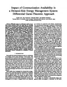
0 Network

IDS (Stop, Continue)

1

False alarm: unit cost

Infection Cost

Virus Shows up at random time

(a) Worm Propagation model Fig. 5.

(b) Markov Chain model for the analysis

Worm propagation model and the the Markov chain model.

2.4

14 λ =5 0

α=1000, µ=.1, γ=.2

λ =10

2.2

12

0

λ =15 0

10 Infection cost

Virus Gain: Linear

2

1.8

1.6

6

1.4

4

1.2

2

1

0

20

40

60

80

0

100

λ (/sec)

(a) Monte Carlo simulation of the exponential infection cost as a function of the worm’s propagation rate Fig. 6.

8

0

200

400 600 Worm’s Propagation rate (β)

800

1000

(b) Worm infection cost as a function of the propagation rate

Cost of security as a function of the virus propagation rate

the name of Intrusion Prevention System (IPS). In practice, an IPS requires inserting a short delay into the system, say 40ms, which not all network designers might like. A related paper is [8]. However their model is substantially different since the virus propagation rate is known and the computer is either infected at time 0 or never infected. Moreover, in that paper, the IDS lets the traffic through even when its volume exceeds the detection threshold. For such a system, it is not difficult to show that the infection cost increases with β so that the optimal strategy for the attacker is to choose the most aggressive virus. We consider a SIS (Susceptible-Infected-Susceptible) virus spreading model ([9],[4]). In such model, a computer is first susceptible once a new virus appears. Then, eventually, the machine will get infected, and after cleaning it becomes again susceptible. A discrete version of such model is shown is figure 5(b). SIS models have been widely used in viral epidemiology [10], and computer virus propagation [4]. Although it is not always realistic (a more realistic model would be Susceptible-Infected-Recovered SIR), SIS models offer a nice analytical framework. Interested readers are referred to [9]. We evaluate the infection and the inspection costs of the

model using a discrete time Markov chain model with time step T of the security system. The states are 0 and 1 where 0 means that the computer is not infected and 1 that it is. Let p0 = P [Xn > x| No Virus] designate the probability that the IDS declares that the computer is infected when it is not (false alarm) and p1 = P r[Xn > x| Virus] the probability that the IDS declares that the computer is infected when it actually is (correct detection). Finally, let µ be the probability that the computer gets infected in one time step. Figure 5(b) shows a diagram of the Markov chain. The transition probabilities of the Markov chain are then P (0, 1) = µ and P (1, 0) = p1 . Also, when the system is in state 0, it generates a false alarm with probability p0 and this false alarm has a unit cost. When the system is in state 1, it generates an average number of viruses equal to β(1−p1 ) and we assume that each released virus has an average cost equal to γ. Thus, γ measures the likelihood that a released virus is successful in infecting another computer. (More complex models are certainly plausible.) With this model, the average cost per unit of time is C = p0 π0 + γβ(1 − p1 )π1 where π0 (resp. π1 ) is the stationary probability that the

833


µ 0.01 0.01 0.01 0.10 0.10 0.10

γ 0.02 0.05 0.10 0.02 0.05 0.10

β 150 220 250 250 150 90

TuB06.6

6

x 980 900 750 580 310 180

the threshold x equal to the Nash Equilibrium value xN E , the infection cost Cost(β, xN E ) is always less than the NE cost Cost(βN E , xN E ).

TABLE II NASH EQUILIBRIUM (β, x) AS A FUNCTION OF THE PARAMETERS (µ, γ).

system is in state 0 (resp,. 1). The stationary distribution can be computed by solving the equations: µπ0 = p1 π1 ,

and

π0 + π1 = 1

Consequently, C=

p0 p1 + β(1 − p1 )µ . p1 + µ

We analyze this model by assuming that Xn is uniform in [0, α] when the computer is not infected and uniform in [β, α + β] when the computer is infected (i.e., the virus is introducing additional traffic of constant rate β). We find that there is a unique Nash equilibrium (β, x) [7]. This Nash equilibrium depends on the values of µ, α, and γ. Table II shows some representative values when α = 1000. Next, we analyze how the infection cost depends on the strategy of the virus. For comparison purposes, we first plot in 6(a), the average cost of the IDS in [8] as a function of the propagation rate of the worm. We omit the details of the analysis and refer the reader to the paper. As can be seen in the figure, the infection cost in an increasing function of the virus’s propagation rate. This tells that the more aggressive a worm is, the more damage it will cause to the system the extreme case being a virus that can user the whole channel. Of course, there are some natural limitations to the rate at which a worm can propagate (finite channel bandwidth but more fundamental is the random scanning that worms use). Worms cannot get around limitations due to finite channel bandwidth, however, other limitations (such as random scanning) can be overcome by very sophisticated viruses. The infection cost, in the model described in this paper, is shown in figure 6(b). As can be seen, with this model, aggressive worms will cause less damage. Actually, they will be detected at the IDS level and will not make it through the system. We do not observe this with traditional IDS because they essentially have an observation window, which delays the detection time. It is during this observation window when aggressive viruses can cause large damage by sending at arbitrary rate. Our model overcomes this by delaying the communication of (eventually) normal users. This is certainly a limitation of the model. However, using this model, one can guarantee a certain level of security independently to how aggressive the attackers are. By setting

IV. C ONCLUSION AND F UTURE W ORK In this paper we analyze two game-theoretic models of network security. In the first model, an intruder may be present and able to corrupt the messages that the network transports. We analyze the Nash equilibria for the intruder and the user of the messages. We show that if the user has the possibility of testing the messages for validity at a small cost and punish an intruder when detected by recovering this cost, this threat reduces the likelihood of attacks enough to make the network trustworthy. In the second model, we analyze the design of a virus aggressiveness level and of an intrusion detection system. We find that by buffering traffic before letting it propagate and potentially infect other computers, the system forces the virus designer to limit the virus aggressiveness, thus reducing the infection cost. In future work, we plan to analyze the benefits of collaborative virus detection and more sophisticated network protection schemes.

Acknowledgments We thank Vern Paxson and Shachar Kariv for their useful comments for the security and game theoretic aspect of the work. We also wish to thank Venkat Anantharam, Marc Felegyhazi, Libin Jiang, Jiwoong Lee, John Musacchio, Galina Schwartz, and Nikhil Shetty for their constructive suggestions. This work is supported in part by NSF under Grant NeTSFIND 0627161. R EFERENCES [1] T. Miller, “Social Engineering: Techniques that can bypass Intrusion Detection Systems,” June 2000, availale at http://www.stillhq.com/pdfbd/000186/data.pdf. [2] K. D. Mitnick and W. L. Simon, The Art of Deception: Controlling the Human Element of Security. New York, NY, USA: John Wiley & Sons, Inc., 2002. [3] S. Lineberry, “The human element: the weakest link in information security.” 2007, availale at http://www.aicpa.org/pubs/jofa/nov2007/human_element.htm. [4] G. Serazzi and S. Zanero, “Computer virus propagation models,” 2003. [Online]. Available: citeseer.ist.psu.edu/serazzi03computer.html [5] M. J. Osborne and A. Rubinstein, A Course in Game Theory. MIT Press, 1994, ch. 1. [6] D. Fudenberg and J. Tirole, Game Theory. MIT Press, 1991, ch. 6. [7] A. Gueye and J. Walrand, “Communication security: A game theoretic approach,” Tech. Rep., 2008. [Online]. Available: http://www.eecs.berkeley.edu/˜agueye/NetSecGame08.pdf [8] R. A. M. Jaeyeon Jung and V. Paxson, “On the adaptive real-time detection of fast-propagating network worms.” [9] L. Billings, W. M. Spears, and I. B. Schwartz, “A unified prediction of computer virus spread in connected networks,” Physics Letters A, vol. 297, no. 3-4, pp. 261–266, 2002. [10] S. Goldman and J. Lightwood, “Cost optimization in the sis model of infectious disease with treatment,” Topics in Economic Analysis & Policy, vol. 2, no. 1, pp. 1007–1007, 2002.

834