sediment delivery ratio, SDR{, of each morphological unit, i, into which a basin is ... network to a basin outlet, can be carried out using an erosion model and a.
Hydrological Sciences -Journal- des Sciences Hydrologiques,40,6, December 1995
703
Sediment delivery processes at basin scale VITO FERRO Istituto di Genio Rurale, Facoltà di Agraria, Università di Reggio Calabria, Piazza S. Francesco 4, 1-89061 Gallina di Reggio Calabria, Italy MARIO MINACAPILLI Dipartimento ETTA, Facoltà di Agraria, Università di Palermo, Viale dette Scienze, 1-90128 Palermo, Italy Abstract Since eroded sediments are produced from different sources distributed throughout a basin, sediment delivery processes at basin scale have to be modelled by a spatially distributed approach. In this paper a new theoretically based relationship is proposed for evaluating the sediment delivery ratio, SDR{, of each morphological unit, i, into which a basin is divided. Then, using the sediment balance equation written for the basin outlet, a relationship between the basin sediment delivery ratio, SDRW and the SDRt is deduced. This relationship is shown to be independent of the soil erosion model used. Finally, a morphological criterion for estimating a coefficient, /3, is proposed. Les processus d'apport de sédiments à l'échelle du bassin versant Résumé Comme les sédiments sont produits dans différentes zones (sources des sédiments) réparties à travers un bassin versant, les processus d'apport de sédiments qui se déroulent dans ce bassin versant doivent être simulés par un modèle mathématique utilisant des données réparties dans l'espace. Dans la présente étude, les auteurs proposent d'abord une nouvelle équation théorique permettant d'estimer le coefficient de production de sédiments SDR( de chacune des unités morphologiques selon lesquelles le bassin versant a été divisé. Ensuite, en utilisant l'équation de bilan des sédiments relative à l'exutoire du bassin, les auteurs établissent une relation entre le coefficient d'apport de sédiments du bassin versant SDRW et le coefficient SDR{. On peut démontrer que cette relation est indépendante du modèle mathématique utilisé pour estimer l'érosion. Enfin, un critère morphologique est proposé pour estimer un coefficient, (3. INTRODUCTION The prediction of sediment yield, i.e. the quantity of sediments which is transferred, in a given time interval, from eroding sources through the channel network to a basin outlet, can be carried out using an erosion model and a mathematical operator which expresses the sediment transport efficiency of the hillslopes and the channel network (Renfro, 1975; Kirkby & Morgan, 1980; Walling, 1983). This mathematical operator can be complex and represent, for each sub-area into which the basin is divided, the balance between the sediment transport capacity of the flow and the sum of the upstream sediment yield and Open for discussion until I June 1996
704
V. Ferro & M. Minacapilli
soil erosion by raindrop impact and runoff (Meyer & Wischmeier, 1969). In contrast, the sediment lag between sediment yield and erosion can be simply represented by the sediment delivery ratio. The basin sediment delivery ratio, SDRW is the fraction of gross erosion (interill, rill, gully and stream erosion) that is expected to be delivered to the outlet of the drainage area considered. SDRW is dependent on the drainage area and other basin characteristics as described by relief, stream length, bifurcation ratio, the proximity of the sediment source to the stream, and the texture of the eroded material (Renfro, 1975; Bagarello et al., 1991). Sediment delivery ratio equations have been developed from studies of basins located in particular regions. Their predictive ability is therefore limited to these regions (Kent Mitchell & Bubenzer, 1980). For this reason SDRW values reported in the literature for given basins and specific time intervals (for example, the mean annual value) can vary from 0.1 to 100% (Walling, 1983). Sediment delivery ratios generally decrease with increasing basin size, indexed by area or stream length, and ASCE (1975) suggested the use of the following power function: (1)
SDRW = kS:
in which k and n are numerical constants and Sw is the basin area. Figure 1 shows some regional relationships, having the mathematical shape of equation (1), for which the exponent n varies between -0.01 and —0.25. The noticeable variability of SDRW for a given Sw value is due to the influence of local factors. For example, the SDRW values measured for Blackland Prairie, Texas, USA (Maner, 1962) are greater than those measured for other American basins. This difference probably depends on the high clay content of the soils in the Blackland Prairie region. The clay particles, transported as suspended load, are generally not deposited along the hillslope conveyance system or in the channel network (Williams & Berndt, 1972). In Fig. 1 the following relationship developed by Bagarello et al. (1991) for the Sicilian region is also plotted: (2)
SDR,., = 5.371S,w-0.6953 ""'•F
Co
'ON SHAANXI CHINA
Fig. 1 Comparison of different relationships between SDRW and basin area
Sediment delivery processes at basin scale
705
in which SDRW is non-dimensional and Sw is measured in km2. The inverse relationship between SDRW and Sw can be explained by the upland theory of Boy ce (1975). According to this theory the steepest areas of a basin are the main sediment-producing zones, and since average slope decreases with increasing basin size the sediment production per unit area decreases too. Large basins also have more sediment storage sites located between sediment source areas and the basin outlet. The sediment delivery ratio is a spatially lumped concept. However, in reality sediments are produced from different sources distributed throughout the basin; each source is characterized by its sediment detachment, transport and storage. Each source area is also characterized by its travel time, i.e. the time that particles eroded from the source area and transported through the hillslope conveyance system take to arrive at the channel network. The dependence of the sediment delivery processes on local factors (sediment detachment, flow transport, travel time, etc.) emphasizes the need to use a spatially distributed approach for modelling this phenomenon. To apply a spatially distributed strategy at the basin scale requires the choice of both a soil erosion model and a spatial disaggregation criterion for the sediment delivery processes. The soil erosion model can be either physically based or parametric. A physically based model involves sub-models which simulate the mechanics of all erosion, deposition and transport processes. This type of model is theoretically preferable but its parameters, which are often numerous, may not be simple to measure or estimate and the scale of measurement may not be at the same level as the scale of the basin discretization for applying the model. For these reasons the parametric approach is the more attractive methodology even if the optimized parameters have no physical meaning since they lump together the effects of several different processes and inaccuracies (Dickinson et al., 1986; Richards, 1993). To use a soil erosion model at the basin scale with spatial disaggregation of the sediment delivery processes requires that the basin be discretized into morphological units (Bagarello et al., 1993),i.e. areas of clearly defined length and steepness (Fig. 2). Such a distributed approach allows for within-basin variability of the sediment delivery ratio and, in particular, takes into account the following circumstances: (a) low slope downstream areas have low delivery ratios (Boyce, 1975); (b) much of the predicted sediment yield is produced in a small percentage of the total basin area; and (c) steep fallow areas near main channels contribute to both erosion and sediment yield while steep row-cropped fields remote from the channel network are characterized by local erosion but contribute little to sediment yield. In this paper, first a theoretically-based expression for the sediment delivery ratio, SDRt, of each morphological unit is proposed. Then, using the
706
V. Ferro & M. Minacapilli
Fig. 2 Example of basin divided into morphological units,
sediment balance equation written for the basin outlet, a relationship between SDRW and SDRt is deduced. Finally this relationship is shown to be independent of the soil erosion model used. THE SEDIMENT DELIVERY RATIO OF A MORPHOLOGICAL UNIT It is hypothesized that the Sediment Delivery Ratio, SDRt, of each morphological area is a measurement of the probability that the eroded particles arrive from the considered area into the nearest stream reach. SDRi is dependent on the travel time, tpJ, of each morphological unit and it is, therefore, assumed to decrease both as the length, / -, of the hydraulic path increases and as the square root of the slope, s -, of the hydraulic path decreases. The probability that the eroded particles arrive from the morphological unit into the nearest stream reach is assumed proportional to the probability of non-exceedence of the travel time, f •. In order to specify the mathematical shape of the relationship between SDRj and / /ys the empirical cumulative frequency distribution function (CDF) of the variable
707
Sediment delivery processes at basin scale
/ t/Js i is required. In order to study the CDF of the travel time, seven Sicilian basins (Fig. 3) were selected. The characteristics of these basins, name, area Sw (km2) and number of morphological units, Nu, are listed in Table 1.
Table 1 Basin characteristics
K
a
Basin Sw Sub-basin (km2)
K
a
368
967
2.40
Raia
201
1.00
Basin Sub-basin
(km2)
Belice sinistro
17
Belice 1
245
439
2.50
Timeto
93
296
1.22
Belice 2
154
317
2.40
Timeto 1
78
249
1.24
Belice 3
92
195
2.40
Timeto 2
62
185
1.28
Belice 4
54
103
2.80
Timeto 3
49
159
1.27
Belice destro
44
90
1.90
Timeto 4
39
123
1.07
Elicona
56
298
0.80
Timeto 5
30
99
1.10
Elicona 1
9
55
0.70
Timeto 6
23
67
1.14
Elicona 2
18
114
0.77
Timeto 7
17
49
1.32
Elicona 3
37
191
0.70
Timeto 8
13
40
1.38
Elicona 4
45
244
0.90
Timeto 9
8
35
1.06
Fastaia
40
133
2.40
Timeto 10
7
22
1.40
Imera mer.
27
101
1.20
Timeto 11
2
8
1.00
-#
FASTAIA
fits,.
o La C h l n * a
BELICE DESTRO a Piana degli AIDanesi BELICE SINISTRO o Garcia RAIA a P r i z z i IMERA
MERIDIONALE a
Petrolia
ELICONA TIMETO
Fig. 3 Sicilian basins investigated in this research.
708
V. Ferro & M. Minacapilli
Figure 4 shows that for the selected basins, the relationship between the logarithm of the cumulative frequency Fh lnF;, and the variable —lilJsi is linear for each basin. Consequently, the following relationship can be assumed for evaluating SDRt: (6)
p,i
SDRt = exp(-j8f •) = exp
in which (3 is a coefficient which is assumed constant for a given basin, since the relationship between InF, and —tp t is linear (Fig. 4).
0.00 •
1
BKI-ICKS1N.
—
-1.00 D BEL1CE DES.
-2.00
•
y|
ELICONA
O FASTAIA
• •
-3.00 A IMERAMER
•
•
lu Ki
•
A RA1A
-4.00
•
_i-rd
•
TIMEÏO
_
^ Q
;f
A
•
f
** S A A
•
•
"J
wf
~~5
a
-7.00 -16000
14000
-12000
-10000
-8000
-6000
-4000
-2000
l
- P,i
Fig. 4 Cumulative frequency plots of —l./Js basins
. for the seven Sicilian
For evaluating the travel time of the particles eroded from a given morphological unit i, the travel times of all morphological areas which are localized along the path between the z'th unit and the nearest stream reach have to be summed. This gives: p>t
= I-
X:V
(4)
7-1 P,i
V N
in which Np is the number of morphological units localized along the hydraulic path, and X( and stj are the length and slope of each of they morphological areas. Equation (3) can now be rewritten in the following form:
Sediment delivery processes at basin scale
709
N
SDRt = exp
" hi
I-
(5)
lJ
J=1.
RELATIONSHIP BETWEEN BASIN SEDIMENT DELIVERY RATIO AND SDR{ In order to evaluate the /3 coefficient of equation (5), a sediment balance equation for the basin outlet has to be written. The balance equation establishes that the sediment production for the basin outlet, Ps (t), is equal to the sum of the sediment produced by all morphological units into which the basin is divided: N„
N„
^SDRiA^i
l = £exp -0. PJ
A:lS, U,l
(6)
where At is the soil loss (t ha"1) from a morphological unit which can be estimated by a selected erosion model (USLE, RUSLE, etc.), SuJ is the area (ha) of the morphological unit and Nu is the number of morphological units into which the basin is divided. To apply equation (6), a soil erosion model at the plot scale has to be selected and measurements of Ps are necessary. The sediment balance equation is based on the hypothesis that the sediment production (SDRt At SuJ) which arrives from a given morphological unit or sediment source into a stream reach can be transported to the basin outlet. This hypothesis agrees with Playfair's law of stream morphology which states that over a long time a stream must essentially transport all sediment delivered to it (Boyce, 1975). In other words it is hypothesized that the transport capacity of the river flow, Tc, is not a limiting factor; i.e. Tc is always greater than the actual sediment transport which is equal to the hillslope sediment yield, Th, An alternative hypothesis is that the /3 coefficient is used to calibrate the model and to take into account the possible case that Th > Tc. Referring to the mean annual value, sediment production can be expressed as the product of SDRW and the basin soil loss, Aw (t). By using the Universal Soil Loss Equation (Wischmeier & Smith, 1965) for estimating Aw, equation (6) can be rewritten in the following form: Nu
£exp -0-
L
RiKMqp&j
(=i
(7)
SDR,.
ZR^L^qp^
710
V. Ferro & M. Minacapilli
in which Rt is the rainfall erosivity factor of the z'th morphological unit; Kt is the soil erodibility factor; £ $ is the topographic factor; C; is the cover and management factor; and P( is the support practice factor. If the basin is divided into morphological units and the factors of the USLE equation are estimated for each morphological unit, equation (7) can be used to deduce the relationship between SDRW and the j3 coefficient of equation (3). For the basins studied, the relationship SDRW = $((3) will allow one to calculate the coefficient /3 corresponding to a SDR,» value which can be estimated by available relationships such as equation (1) (Glymph, 1954; Roehl, 1962; Williams, 1977; Walling, 1983; Bagarello et al, 1991). Figure 5 shows, for the Timeto basin, values of /S and SDRW calculated with equation (7), using SDRW values ranging from 0 to 1, and the fitted relationship: SDRW = exp(-1000a/3)
(8)
in which a is a constant estimated by least squares.
1
1
°
cq.(7) "1 •
c>
i3
C
1000 ft
Fig. 5 Values of basin sediment delivery ratio and /3 for the Timeto basin.
In order to test whether equation (7) is independent of the selected relationship for calculating the topographic factor, Lph the relationships used in the RUSLE (Renard et al., 1994) and in the WEPP models (Moore & Wilson, 1992) were also applied. For the RUSLE model, the topographic factor has the following expression:
L-S= i"i
L-S= ^iui
\
22.13
\
22.13
(10.8 sina,. + 0.03)
if tana- < 0.09
(16.8 sina;. - 0.05)
if tana- > 0.09
(9a)
(9b)
in which \ is the slope length of the ith morphological area and ai is its slope angle, mi = ^ / ( l + fi), and/J- = sina//0.0896(3sin°-8a/ + 0.56).
Sediment delivery processes at basin scale
111
The second method for calculating LiSi was proposed by Moore & Burch (1986), and is also used for the WEPP model. It is given by: 1.3
0.6
M/
(10)
sma 0.0896
22.1
in which Asj is the. ratio between the area of the morphological unit and the width measured along the contour line. Figure 6 for the Timeto basin clearly shows that equation (7) is independent of the selected procedure for calculating
Lfi. is
1
9
•
3
1 1 OSLE
O RUSLE
9
0.6
• MOORE ft BURCH
0 5
SDRw 0.4
%1 5 i '•
0
1
2
3
1
5
4s
i!
ii
•
4
6
7
i1 8
S
9
1000 p
Fig. 6 SDRW values calculated by equation (7) and different methods of estimating the topographic factor.
Equation (7) can be simplified if it is hypothesized that the basin sediment delivery ratio can be calculated, by using only morphological data, from the following relationship:
lexp
-is-lpJ
i=l
rp,i
SDRm =
L S S
i i u,i
(11)
i=l
Equation (11) shows that the basin morphological sediment delivery ratio, SDRm, is the weighted mean of SDRt values, with a weight equal to LiSiSu,-. Figure 7 shows the comparison between SDRm and SDRW values for selected basins. These plots, showing that the pairs (SDRW, SDRm) are very near to the line of perfect agreement, demonstrate that equations (7) and (11) are equivalent within the studied region. In order to test whether the relationship between the basin sediment delivery ratio and the @ coefficient is independent of the selected erosion model, SDRW values calculated by equation (7) were compared with SDRM values calculated by the following relationship:
V. Ferro & M. Minacapilli
712
Eexp
- ^
S S
\
1=1
i uJ
(12)
SDRM = M EX«
s S
i u,i
in which s( is the slope of the ith morphological unit. Equation (12) is deduced from equation (11) after hypothesizing, according to Wischmeier & Smith (1965), that the Lt factor of the ith morphological unit is proportional to the square root of the slope length and that the S factor is proportional to s\.
~JnBEI.ICRDBS. z z i _ LJ "
(a)
*r
•
M
,
HMRTO
|
/"'"
0.6
^1 (b)
•l1
| 1
EUCONA
e o.6
L-^'
y j
|
(d)
|
m-
et O m
1 "^ •