Segmentation of color images by clustering 2D histogram and merging regions Olivier Lezoray1 , Hubert Cardot2 1 LUSAC, IUT SRC, 120, Rue de l’exode, 50000 Saint-Lˆo, France 2 LI EA 2101, Dept. Informatique, Polytech Tours, 64 Avenue Jean Portalis, F-37200 Tours, France E-mail:
[email protected] [email protected] R´esum´e Une m´ethode hybride de segmentation d’images couleur est pr´esent´ee dans cet article. Dans une premi`ere e´ tape plusieurs histogrammes 2D sont partionn´es et les cartes de r´egions correspondantes sont fusionn´ees. Ceci permet d’obtenir un premier partionnement grossier de l’image par rapport a` ses couleurs dominantes. L’information couleur attach´ee a` chacune des r´egions est ensuite utilis´ee dans une deuxi`eme e´ tape. Une nouvelle technique de simplification du Graphe d’Adjacence des R´egions est propos´ee en proc´edant par la fusion de r´egions deux a` deux jusqu’`a la stabilisation d’un crit`ere d´efinissant la pertinence de la segmentation. Les r´egions finales obtenues apr`es fusion sont ensuite affin´ees au niveau de leurs contours par l’utilisation d’une ligne de partage des eaux utilisant les propri´et´es locales et globales de l’image. La robustesse de la m´ethode est exp´erimentalement e´ prouv´ee sur une base d’images et l’influence des diff´erents param`etres e´ tudi´ee.
Mots-cl´es Couleur, Partitionnement, Ligne de Partage des Eaux, Graphe d’Adjacence de R´egions, Fusion de r´egions
Abstract An hybrid segmentation method for color images is presented in this work. It combines 2D histogram clustering to produce segmentation maps fused together providing an initial unsupervised clustering of the dominant colors of the image. Region information is then used and a novel technique is introduced to simplify the Region Adjacency Graph by merging candidate regions until the stabilization of a ”good” segmentation criterion. Merged regions are refined by a color watershed
using local and global properties of the image. The robustness of the method is experimentally verified and the color space influence is studied.
Keywords Color, Clustering, Watershed, Region Adjacency Graph, region merging
1
Introduction
Color image segmentation refers to the partitionning of a multi-channel image into meaningful objects [Ohta et al., 1980]. With the growing of digital image databases, efficient segmentation methods are needed for extracting and coding image regions. Various approaches can be found in the litterature and can be roughly classified into several categories: clustering methods [Littman and Ritter, 1997, Campadelli et al., 1997], edge-based methods [Zugaj and Lattuati, 1998], region growing methods [Tr´emeau and Borel, 1998, Schettini, 1993], morphological watershed based region growing methods [Belhomme et al., 1997, Saarinen, 1994, Shafarenko et al., 1997]. Many of the existing segmentation techniques, such as supervised clustering use a lot of parameters which are difficult to tune to obtain a good segmentation [Cappellini et al., 1995]. By good segmentation we mean that the image has been partitionned into homogeneous colored regions. A new approach of segmentation is proposed towards this goal. This approach minimizes the number of parameters to one multi-scale parameter and acts as an unsupervised method. We propose to combine different types of methods to obtain a final segmentation of a color image. The basic idea of the segmentation is to divide the segmentation process into three stages: color clustering, region merging and watershed segmentation. In the first stage, 2D histograms are used to obtain a rapid and coarse clustering of the color image. This clustering provides three segmentation maps which are fused together giving the final segmentation map of the clustering. This clustering is fast, simple and unsupervised (the number of classes is automatically estimated with morphological operators). This segmentation map is however over-segmented and the second stage proceeds to a region merging of adjacent regions until the stabilization of a criterion for the segmentation. This criterion is based on an extension of the definition proposed by Liu [Liu and Yang, 1994] and involves the minimization of a cost associated with the partitionning of the color image. The merging of similar adjacent regions is therefore iteratively and automatically performed [Garrido et al., 1998]. In the third stage, a segmentation refinement is based on a modified color watershed using local and global color criteria [Lezoray and Cardot, 2002]. The three-stages segmentation enables to consider in the first stage the spatial distribution of the colors to cluster the image and in the next two stages the color similarity between regions and pixels or regions. This is similar to a focus of attention: in the first stage homogeneous colored regions are retrieved, merged according to their color similarity and refined according to their local color neighborhood. The organization of the paper is as follows. In section 2 the clustering of an image with a 2D histogram clustering
and fusion is discussed. In section 3, the region merging strategy is detailled. In section 4 the watershed segmentation is presented. The results obtained with the proposed method are presented and discussed in section 5.
Figure 1: The 3D RGB histogram of the figure 6(b).
2
2D histogram clustering and fusion
To perform a clustering of a color image, several strategies can be employed. The strategies generally differ on the dimension of the data used to cluster the image. In the 1D case, the histograms of each band are considered separately and the method is reduced to finding thresholds dissecting the band histograms [Celenk, 1990, Lezoray and Cardot, 2002]. This method relies on the fact that the objects in the image give rise to explicit peaks in the histograms. The resulting segmentation maps can be combined with different methods, such as majority vote, Demspter-Shafer or Bayesian theory. This method is known as multithresholding. In the 3D case, the vectorial aspect of color is taken into account and the clustering is considered as the classification of multispectral data. The spatial repartition of the colors in the associated color space is used to cluster the image assuming that the colors of the objects are grouped around dominant colors in the 3D histogram [Soille, 1996, Park et al., 1998, Postaire et al., 1993, G´eraud et al., 2001] (the center of the classes). Both 1D and 3D methods suffer from the determination of the number of classes, which is usually assumed to be known. The 1D method also suffers from the fact that a color cluster is not always present in each band and the combination of the different segmentations cannot catch this spatial property of the colors. The 3D method is handicapped with data sparseness on the one hand (see figure 1) and with the complexity of the search algorithm on the other hand.
2.1
2D color histogram
An interesting alternative to these two methods lies on the use of partial histograms [Kurugollu et al., 2001] (2D histograms) which use two color bands to-
gether namely RG, RB and GB in the RGB color space. This can bring several advantages. The paucity of the data encountered in the 3D case is partially overcame and the search complexity is drastically reduced. Moreover it partially uses the spatial repartition of color and offers an intermediate method to the 1D and 3D ones. Another advantage to be considered is the fact that a 2D histogram is nothing more than a grey-level image, therefore classical and fast grey-level image processing algorithms can be used to cluster the 2D histogram.
2.2
Unsupervised morphological clustering
In this section we propose a new method for clustering 2D histograms obtained from color images. A 2D histogram is the projection of a 3D histogram onto band-pair planes (see figure 2(a)). To cluster this 2D histogram, we assume that the different objects of the image are present in the histogram around the dominant peaks (homogeneous regions in this grey-level image). Obviously these peaks also correspond to peaks in the 3D case. The main peaks of the 2D histogram are considered as the cluster centroids. The main difficulty is to find the peaks whithout a priori knowledge on their number. The method we propose is based on a morphological clustering of the image. Morphological operators are simple, fast and have proved their abilities in processing grey-level images [Serra, 1982, Park et al., 1998, Postaire et al., 1993]. The clustering of the 2D histogram proceeds in several steps. Since the histograms are generally noisy (this is mainly due to the sparseness of the colors in the images), the latter is smoothed with a symetrical exponential filter (with a given parameter β ∈ [0, 1]) and the result is reconstructed in the original image to obtain a noiseless and regularized version of the histogram (see figure 2(b)).
(a) The inverted RG 2D histogram of the figure 6(b).
(b) The reconstructed image of the image 2(a).
Figure 2: A 2D histogram. To accelerate the cluster centroids determination, the smoothed histogram (of 256x256 size) is reduced to 128x128 by a down-sampling of factor 2. The downsampling is done by giving to each bin the mean value of the considered neighbor-
hood (see figure 3(a)).
(a) The image 2(b) down-sampled by a factor 2.
(b) The dominant colors of the image 3(a).
Figure 3: Extraction of the dominant colors. The main peaks correspond to maxima in the 2D histogram, therefore an erosion applied on the latter reduces each bin to its main colors. This property is used to extract the dominant colors. From this reduced histogram, the ultimate erode set is extracted giving the main dominant colors of the 2D histogram. This method directly extracts the color cluster centroids whithout any assumption on the number of classes: the centroids are considered to be the pixels which lastly disapear in an iterative process of morphological erosions (namely the ultimate erode set, see figure 3(b)). These centroids are labelled (see figure 4(a)) and a Voronoi partitionning of the 2D histogram is performed providing the clustering of the histogram. The clustered histogram is finally up-sampled to its original resolution (256x256) by replication of the labels (see figure 4(b)).
(a) The labelled image of the image 3(b).
(b) The Voronoi partitionning of the image 4(a).
Figure 4: Clustering of a 2D histogram. From the clustered 2D histogram a segmentation map is obtained since each region in the histogram image corresponds to a set of colors in the original image: to each (RGB) vector is associated the corresponding label in the clustered 2D histogram (see figure 5(a)).
2.3
Fusion of segmentation maps
The above clustering method is applied to the three 2D histograms obtained from a color image and three different segmentation maps are obtained. The resulting segmentation maps have to be combined all together to provide the final clustering of the image. Since the 2D histograms are processed independently, there is no guarantee that the same label will be assigned to a same type of cluster in the different segmentation maps (the assignment of the labels is arbitrary). Moreover, each 2D histogram may distinguish a number of regions which can be different from a 2D histogram to another since they do not contain the same information. For each segmentation map of RG, RB and GB, the set of regions is denoted by E(S) where S is a segmentation map (see figures 5(a)-(c)). According to the previous step, for each segmentation map Si , ∀i ∈ {RG, RB, GB}, we can associate a number of regions Θ0 (Si ) = Card(E(Si)). The fusion of the three segmentation maps is made in a very simple way: the final set of regions is deduced from the superimposition of the different region sets E(SRG ), E(SRB ), E(SGB ) [Lezoray and Cardot, 2002].
(a) The segmentation map of the RG 2D histogram.
(b) The segmentation map of the RB 2D histogram.
(c) The segmentation map of the GB 2D histogram.
(d) The superimposed segmentation map.
Figure 5: Superimposition of segmentation maps.
The superimposition produces a new image of labels (denoted by SRGB ) which is compatible with all the segmentation maps of the color planes (see figure 5(d)). The number of regions of SRGB is deduced from the intersection of the different regions of the three segmentation maps with the following property: Θ(SRGB ) ≥ max(Θ(SRG ), Θ(SRB ), Θ(SGB )). A majority filter is finally applied to the resulting image SRGB to obtain the final segmentation map. The majority filter gives to each pixel of SRGB the most frequently encountered label in a 3x3 neighborhood. This operation suppresses isolated pixels which are incorporated into the larger adjacent region and filters the remaining local label uncertainties on noisy or textured zones (see figure 6(a)). One can state that the final regions extracted correspond to homogeneous regions in the original color image (see figure 6(b)). If the main color of each region is associated to each pixel of these regions, a quantized image of the original image is obtained. The parameter β used to smooth the 2D histograms acts as a multi-scale parameter. It defines the level of dominant colors to be preserved by the clustering. The figures 7 illustrate this property. For each one of these images, the final number of color decreases with β: it corresponds to light towards strong regularization of the 2D histograms. This number of colors is equivalent to the number of regions in the resulting segmentation map. The initial number of colors in the original color image is 24581 and decreases with β (see figures 7 and 8). In this paper β has been fixed at 0.35 by extensive experimentations on image databases.
(a) The final segmentation map after the majority filter.
(b) The original color image used for segmentation.
Figure 6: Segmentation map after the first step of the proposed method.
3
Region merging
Given the initial image clustering which defines an image segmentation (often oversegmented), a merging strategy is needed to join the most coherent adjacent regions together. The data structure used to represent the region partition of the image is the Region Adjacency Graph (RAG). We propose to use a RAG to simplify
(a) β = 0.1 (280)
(b) β = 0.35
(422)
(c) β = 0.6 (923)
(d) β = 1.0
(1788)
Figure 7: Quantized images with different values for β, the number in brackets gives the number of colors in the image. the initial image segmentation by merging adjacent regions.
3.1
RAG construction
A RAG is a set of nodes representing connected components (the regions) of the image and a set of links connecting two neighboring nodes [Saarinen, 1994, Shafarenko et al., 1997, Morris et al., 1986, Haris et al., 1998, Garrido et al., 1998, Makrogiannis et al., 2001]. This RAG denoted by G = (V, E) is constructed to describe a partition of the image by the topology and the inter-region relations of the image. It is defined by an undirected graph where V = {1, 2, ..., K} is the set of nodes and E ⊂ V × V is the set of edges (links between adjacent regions). K = Θ(G) is the number of region nodes. Each edge is weighted by a value indicating the similarity between two adjacent regions. The most similar pair of adjacent regions corresponds to the edge with the minimum cost. A merging algorithm on the RAG uses this property to merge region nodes corresponding to edges of minimum cost. This cost associated to each edge is therefore very important in order to define which regions will be merged. A merging algorithm on a RAG is therefore a technique that removes some of the links and merges the
Figure 8: Variation of the number of quantized colors (i.e. the number of regions) according to β corresponding nodes. The algorithm is simple: the pair of most similar regions are merged until a termination criterion is reached. For a complete merging strategy based on a RAG, several notions have to be defined [Garrido et al., 1998, Salembier and Garrido, 2000, Salembier et al., 1997]: ➀ The region model: when two regions are merged, the model defines how to represent the union. This model is denoted by M (R). ➁ The merging order: it defines the order in which the links are studied to know whether or not they should be used for merging. This order O(R1 , R2 ) associates a value to each pair of adjacent regions according to their similarity. ➂ The merging termination: each pair of adjacent regions is merged until the assessment of a termination criterion. To define our own RAG based merging algorithm, we have to define each one of these three notions.
3.2
Region model
The region model defines how regions are represented and how to represent the union. Each region R has a model M (R) of four values : the RGB vector (summed over each component) and the number of pixels of the region. The merging of two regions R1 and R2 is computed as follows: MR1 ∪R2 = (MR1 + MR2 )
(1)
This allows fast implementation since the union model is directly computed from the models of the two merged regions.
3.3
Merging order
The merging order is based on a measure of similarity between adjacent regions. At each step the algorithm looks for the pair of most similar regions (the edge of minimum cost). The similarity between two regions R1 and R2 is defined by the following expression [Salembier and Garrido, 2000, Salembier et al., 1997]: O(R1 , R2 ) = N1 kMR1 − MR1 ∪R2 k2 + N2 kMR2 − MR1 ∪R2 k2
(2)
where N1 and N2 are the number of pixels of the regions R1 and R2 . M (R) is the region model and k.k2 is the L2 norm. This function O(R1 , R2 ) defines the order in which the regions have to be processed: the regions that are the more likely to belong to the same object. At each edge ER1 ,R2 is associated the value O(R1 , R2 ). Since at each merging step the edge with the minimum cost is required, the appropriate data structure to handle the edge weights is a hierarchical priority queue. Each edge node is inserted in the hierarchical queue at the position defined by the merging order. An interesting representation of the hierarchical queue is a balanced binary tree which is very efficient for managing a high number of nodes with fast access, insertion and deletion.
3.4
Merging termination criterion
The figure 9 gives an overview of the general scheme of the merging process [Garrido et al., 1998]. Given the initial segmentation, the RAG and the hierarchical queue are initialized. Each region is initialized by computing its model and the hierarchical queue is initalized by adding the edge weights into according to the merging order. At each merging step the edge with the minimum cost is removed from the hierarchical queue and the information associated to both regions having to be merged are updated in the RAG structure and in the hierarchical queue. The merging process is iterated until a termination criterion is reached. This termination criterion is a crucial point of the algorithm and defines when the merging ends. Usually this criterion is based on a priori knowledge: the number of regions, the PSNR or other subjective criteria involving threshods. Ideally, for an automatic segmentation, the termination criterion should be based on image properties which define the fact that the segmentation obtained is considered as ”good”. To assess this fact, we have defined a new criterion (based on the one developed by Liu [Liu and Yang, 1994, Borsotti et al., 1998]) using the merging order and the image model to define if the segmentation of an image is considered as ”good” as compared to another one. The segmentation evaluation provides a value which decreases the better the segmentation is. Therefore merging regions gives a better representative segmentation and the evaluation criterion decreases. The edges of the hierarchical queue are processed one by one until a stabilization of the segmentation evaluation criterion. Once a plateau is reached, the segmentation is considered as enough good and representative of the original image (so
that the termination criterion is reached giving end to the merging process). The segmentation evaluation F is defined by the following expression: p Θt (G) F (G, I) = × 1000 × h × w Θt (G) Θt (G) Θt (G) 2 X X X e i Ej,k (3) + 1 + log(N i) j=1 i=1 k>j
where G denotes the graph and θt (G) the number of nodes of G at a given iteration t. I is the initial color image, h, w are respectively the height and the width of I, Ni is the number of pixels of the region number i, Ej,k is the edge weight between the regions j and k (defined only for adjacent regions, 0 otherwise). All the more, each edge weight is added only once. e2i is the euclidean distance between RGB color vectors of the pixels of the ith region and the color vector attributed to the ith region in the segmented image. The smaller the value of F the better the segmentation should be. This can be easily explained. If the segmentation is good, each segmented region has an homogeneous mean color as compared to the original color vectors, this is equivalent to an intra class distance. Moreover the merging of two adjacent regions (wich are of similar colors) makes smaller the sum of the edge weights, this is somehow equivalent to an inter class distance. Once the segmentation evaluation function appears to be stabilized, a tradeoff between the homogeneity of the regions and the difference between the regions has been reached stating that the segmentation is ”as good” as possible: it correctly describes the original image. Merging more adjacent regions will produce a less representative segmentation. An example of merging is given by the figure 10. The original RAG (see figure 10(a)) presents over-segmentation and the merging process reduces it significantly (see figure 10(b)). The final segmentation map is no more over-segmented and always corresponds to homogeneous regions in the original color image (see figures 10 (c) and (d)). The figure 11 illustrates the variation of the F segmentation evaluation criterion. It decreases along the iterations
Figure 9: General scheme of the merging process.
(a) Initial RAG.
(b) Merged RAG.
(c) Final regions.
(d) Quantized image.
Figure 10: Illustrating figures of the merging process until it reaches a plateau ending the merging process. An iteration corresponds to the analysis of an edge link between two regions. To accelerate the processing, the computing of ei is performed in the following way. If two regions R1 and R2 merge then NR1 e2R1 + NR2 e2R2 e2R1 ∪R2 = (4) NR1 ∪R2 This enables a faster implementation of the computing of F (G, I) which is rapidly updated each time two regions merge. A plateau is considered to be reached when a certain number of successive identical values of F is obtained. This number is dependent on the number √ of regions in the original segmentation map and is Θ (G)
0 defined by the quantity where Θ0 (G) gives the initial number of regions 2 before the merging process begins.
4
Color watershed
The extracted regions after the two previous stages are homogeneous but have irregular contours. To avoid this a final stage of the segmentation consists in ap-
Figure 11: Variation of F along the iterations. plying a color watershed to refine the previously extracted regions [Meyer, 1992, Vincent and Soille, 1991, Lezoray and Cardot, 2002, Shafarenko et al., 1997]. The color watershed used in this paper is defined according to a specific aggregation function. The aggregation function defines the aggregating probability of a pixel to a region. It is based on two types of information describing the spatial information of the image: local information expressed by the color gradient and global information expressed by the color mean of the regions describing their color homogeneity. This aggregation function can be formally defined. Let IC1 C3 C3 (R) denote the mean color vector of the region R for the image I in the color space C1 C2 C3 , the I(p) vector giving the color of a pixel p and ∇(p) the color gradient. The aggregation function is expressed as [Belhomme et al., 1997, Lezoray et al., 2000, Lezoray and Cardot, 2002]: f (p, R) = (1 − α)kIC1 C3 C3 (R) − IC1 C2 C3 (p)k+ αk∇IC1 C2 C3 (p)k
(5)
This function combines local information (modulus of the color gradient) and global information (a statistical comparison between the color of a pixel p and a neighbor region R performed with the Euclidean distance). During the growing process, each time a pixel is added to a region R, the mean color of the region is updated. The color image and the gradient image are both normalized before the watershed growing to have values in the same range. α is a blending coefficient which allows to modify the influence of the local and global criteria during the growing process. The gradient is processed using Di Zenzo’s definition [DiZenzo, 1986]. To perform the growing, the contours of the regions are considered as unlabeled pixels but also the pixels of regions smaller than a 3 × 3 structuring element. Usually, α is fixed according to a priori knowledge on the
images. However, an adaptable segmentation which modifies the value of α along the iterations seems more suitable [Lezoray and Cardot, 2002]. The initial value of α is 0 and evolves during P the growing. At each iteration k, the following quantity is computed: Vk = f (p, R) for all the processed unlabeled pixels p. The set of processed pixels is a subset of all the unlabeled pixels of the image and designs only unlabeled pixels adjacent to a given region. Therefore V0 gives the initial value for all the unlabeled pixels of the image processed at the first iteration. These pixels are directly adjacent to the markers. Since the initial value of α is 0, V0 quantifies the initial global similarity between the pixels and the region markers. If the global similarity Vk is small, the unlabeled pixels are very close to the regions and α has to be small to take only the global information into account. On the contrary, if Vk increases, α has to increase to take into account the local information. To fulfill these requirements α is defined by α = Vk /V0 . It is computed after the processing of all the considered unlabeled pixels. However, it is not desirable to have high variations of α between each iterations. The value retained for the next iteration k+1 is considered to be the mean of all the previous values of α (including the new computed one). This enables a smoother evolution of α (see figure 12). The final segmentation obtained by the color watershed is given by Figure 13.
Figure 12: Variation of α along the iterations.
5
Results and discussion
To assess the influence of the different representations of color (i.e color spaces), we have to compare the obtained segmentations in several color spaces. To see if a segmentation is close to the original image, an error metric is needed. The error between the original image and the quantized image (obtained by associating the main color of each region to each segmented pixel) is generally used. The Mean
(a) The segmentation after the watershed.
(b) The original image with the contours of the regions.
Figure 13: The final segmentation in the RGB color space. Square Error (MSE) is therefore considered to evaluate a segmentation. The MSE is defined by h w 1 XX 2 M SE = e (6) h × w i=1 j=1 i A lower value for MSE means lesser error, therefore the lower the MSE, the better the segmentation. The segmentation scheme proposed in this paper was evaluated on 2000 images from Corel Image CDT M database. Figure 14 presents the mean of MSE obtained over all the images of the database with the following color spaces: RGB, XY Z, HSL, I1 I2 I3 , Y IQ, Y U V , Y Ch1 Ch2 , Y Cb Cr , LU V , LAB.
Figure 14: The MSE for the image database in different color spaces.
Two color spaces give roughly the same results and can be considered as the most relevant ones for our segmentation scheme on the Corel database: the Y U V and the Y Cb Cr . The figure 15 shows the segmentation obtained on the image 6(b). This has to be compared with the segmentation obtained in the RGB color space (see figure 13(b)). It can be observed that the segmentation schemes produces results noticeably better in Y U V and Y Cb Cr , however the final number of regions is higher than in the RGB color space. The choice of the most appropriated color space must be done in compliance with the aim of the segmentation. For efficient and accurate segmentation, the color space minimizing the MSE might be chosen. But for compact representation of the image, the color space giving a compromise between the accuracy (low MSE) and the final number of regions might be prefered. The number of obtained regions obviously decreases with β while the MSE increases. One thing to point out is the fact that β is not a strict multiscale parameter : the number of regions has not a monotonous decrease with β. This is mainly due to the region merging step: the more the number of regions in the original segmentation to simplify, the more the size of the plateau of F to be reached. The study of the color space performed in this section was done with a fixed value of the single parameter of the whole method (β = 0.35). This parameter was initially fixed by experiments performed in the RGB color space. But the choice of the color space also depends on this parameter. Three strategies can be considered. The parameter is fixed for all the different color spaces (one value for all), fixed for each color space (one for each) or lastly, determined for each image to be processed (one for each image in a given color space). The last assumption seems more promising since it enables the adapdation of the method according to each image in a given color space. The filtering of the 2D histogram will therefore be adapted to the spatial repartition of the colors in the histogram. One can even consider different values of β for each 2D histogram. All these queries will be further investigated in future works.
(a) The Y U V segmentation.
(b) The Y Cb Cr segmentation.
Figure 15: Segmentations in two different color spaces.
6
Conclusion
In this paper, a color segmentation method was presented. It consists of three stages: 2D histogram clustering and fusion, region merging and color watershed. The first key idea lies on the use of 2D histogram for clustering color images. This approach is fast, unsupervised and produces segmentation maps over segmented but very close to the dominant colors present in the original image. To avoid the over segmentation effect, we proposed a merging region technique based on Region Adjacency Graph until the stabilization of a segmentation criterion. The final stage proceeds to the region boundaries refinements by a color watershed. The good performance of the whole method has been experimentally verified on several color images and the influence of the color space used for the method was studied. One advantage of the method is its single parameter property. This enables a rapid tuning of the method. Future research work is on how to handle the limitations of the segmentation: mainly the choice of the single parameter according to the image and the color space.
References [Belhomme et al., 1997] Belhomme, P., Elmoataz, A., Herlin, P., and Bloyet, D. (1997). Generalized region growing operator with optimal scanning : application to segmentation of breast cancer images. Journal of Microscopy, 186:41– 50. [Borsotti et al., 1998] Borsotti, M., Campadelli, P., and Schettini, R. (1998). Quantitative evaluation of color image segmentation results. Pattern recognition letters, 19:741–747. [Campadelli et al., 1997] Campadelli, P., Medici, D., and Schettini, R. (1997). Color image segmentation using hopfield networks. Image and Vision Computing, 15(3):161. [Cappellini et al., 1995] Cappellini, V., Plataniotis, K., and Venetsanopoulos, A. (1995). Applications of color image processing. In Proceedings of the International Conference on Digital Signal Processing. [Celenk, 1990] Celenk, M. (1990). A color clustering technique for image segmentation. Computer Vision Graphics and Image Processing, 52:145–170. [DiZenzo, 1986] DiZenzo, S. (1986). A note on the gradient of a multi-image. Computer Vision, Graphics and Image Processing, 33:116–126. [Garrido et al., 1998] Garrido, L., Salembier, P., and Garcia, D. (1998). Extensive operators in partition latties or image sequence analysis. Signal Processing, 6(2):157–180.
[G´eraud et al., 2001] G´eraud, T., Strub, P., and Darbon, J. (2001). Color image segmentation based on automatic morphological clustering. In IEEE International Conference on Image Processing, volume 3, pages 70–73. [Haris et al., 1998] Haris, K., Efstratiadis, S., and Maglaveras, N. (1998). Hybrid image segmentation using watersheds and fast region merging. IEEE transactions on Image Processing, 7(2):1684–1699. [Kurugollu et al., 2001] Kurugollu, F., Sankur, B., and Harmanci, A. (2001). Color image segmentation using histogram multithresholding and fusion. Image and Vison Computing, 19(13):915–928. [Lezoray and Cardot, 2002] Lezoray, O. and Cardot, H. (2002). Histogram and watershed based segmentation of color images. In Proceedings of CGIV’2002, pages 358–362. [Lezoray et al., 2000] Lezoray, O., Elmoataz, A., Cardot, H., and Revenu, M. (2000). A color morphological segmentation. In Proceedings of International Conference on Color in Graphics and Image Processing, pages 170–175. [Littman and Ritter, 1997] Littman, E. and Ritter, E. (1997). Colour image segmentation : a comparison of neural and statistical methods. IEEE Transaction on Neural Networks, 8(1):175–185. [Liu and Yang, 1994] Liu, J. and Yang, Y.-H. (1994). Multiresolution color image segmentation. IEEE transactions on Pattern Analysis and Machine Intelligence, 16(7):689–700. [Makrogiannis et al., 2001] Makrogiannis, S., Economou, G., and Fotopoulos, S. (2001). A graph theory approach for automatic segmentation of color images. In International Workshop on Very Low Bit-rate Video, pages 162–166. [Meyer, 1992] Meyer, F. (1992). Color image segmentation. In Proceedings of the International Conference on Image Processing and its Applications, pages 303–306. [Morris et al., 1986] Morris, O., Lee, M., and Constantinidies, A. (1986). Graph theory for image analysis: an approach based on the shortest spanning tree. In IEEE Proceedings, volume 133, pages 146–152. [Ohta et al., 1980] Ohta, Y.-I., Kanade, T., and Sakai, T. (1980). Color information for regions segmentation. Computer Graphics and Image Processing, 13:222–241. [Park et al., 1998] Park, S., Yun, I., and Lee, S. (1998). color image segmentation based on 3-d clustering: morphological approach. Pattern Recognition, 31(8):1061–1076.
[Postaire et al., 1993] Postaire, J., Zhang, R., and Lecocq-Botte, C. (1993). Cluster analysis by binary morphology. IEEE Transactions on Pattern Analysis and Machine Intelligence, 15(2):170–180. [Saarinen, 1994] Saarinen, K. (1994). Color image segmentation by a watershed algorithm and region adjacency graph processing. In Proceedings of ICIP, volume 3, pages 1021–1025. [Salembier and Garrido, 2000] Salembier, P. and Garrido, L. (2000). Binary partition tree as an efficient representation for image processing, segmentation and information retrieval. IEEE transactions on Image Processing, 9(4):561–576. [Salembier et al., 1997] Salembier, P., Garrido, L., and Garcia, D. (1997). Image sequence analysis and merging algorithm. In International Workshop on Very Low Bit-rate Video, pages 1–8. [Schettini, 1993] Schettini, R. (1993). A segmentation algorithm for color images. Pattern Recognition Letters, 14(6):499. [Serra, 1982] Serra, J. (1982). Image Analysis and mathematical morphology. Academic Press, London. [Shafarenko et al., 1997] Shafarenko, L., Petrou, M., and Kittler, J. (1997). Automatic watershed segmentation of textured color images. IEEE transactions on Image Processing, 6(11):1530–1543. [Soille, 1996] Soille, P. (1996). Morphological partitioning of multispectral images. Journal of Electronic Imaging, 18(4):252–265. [Tr´emeau and Borel, 1998] Tr´emeau, A. and Borel, N. (1998). A region growing and merging algorithm to color segmentation. Pattern Recognition, 30(7):1191–1203. [Vincent and Soille, 1991] Vincent, L. and Soille, P. (1991). Watersheds in digital spaces : An efficient algorithm based on immersions simulations. IEEE transactions on PAMI, 13(16):583–598. [Zugaj and Lattuati, 1998] Zugaj, D. and Lattuati, V. (1998). A new approach of color images segmentation based on fusing region and edge segmentation outputs. Pattern Recognition, 31(2):105–113.