Segmentation of Musical Signals Using Hidden Markov Models.

___________________________________ Audio Engineering Society

Convention Paper Presented at the 110th Convention 2001 May 12–15 Amsterdam, The Netherlands This convention paper has been reproduced from the author’s advance manuscript, without editing, corrections, or consideration by the Review Board. The AES takes no responsibility for the contents. Additional papers may be obtained by sending request and remittance to Audio Engineering Society, 60 East 42nd Street, New York, New York 10165-2520, USA; also see www.aes.org. All rights reserved. Reproduction of this paper, or any portion thereof, is not permitted without direct permission from the Journal of the Audio Engineering Society.

___________________________________ Segmentation of Musical Signals Using Hidden Markov Models. Jean-Julien Aucouturier, Mark Sandler Department of Electronic Engineering, King’s College London, U.K. ABSTRACT

In this paper, we present a segmentation algorithm for acoustic musical signals, using a hidden Markov model. Through unsupervised learning, we discover regions in the music that present steady statistical properties: textures. We investigate different front-ends for the system, and compare their performances. We then show that the obtained segmentation often translates a structure explained by musicology: chorus and verse, different instrumental sections, etc. Finally, we discuss the necessity of the HMM and conclude that an efficient segmentation of music is more than a static clustering and should make use of the dynamics of the data. 1. INTRODUCTION

harmonic information, and focusing only on textures, our algorithm leads directly to such a labeling of the relevant sections in music.

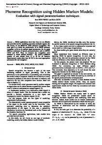
In this paper, we present an algorithm that segments a piece of music into a succession of abstract textures over time. Like a MIDI score, a musical stream can be described as the superposition of different sources –i.e. instruments- emitting sound at the same time, each with its own timbre. In this work, “texture” is defined as the composite “polyphonic timbre” resulting from instruments playing together. (Identically, a texture can be viewed as the “monophonic timbre” of a composite meta-instrument). Figure 1 shows an example of instruments merging into such textures. This process is similar to audio segmentation. Segmenting acoustic data refers to identifying and labeling its different sections of interest. For instance, if we process music, we would like to highlight the alternation of chorus and verse, the beginning of a solo, a sudden change of orchestration, etc. Tzanetakis in [1] stresses the importance of segmentation for Audio Information Retrieval, where it is better to consider a song as a collection of distinct regions than as a whole with mixed statistics. By discarding any pitch and

Figure 1: Comparison of the classic MIDI track representation of music (A) and the texture representation (B). To uncover the different textures occurring in a musical piece, we investigate the use of Hidden Markov Models (HMM). Over the past 20 years, HMMs have been applied with great success to many pattern recognition applications, such as speech recognition, and see

AUCOUTURIER – SANDLER

growing interest in the music analysis community ([2], [3]). In our case, we believe that each state of an appropriately trained HMM can account for a specific texture. The paper is organized as follows. In section 2, we discuss the most relevant signal processing front-end for the model. We examine three methods of spectral envelope estimation: cepstrum, linear prediction and discrete cepstrum, and suggest two ways to encode the resulting feature vector. Their qualities are compared. In section 3, we present an efficient algorithm to uncover the succession of textures using a HMM. We compare the performance of the different front-ends suggested in section 2. We also address the main limitation of the system: its fixed topology. Finally, in section 4, we justify the use of a HMM compared to more static clustering schemes, such as k-means clustering. We show that we often have to take account of the dynamic evolution of the features to achieve a good segmentation.

SEGMENTATION WITH HMM

instrument; namely, its timbre. If we identify the filter' s spectral magnitude and the spectral envelope, it is clear that the envelope is independent of the pitch: the harmonic partials slide along this constant spectral "frame", which determines their amplitude. Thus, in this simplified framework, an "evaluation" of the spectral envelope appears to be a good candidate for the front-end of our system, as it meets our 2 criteria: it is a pitch-invariant measure of timbre. One issue raised by this paper is whether this monophonic model is portable to the polyphonic, multi-instrument context that is of interest for us. A polyphonic texture can be represented in the former framework as a sum of source-filter paths. Using the same model to describe the whole process in a global way then means that we make the following approximation: "We can find a composite pitch excitation U C and a composite metainstrument envelope

i

× U i = SC × U C

(1)

i

2.1- Requirements where It is of great importance to select an appropriate set of features as input to the hidden Markov model. To allow an efficient segmentation of the audio data, the features should meet the 2 following criteria: a) The ideal feature set will be a perceptually realistic measure of the similarity of timbres. Similar textures must be represented by close "points" in the multi-dimensional feature space, and, the other way round, close points should represent similar timbres. b) At the same time, since we don’t want to segment the different notes or events within a single texture, the feature set should be relatively independent of pitch.

S C such that:

∑S

2- FRONT END

Si

and

U i are

the filter responses and excitations of the

individual instruments.”, which seems analytically awkward. Yet, looking at polyphonic spectrums like in figure 3 and 4, we see that this approach, approximate as it may be, may well be fruitful. Envelopes can be defined, and they seem to differ sufficiently from texture to texture.

To assess the quality of a feature set given this compromise between timbre and pitch, we use two specially recorded audio samples. Sample1 is a 5-second clarinet glissando, comparable to the one opening G.Gershwin’s “Rapsody in Blue”. It is an example of a constant texture, with varying pitch. Sample2 is 5-second C4 note generated by MIDI, in which the instrument playing the note changes each 500ms: clarinet-bassoon-trumpet-organ-violin-piano-etc. It is an example of a varying texture with constant pitch. A quality measure of the feature set is obtained by comparing the standard deviation of the features computed on both samples: a good front end would show great variance on sample2, and little on sample1. 2.2- A good candidate: the Spectral Envelope.

Figure 3: superposition of 50 successive STS (30 ms frames) for a polyphonic texture {guitar + bass + synthesizer}

There has been a substantial amount of research on timbre and instrument separation, in most of which the analyzed acoustic data consist of short monophonic samples of a simple instrument. In such a context, it has been demonstrated that a large part of the timbre of instruments was explained by their spectral envelope. The spectral envelope of a signal is a curve in the frequency-magnitude space that "envelopes" the peaks of its short-time spectrum (STS). [4]. This echoes a classic model for sound production, in which the observed data results from a source signal passing through a linear filter. (Figure2).

Figure 2: the source-filter model of sound production. Although it has been designed to model speech production, it is also partially valid for musical instruments: in this case, the source signal is a periodic impulse drive responsible for the pitch, and the filter V(z) embodies the effect of -say- the resonating body of the

Figure 4: superposition of 50 successive STS (30ms frames) for a different polyphonic texture : {piano + bass + synthesizer}

AES 110TH CONVENTION, AMSTERDAM, NETHERLANDS, 2001 MAY 12–15

2



To estimate the spectral envelope of the musical signal we analyze, we consider three different schemes: 2.3- Linear Prediction (LP) This makes full use of the source-filter model as it identifies V(z) as an all-pole filter of order p.

V ( z) =

1 1 + a (1) ⋅ z −1 + ... + a ( p ) ⋅ z − p

(2)

As described in [5], we first estimate p+1 autocorrelation values for each frame, and then derive the p filter coefficients from a set of linear equations. This involves inverting the autocorrelation matrix, which is done with the Levinson-Dublin algorithm for Toeplitz matrices. From the p coefficients, we then have access to the spectral envelope of the filter (Figure5).

Figure 6: Comparison of the standard deviation of LPC coefficients on sample1 and sample2, plotted against the number of coefficients

If we consider the signal to be produced by the source-filter model, then taking the log-spectrum exhibits a deconvolution of the excitation and the envelope.

log(V ( z ) × U ( z )) = log(V ( z )) + log(U ( z ))

Figure 5: Spectral envelope estimated via LPC, order 15.

(4)

Thus, the lower cepstral coefficients account for the slowly changing spectral shape, and the higher orders describe the fast variations of the excitation. So, to obtain an envelope measure that is independent of pitch, we should only use the first few coefficients. (Figure7). Note that the low order cepstrum can be roughly viewed as averaging the spectrum: it no longer has the property to envelope and link the peaks of the STS.

The linear prediction coefficients (LPC) a(i) control the position of the poles of the transfer function: this method is thus appropriate for modeling a signal with significant peaks in its Power Spectral Density (PSD). Since it assumes that the excitation is a white noise, the spiky aspect of the output’s PSD is also seen on the filter’s envelope estimate: it gets down very sharply in between the partials, rather than linking them smoothly. Figure 6 compares the standard deviation of LPC on sample1 and sample2 plotted against the order of the LPC: the ratio between the two remains approximately constant with as the number of coefficients varies. Indeed, the pitch dependence comes from the “spiky” behavior, and this behavior doesn’t depend on the order. By reducing the number of poles, we just reduce the number of spikes, which simply yields poorer estimates. 2.4- Mel Frequency Cepstrum (MFC) The cepstrum is the inverse Fourier transform of the log-spectrum.

cn =

ω = +π

1 × log( S (e jω )) ⋅ e jω ⋅n dω 2π ω =∫−π

(3)

We call mel-cepstrum the cepstrum computed after a non-linear frequency warping onto the Mel frequency scale. The cn are called MFC coefficients (MFCC). MFCCs are widely used for speech recognition, and Logan in [6] has shown that they were also justified for music analysis. Several instrument recognition systems also make use of MFCC [7], [8].

Figure 7: Spectral envelope estimated with MFCC, order 8. Figure 8 compares the texture/pitch standard deviation for MFCCs: Logically, the low order cepstrum shows a good ratio, being rather independent of pitch. As the order increases, the “sharp” variations of the spectrum are increasingly taken into account, and the ratio progressively falls under 1. The limit point is around 10 coefficients.

AES 110TH CONVENTION, AMSTERDAM, NETHERLANDS, 2001 MAY 12–15

3



Figure 8: Comparison of the standard deviation of MFCC on sample1 and sample2, plotted against the number of coefficients

Figure 9: Spectral envelope estimated with Discrete Cepstrum, order 8.

2.5- Discrete Cepstrum (DC) Both previous methods are spectral estimation techniques, and we examined how they stood up for the problem of spectral envelope estimation. This third method, though, is specific to envelopes. It was introduced by Galas and Rodet in [9], who suggested to estimate the cepstral coefficients directly by interpolating the spectrum. Since we want the envelope estimate to smoothly link the partials, this suggests that we already know the envelope estimate’s value at the partials frequencies: it is the value s k of the spectrum at these same frequencies f k . If we do a careful peak-picking on the spectrum to measure the frequencies of the partials, the (log-amplitude) envelope estimate A(f) can then be interpolated from the corresponding values of the spectrum. In practice, this is done via the minimization of the frequency-domain least square criterion:

ε = ∑ 20 ⋅ log(sk ) − A( f k )

(5)

Figure 10: Comparison of the standard deviation of Discrete Cepstrum on sample1 and sample2, plotted against the number of coefficients.

k

where

the

log-amplitude

envelope

estimate,

A( f ), ∀f

is

parameterized in terms of p cepstral coefficients (if order is p): p

A( f ) = c0 + 2 ⋅ ∑ ci . cos(2πf ⋅ i )

(6)

i =1

Cappe in [10] shows that this method suffers from illconditioning problems, and derives a modified criterion which constraints the envelope to be smooth. The resulting envelope estimate seems to be a good compromise between "good fit to the partials" and "pitch independence". (Figure9) Figure 10 shows the texture/pitch standard deviation for Discrete Cepstrum Estimation. We notice the same behavior than with MFCCs (low-order/high order), only here the variances are globally very small. The estimate is so smooth than it levels the differences between the spectrums.

2.6- Encoding So far, we’ve shown how a vector of LPC, MFCC or discrete cepstrum coefficients can describe the spectral envelope of a STS. In an attempt to improve the texture/pitch ratio of our feature set, we investigate an alternative encoding of the estimated envelope: For computational respects, directly storing a sampled representation of the continuous envelope estimate itself is intractable, or it would imply a drastic down sampling. We can however describe the continuous envelope estimate by computing its moments, as if it was a probability distribution: we get a new feature vector consisting of the curve’s centroid (first order moment), standard deviation (second order moment), skewness (third order), kurtosis (fourth order), and so on. We notice that the standard deviation values with the moment encoding are generally higher than with the coefficient encoding. Figure11 compares the texture/pitch standard deviation ratio for the three methods of estimation (MFC, LP, DC) with the moment encoding. The ratio for MFC and DC is