General Disclaimer. One or more of the Following Statements may affect this Document. This document has been reproduced from the best copy furnished by ...
General Disclaimer One or more of the Following Statements may affect this Document
This document has been reproduced from the best copy furnished by the organizational source. It is being released in the interest of making available as much information as possible.
This document may contain data, which exceeds the sheet parameters. It was furnished in this condition by the organizational source and is the best copy available.
This document may contain tone-on-tone or color graphs, charts and/or pictures, which have been reproduced in black and white.
This document is paginated as submitted by the original source.
Portions of this document are not fully legible due to the historical nature of some of the material. However, it is the best reproduction available from the original submission.
Produced by the NASA Center for Aerospace Information (CASI)
Segmented Testing* John P. Robinson Electrical and Computer Engineering University of Iowa Iowa City, Iowa 52240
ABSTRACT
The fraction of faults detected for a digital network is frequently high for the first few input combinations applied out of a set of test vectors. When the particular ordering of test patterns does not appreciably change the shape of the coverage curve, there appears to be an advantage to splitting the test into segments which are applied at different times. It is shown that the expected time to error detection and the probability of an undetected double error can be reduced. The amount of reduction is dependent on the shape of the fault coverage curve. It is conjectured that such a reduction can be obtained for VLSI networks.
f
(NASA-Ch-173188) SEGMENTED TESTING (Iona Univ. ) 26 p HC A03/HF A01
N84-16855
CSCL 12A
Uncla s G3/64 00533 * This
work was supported by NASA Langley Research Center under SAG-195.
I
1
INTRODUCTION
The shape of a fault coverage curve; i.e. the cumulative fraction of F
detected faults as a function of the number of tests applied, is often a saturated curve. Recent work on fault-tolerant computing (1,2) and built in test (3) have reported such situations. This characteristic is often found in testing situations; fault table minimization, D algorithm, path sensitizing, random test, etc. (4). The basic strategy proposed in this paper is to split up a test set into two or more segments; then apply these shorter tests at differed times so that there is a reduced time between periods of testing. If each test segment ^t
detects many or most faults then it is expected that faults should be detected sooner on the average. Consider the 15 gate combinational logic c3.rcuit in Figure 1. The function realized is a 3 out of 5 select followed by a majority vote. Three ones on the E inputs select three T lines out of the five using f
gates 1 to 5; gates 6 to 11 OR the selected lines in various pairs which are ALNDed at gates 12 to 14. Gate 15 ORs these products to realize the majority of the three selected T inputs. This function was implemented in a RockwellCollins gate array as part of a VLSI project. Suppose the possible faults are single gate input or output stuck-at faults. There are 3 leads each for gates 1 to 14 and 4 leads for gate 15. The 46 total pins result in 92 single faults. Since there are no reconvergent fan-out paths of differing inversion parity, expanding and contracting faults can be considered separately. We start with tests for expanding faults. It is easy to show that the following 4 tests will detect all combinations of gate input or gate output stuck faults which increase the number of ones in the function.
T
I
Y
T
T,
El
Figure 1 Gate example
..J
I
2
T11 E - 11100 T - 01011
T 12 E - 00111 (1) T - 11100
T 13 E - 01011 T = 11100
T 14 E - 11100 T - 00111
Any single test from set (1) will detect 27 of the 46 expanding stuck faults while any two consecutive tests (including T 11 , T14) will detect 44 of the 46. For contracting faults the following six tests will detect gate input or output stuck faults.
T01
E = T = 10010
T02
E - T = 00101
T03
E = T = 01001
T04
E = T = 01010
T05
E = T - 11000
T06
E = T = 00110
(2)
The first 3 tests detect 40 out of the 46 contracting faults.
3
Suppose we interlace sets (1) and (2) as follows:
T 110 TOI , T 12 , T02 , T039 T 139 T0O T 14 , T0P T06
(3)
It is easy to count the number of single stuck faults detected by (3) as individual patterns are applied. The resulting fault coverage curve is given as the solid line in Figure 2. Rotating (3) and considering other initial test patterns gives the other two curves in Figure 2. Next we compare two different methods of applying set (3): 1.
Complete Test: The entire set (3) is applied every I time units,
2.
Segmented Test: The first 5 tests of (3) every odd multiple of I/2
time units and the last 5 tests of -(3) every e9en multiple of I/2. In the complete case any single fault in the first I time units is detected by the test at time I. We ignore faults which occur during the testing for the moment. This assumption does not significantly change the result. Suppose further that the fault process is stationary. The expected time to fault detection ETFD is thus half the interval or I/2. For the segmented case consider single faults that occur in the first internal of I/2. Some faults are missed by the five tests at I/2 and are not detected until the end of the next I/2 segment by the remaining five tests. For this example it turns out that the same fraction of faults in the second subinterval are missed by the even set. The faults detected by the odd set will have an average time to detection of half the subinterval or I/4. The 11 faults missed by the odd set will have their time to detection increased by I/2, the time between the odd and even subtests.
I
ORIGINAL PAGE ;S OF POOR QUALITY faults detected
100%
50%
0% 2
4
6
8
10 tests
Figure 2 Coverage curves for gate example
Rti
Gy" 4
fault detection fir this
ETFD : 92 + (
4 + 2
)
92
(4)
s
1 57 2 92
The second factor of (4) is a factor by which we have reduced the ETFD by partitioning the complete test into two segments. This reduction is bought.at a cost of testing twice as often. The overhead in shifting to testing mode has been doubled. 4
Another measure of testing goodness applicable to fault tolerant system
-^ s
F
is the probability of an undetected double error. The idea is that a single fault tolerant system can either adapt or flag the rest of the world when a single error is detected yet still compute correctly. Undetected double errors on the other hand might lead to overall system failure (1, 2). We assume a Poisson fault process (5) to estimate the probability of an undetected double error. For a Poisson process with rate a, the probability of exactly k occurrances in time interval t is
p(k,t) - e -Xt
(at )k
(5)
k!
i
To simplify the example we assume that at is very small so that
a-at
can be
treated as the value 1. This assumption does not appreciably change the character of the results. Expression ( 5) thus is reduced to
5
(Xt)k
p(k, t ) -
(6)
k!
Also we note that p(k,t) is much larger than p(k+l,t), i.e. single errors are much more likely than double errors which in turn are much more likely than triple errors, etc. Consider P 21 the probability of an undetected double error in an interval I between complete test sets. For L successive frames of I this probability . is approximately
P - L (aI)2 2
(7)
2
Expression (7) assumes that LXI is-small compared to 1. Next consider the complete test divided in two and applied every I/2 time units. Double errors within the shorter interval I/2 are undetected. In addition some single errors in the first interval are undetected after the partial test at I/2. If such an undetected fault is followed by another fault in the next interval before time I then an undetected double error has occured. In a similar fashion there are some single errors between time I/2 and I which when followed by another single error in the next half interval result in an undetected double error. Note that these cases are in essence the same as those in the discussion leading to expression (4). Adding the probability of these three situations for L frames of I we find a total probability F
'^
P2 ,y
LW
L
(aI) 2 2
11
L-1 11
[1 + q 2 + L 92^
(8)
i t
6
Replacing ( L-1) in the last term of (8) by L simplifies the expression with the following upper bound.
P2 = L
"2) 2 (.1)
(1 .. 92 + 92)
(9)
The particular arrangement of (9) is intentional. The form is extended to the general case in the appendix A. The left most portion, L(XI) 2/2, is the probability of the complete test ( 7). hex... the 1 / 2 term corresponds to one over the number of segments. Finally, the right -most term is 1 plus twice the fraction of undetected faults. Comparing ( 9) and (7) wt see that the segmented test probability is reduced by a factor of (57/92).
__ ,^.
7
GENERAL CASE
In appendix A expressions are developed for the mean time to fault detection and for the probability of an undetected double error when segmented testing is used. Each of the M test segments is assumed to be applied at uniform time intervals. The extension to nonuniform application is straightforward and could be advantageous in some cases. The forms of these expressions allow a segmenting gain to be defined, assuming the same average testing effort for segmented and for nonsegmented test. This gain g(M) is the ratio of the probability for the segmented to the nonsegmented case. For both mean time to detection and probability of an undetected double error, the same gain expression results,
M-1 g(M) - M/[1 + 2 E ai^
(10)
i=1
The parameter M is the number of O!st segments and a sub i bar denotes the fraction of faults missed by i consecutive test segments averaged over all M starting positions. If the coverage curve is a straight line, then it is easy to show that the gain is always 1. In this case there is no advantage to segmenting. When the curve is concave (e.g., where there is a lot of initialization of state variables in a sequential network) then the gain is less than one and segmentation makes things worse. Fortunately the convex shape seems much more prevelent and improvement is often possible. Examining the gain expression (10) we see that the numerator and denominator bo;:h increase with M. Whether an optimum value of M exists depends on the coverage curve. Practically speaking one would expect test
t1 tt^^
(1^ f.7('^} `
.. Ems!
overhead to eventually become significant as M is increased. In addition, M is limited to the number of individual tests in the complete test T. With E r
these factors in mind it is instructive to consider the theoretical case where the coverage function is an exponential. Let
ai =
1(11) 2 M
When the number of faults times some a t is less than one we assume that the test is complete. Using (11) in (10) and letting i become large will merely lower bound the possible gain. Substituting (11) into (10) we obtain a lower bound on g(M),
M(2 K/M— 1) (2K/M+ 1) .
(12)
Supposing that M is a continuous variable and maximizing (12) with resnect to M we find that the maximum occurs for M very large and that
Lim g(M) = In 2 K 2
s or approximately
g
0.34657 K
(13)
we let g denote the unrealizable gain maximum. M larger than the number of tests has no meaning. For M
g(K/2) = 0.3 K
K/2 in (12),
(14)
9
and
g(K/2) - 0.8656 g.
For the gain to be half of g we find Numerically that
M
L 5.525
Example 2 Suppose that a network requires L = 48 tests and that the coverage curve satisfies (11) with K - 12. the limiting value for the gain g is 4.159. When M - 6 there are 6 subsets of 8 tests each and the a coeficients would be
1
a1 = 4 i
Any 8 test segment detects 3/4 of the faults. The gain from (12) or (14) computes to
g(6) = 3.6
Evaluating (10) directly assumeing a
is zero for i > 5 gives
g(6) - 3.601
Table 1 lists the gain function for example 2 as a function of M.
^iil j
of 10
M Number
g(M) ImprovL-aent
of Segments
Ratio or Gain
2
1.998
3
2.647
4
3.111
6
3.601
12
4.000
24
4.118
48
4.149
Table 1. Gain for Example l
s
4
Q.
e
a 11
Case Study
The segmented testing idea was applied to a particular subsystem of SSI and MSI logic called the bus guardian unit (BGU). A brief description of this subsystem and the testing assumptions are given in 9ppendix B. The unit has a complexity of 1296 equivalent gates and 655 packag- pins. Assuming single pin stuck at 1 or 0 faults, a lower bound on the fraction of missed faults was made for M=6. From these estimates (Tables B1) we can compute a lower bound on the segmenting gain (expression 10) for 2,3 and 6 segments (Table 2). it is felt that these lower bounds are within 10% of the actual valves for the test set considered.
x
.:J
ay 12
M Number of Segments
g(M) Improvement Ratio or Gain
2
1.49
3
1.79
6
2.22
Table 2. Segmenting Gain for the Case Study
v
i 13
DISCUSSION
The segmenting of a test set presented may also be applied when a processor is tested by executing self—test code. Segmenting should be i
beneficial whenever the overhead associated with switching to test mode is small and little initialiation is associated with test subsequences. It is possible to specifically design test sets to enhance the gain obtained from segmenting. Examples have been constructed where a slightly longer test which is constructed to be segmented yields a lower mean time to detection than the shortest test set. In both cases the average number of tests per unit time was held constant. Finally it may be possible to design networks to maximize the gains from a segmented testing environment.
F^
14
REFERENCES
1.
S.J. Bavuso, "Advanced Reliability Modeling of Fault-Tolerant ComputerBased Systems," NATO Advanced Study Institute, Norwich UK, July 1982.
2.
A.L. Hopkins, Jr., T.B. Smith, and J.H. Lala, "FTMP -- A Highly , Reliable Fault-Tolerant Multiprocessor for Aircraft," Proceedings of the IEEE, pp. 1221-1239, Oct. 1978.
3.
B. Konemann, J. Mucha, and G. Zwiehoff, IEEE J. Solid State Circuits, Vol. SC-15, No. 3, pp. 315-319, June 1980.
4.
Z. Kohavi, Switching and Finite Automata Theory, McGraw-Hill 1970.
5.
E. Parzen, Modern Probability Theory and Its Applications, John Wiley, 1960.
Al
In this appendix we develop expressions for the probability of a double error occuring before the first error is detected, P 2 , and the mean time between single fault occurrence and detection MTFD. The fault process is assumed to be Poisson with the fault rate a very small. Initially suppose that a complete fault detection set T of length L is divided into M segments and is applied to a unit under test uniformly spaced in time and repeated periodically. The total time for one complete test is denoted by I. The fraction of time actually spent applying test patterns is assumed to be small. If not, the results are not changed significantly but the analysis is considerably more complex. Let T
denote the jth test
segment. The total test T is then
T as T T 1 ... T M-1 , 0
(Al)
Any rotation of T, e.g.,
T
Tj+l
TM-1 T0T1
(A2)
Ti-1
is assumed to also be a complete test and to have the same coverage curve as T. This is for simplicity of notation and will be relaxed later. Let aj denote the fraction of faults which are undetected by the first j test segments. Clearly a
is nondecreasing in J. Figure Al indicates a
typical coverage curve.
on a
ORIGINAL PAGE 19 OF POOR QUALITY
.R
100%
0% T 1 T2
Figure
Al Coeficient
0C
T. J
Tests
for a coverage function
a
OR IGINAL PAGE [.9
A2
OF POOR QUALITY For a Poisson process the probability of exactly k occurrences in a time
t is given by
e -at (Xt)k
(A3)
k!
where a is the rate parameter. Consider the system for L complete testings. In this total time there are LM intervals between test segments. Consider the instances where a single error in the first interval is undetected before some other error occurs. A double error before any testing has probability _ XI 2 M ( e ^M ) 2 •
(A4)
We suppose that XI is very small compared to 1 so that the exponential term can be replaced by 1 in the various expressions. Thus a double error in the first interval has probability given by
(
XI)2/2M2.
A single fault in the first interval which is missed by test segment To has probability al
XI
assuming equally likely faults. A single fault in the
I . This situation has probability second interval has probability^' a (),1)2 In a similar fashion an error in the first block which is 1 M2 undetected in the first j intervals followed by an error in interval j+1 has probability a. (X2)2 M In the LM intervals the first case occurs LM times, the second occurs LM1 times, and the last occurs LM -j times. Adding all such terms results in the probability of two errors in an interval or a single error which is undetected before a second error occurs, P2 A a
1
A3 ORIGINA L
P" CZ: 13 OF POOR QUALITY 2)2 [^ + a l (LM-1) + a 2 (LM-2j + •• + a j (LM-j) ••] _
P2 M
(XI) 2 LM M-1 2 + E aj(LM-j)] M 2 [ j =1 2
M-1
P2 = L(MI) [f 1 + J E
aj(1 -)]
tA5)
For L large we can replace (1- M) by 1 and approximate this expression by
M-1
2
P 2 = L(MI) [
2
+ E a
i]
J=1 M-1
2
P L(^2)2
1
E
(1 + 2
Expressions (A5) and
a.
(A6)
.
j=1
( A6)
omit triple and higher order faults since we
have assumed that XI is very small.
The first factor L(XI) 2 /2 is the
._4 .
probability of two errors within an interval I for L intervals. case where the total test is applied once in I time units.
This is the
The factor 1/M is
the maximum reduction possible for M segments when the coverage curve is very steep, i.e., the sum of the 61 is small.
The last term is the dependency on
the shape of the coverage curve. Next suppose that a rotation of the test set (A2) gives a different coverage curve than the initial order (A1). probabilities could result.
Up to M different fractional
But in our summation leading up to (A5) we can
replace a l by the average of the M possibility different fractional coefficients, one for each phase of (A2).
Thus we define an average
fractional coefficient aj, 1 M-1 aj
M
E fraction of faults undetected by Ti T i+1 Ti+j-1 1=0
L
A4
ORIGINAL PAGr, IS
OF POOR QUALITY '
where the subscripts are added modulo M. Using the same procedure as led to (A6) we find the probability P2,
P a L(aI) 2 1 (1 + 2 M E l nj) 2 ^— M j =1
(A7)
The computation of the mean time between single fault occurrence and
s
detection, MTFD, is quite similar to that of P 2 . Suppose initially that any rotation of T has the same coverage curve. A fault can occur uniformly within the first interval I/M. For those faults that are detected by T o the mean Y
time is just half the interval or I/2M. The fraction of such faults is i
1 •- a l . The fraction a l - a 2 of faults in the first interval is detected by T i . For this second class the mean time is I/M longer or 3I/2M. Forming the expected value we find
MTFD = 2M [(1 — a l ) + 3(a l — a 2 ) + 5(a
M-1 =ZM[1+2 E
^J
2
— a 3 ) + •••]
(A8)
j=1
Again the interpretation of (A8) is similar to that of (A6). The factor I/2 is the value expected for no segmenting, the second factor 1/M is the maximum conceivable reduction for M segments, and the last factor is the coverage curve coefficient. As was the case for P 2 (A8) is easily extended to different coverage curves for rotations and
M-1 jE l MTFD 2 M [1 + 2 aj ]
(A9)
B1
I
Appendix
B -
Case Study
Introduction
The bus guardian unit
(BGU)
of the fault-tolerant multi-processor (FTMP)
is specialized module designed to enable or decouple a bus drive to a system bus line.
Two
BGU's
are used for each processor/memory unit.
equivalent complexity of about 1200 logic gates.
A
BGU has
an
In operation, 3 out of 5 bus
lines are selected on the basis of an internally stored select code SEL.
Each
selected bus line is input to a synchronizing sub-unit called a deskewer.
The
three synchronized bit streams are voted to yield a serial message. message is recognized as being addressed to the particular storage registers are updated.
BGU,
if the
then one of 5
Four of these registers generate the 20 BGU 1
output enable lines while the fifth register contains the select code, SEL. 1 8
Because of the fault-tolerant nature of the communication scheme and the limited output visibility, the BGU is an interesting module to test. simplify the discussion we will ignore the specialized
BGU
$.,
To
`:~
operations
associated with power-on, master-resest, and power-fail and consider normal d operation. At the highest level there are 3 types of Case 1.
Correct response to a valid message,
Case 2.
Failure of the
Case 3.
Change by the
BGU
BGU
behavior;
to recognize a valid message, i
BGU
when not commanded.
These last two correspond to a miss or a false alarm respectively. cases require separate tests to detect.
These
The following three facets of the
BGU
add to the testing problem.
{i
M
B2
The FTMP communication system is designed to tolerate single failures, hence the three seperate serial inputs which are voted. But with three correct bus inputs, many BGU interval faults are also tolerated when they occur prior to voting. BGU voter discrepencies (2 of 3 or 1 of 3) are not visible as outputs. This situation requires test inputs which are also 2 of 3 or 1 of 3 to propagate faults to a visible output. Closely related are input selection faults. The 3 of 5 select logic and SEL code assignment interact. Many single bit changes in a SEL code result in 2 of the three desired bus inputs still selected. Thus many select logic faults and SEL register faults are not visible with 3 correct inputs. Since the SEL register contents can only be infered from other register outputs, a series of tests are needed. Finally the BGU address decoder utilizes 20 message positions. A single stuck position at the correct value can occur in 20 ways, hence 20 tests are needed to detect these Case 3 failures. In addition there are other faults associated with the BGU tima_ng logic which result in Case 3 behavior which can not be overlapped with addressing false warm faults. To illustrate the segmenting idea we make the following testing assumptions. The assumptions 2 and 3 correspond, approximately, to the manufacturing test environment. 1.
The fault class is single pin stuck-at 1 or 0 faults.
2.
The 5 system bus lines are available as inputs. Bus inputs can be freely chosen.
3.
The 20 enable ouputs are observable.
4.
Fault dectection is the objective. The BGU is constructed from 50 digital integerated circuits (Table B1), 3
delay units, two op amp comparitors and some discrete components such as pull-
tM B3
up resistors, decoupling capacitors, etc. The unit is assembled on a single circuit board. The digital circuits include 26 SSI packages, 24 MSI packages, and 3 delay units. The SSI accounts for 327 logic pins with 193 equivalent gates; the MSI for 328 pins with 1103 equivalent gates. As compared to LSI or VLSI the gate to pin ratio is quite small.
h
mm ^
-^
p^ ORIGINAL ^^^^^^ wF POOR QUALITY
^
84
ot i,^
Description Kna 6 p teE
Yrs
FinE Get*s
54L500
Quad NAND
12
4
2
^4
54LS0Z
Quad NOR
12
4
1
12
54L604
Hex Inverter
12
2
}
:2
540 4
Her inverter
12
54LSO9
Quad AND-OC
12
54LS1O
7ripIe N.kND
12
54LS30
8 input NAND
54LS32
Quad OR
12
4
2
24
8
54LS74
Dual D F>ip-Flop
12
12
7
84
84
14
16
1
14
1 !,
1E:
10
1
18
10
54LS112 Dual J-K Flio-Flop 54LS240 Octal
Buffer
8
12 4
4001G
Quad CMOS NOR
12
4
2
24
8
700,
He,C1OS Sufier
14
7
5
70
A
327
193
14
16
4S
208
70
29O
42
51
2G
S 2:
42
174
5ubto01 ^^
54LS138 3-G Decoder 54LAW Lctal
8-1 Mux
54LS253 Duel 54LS259 Octal
^
12
Shift Regs
54LE1P1 4 Bit Up/Down Ctr 54LS251
1^
4-1 Flux
10
5S
1.4
17
14
it
5
I
Latch
7136
6 Bit Commarator
14
22
1
14
22
540174
Hex Register CMOS
14
62
5
70
SlU
'
Subtota!
328 11O3
Total Pins = Logic Pins
55 12&t-
Gates'= Eouiva.l*nt Gates
Table Bi- Bus Guardian Digital
Integrated Circuits
B5
Examining the design 11 detail there are five key areas which require particular test inputs: A.
The five output registers and associated tri-state buffers.
B.
The address d`coder.
C.
The select code register and 3 of 5 select logic.
D.
The two vvicers.
E.
The timing decade logic.
r.
Area C has ten distinct paths through the select logic which require two messages for each path, one to change the SEL code and a second message to
i
verify the updated SEL code by changing an observable output. Another five messages are required to complete the tc G ting of area A. Area B re q uires 20 test messages for Case 3 (false alarm) failures as noted earlier. The BUSY voter in Area D requires 6 additional false alarm messages. Finally Area E can be tested fog Case 3 faults with 7 more Y
message. The total set of 58 messages is sufficient to test for single pin s-a faults. It can be shown that at least 54 messages are necessary. The sufficient message set can be divided into 6 segments
with each
of
the previously mentioned subsets as evenly as possible yielding 9 or 10 test messages per segment. A^. upper bound on the a
values for this segmented test
set can be determined by counting the number of faultF that are always detected. Exact values could be det%rmined by simulation. From upper bounds on the a
a lower bound on the segmenting gain g(6) expression 10 can be
found. The follo p ing table lists these values.
(b.
B6
i 1
0.29
2
0.23
3
0.17
4
0.11
5
0.05
Table B1. Miss Fractions a
for the Case Study