minimal description length is described in 8]. Segments. The \atoms" from which the waveforms will be composed of are called segments. A segment.
Segmenting and Compressing Waveforms by Minimum Length Encoding Daniel Keren
Ruth Marcus
Michael Werman
Dept. of Computer Science The Hebrew University of Jerusalem 91904 Jerusalem, Israel. Technical Report 89-11 June 1989
Abstract
The paradigm of minimal length encoding is used for superior segmenting and compressing of waveforms. These methods sre shown to be applicable also for segmenting and edge nding in pictures.
0
Introduction Minimal length encoding as a way of describing and explaining information has a long history. William of Ockham in the 14'th century already gave forth the principle known as Occam's Razor Principle; Entities should not be multiplied beyond necessity. The idea of the principle is; of all possible consistent descriptions of an object always pick the shortest description. This principle has been much used since then resulting in shorter and easier to explain or compute theories. In computer science and statistics this idea is known as Kolmogorov complexity. It has also appeared in Valiant's learning theory and Rissansen's minimum description length principle. For more uses, history and references see [4]. In this paper we show how to use this paradigm in order to segment waveforms into meaningful simple parts. These simple parts are the atoms of the waveform, so that if they can be encoded by a short description. We not only have a good segmentation of the waveform, but also a succinct encoding of it. We also show some results using these one dimensional segmentations for segmenting two dimensional pictures. Segmenting waveforms has been treated in [6, 7] and a speci c type of segmenting pictures using minimal description length is described in [8].
Segments The \atoms" from which the waveforms will be composed of are called segments. A segment is a member of a parametric family of functions F = ff g, usually, in our studies, polynomials or trigonometric functions. For example, the parameters of a polynomial will be its degree and coe�cients. Given a set of data points, fx ; y g =1 , we wish to describe them as a segment, which is a single member of a parametrized family of functions restricted to the interval. For most sets of points and most nite parametric families of functions, there is no member f of the family such that f (x ) = y for all i. Also, since noise might have been added during measurements, it is not always desirable to nd such a function anyway. To overcome this problem a segment is de ned acceptable if it approximates (in some norm) the given set of points, approximation as opposed to interpolation. A possible such norm, which is used in this paper, is given by the �2 distribution, which gives a maximal likelihood estimator. If we look for the member f of F that approximates the set of points in the least-square sense, we can use the quality of t of f to the data to compute the probability that the data originated from a member of F . The probability is computed using the incomplete Gamma function which also depends on the number of degrees of freedom of F . Thus, the acceptability of a segment is translated to setting a threshold on the result of the incomplete Gamma function; as the threshold is lowered acceptability becomes harder. The computation of the best approximation f is done using least-square and pseudo-inverse techniques. Other possible methods are the use of di�erent criteria for goodness of t such as such as maximum absolute deviation, sums of absolute deviation, xed tolerances or robust statistics. For a review of the above mentioned mathematical techniques and algorithms, see [5, ?]. t
i
i
n i
t
t
i
i
1
Figure 1: Segmentation with a family of Polynomials: There are 40 points composed of four segments and contaminated by Gaussian noise. The dots correspond to the data and the lines to the tted polynomials. There are four polynomial segments: (from left to right) second order, rst order, constant and rst order. The costs of the four segments are: (from left to right) 5,4, 3 and 4. The total cost of this waveform is 16.
Waveforms A waveform is de ned as a concatenation of acceptable segments, so that it is usually only piecewise continuos. This de nition is not unique; Indeed, one can choose every single point (x ; y ) as a segment. This is of course not desirable as it carries no information about the structure of the data. The opposite extreme is to t all the data with one member of F - however, in the case of polynomials this will usually result in an approximation of very high degree which oscillates considerably between the data points; This is the result of trying to t one function to a data set which should be composed of several di�erent parts. Thus it is needed to choose as few segments as possible and of a simple form. In order to do this each segment is weighted according to it's complexity (which in the case of polynomials is an increasing function of the polynomial's degree), and is the minimal information needed in order to encode it. We want is to nd the minimal weight description of the waveform. 1 De ne the digraph G = (V; E ), V being the set of acceptable segments and (v1 ; v2) 2 E whenever the smallest x-coordinate of v2 is immediately after the largest x-coordinate of v1 , and weight the vertices V by the cost of encoding the corresponding segment. A minimum length encoding of the waveform is then equivalent to a minimum weight path in G, the weight of the path being the sum of the costs of encoding each of the corresponding data points by an acceptable segment. Figure 1 is an example of the segmentation process where F is a family of polynomials. The cost of encoding each acceptable segment with a polynomial is the sum of encoding the length of the segment, the degree of the polynomial and its coe�cients. ? � Computing �2 and the best tting segment for each of the P2 intervals takes no more than P P 2 P 2 P 2 O(n ) time as they are both functions of the smaller moments, x ; y ; x ; y ; x y ; � � �, of the data points. This follows from the fact that knowing the moments for the points from i to j it only takes constant time to compute the smaller moments for the points from i to j + 1. Also i
i
n
i
i
i
i
i i
Encoding is done by listing all n elements and using log(n) bits for each element or in the in nite case using a pre x code which takes log(n)+loglog(n)+logloglog(n) � � � to encode n. 1
2
computing the smallest weight path takes similar time. This is true for the worst case, but if there are not many long segments that are acceptable segments for the given data the whole process can take linear time by not trying to merge two barely acceptable segments into a longer one. 2 I t is known that the data set is composed of k segments, it is then possible to do a binary search in the threshold domain that will result in a threshold dividing the data to the required number of segments. This whole process takes no more than a factor of log(n) more than the ordinary algorithm.
Compressing Waveforms
Using the previous algorithms we can compress waveforms. This will be a lossy compression but it will be close to the original data in whatever criteria we chose for similarity between data and its describing segment. Thus in order to represent the data after it is segmented only the parameters and length of each segment are needed. In cases where the waveform has some structure that is describable by members of the parametric family, good compression can be achieved.
Comparison to Other Methods
Two other approaches of segmenting waveforms are sub-division and edge detection. In the subdivision approach [7], one tries to t a member of F to the data. If this fails, the data is divided and the attempt to t is continued recursively. When this is done, a merging stage is run in which similar segments are merged according to some acceptability criteria. In the edge detection approach [3], an edge detector of some kind is applied to the data and the segments are determined by the resulting edge points. A drawback of the edge detection approach is its locality; The edge detector might break a segment in the middle because of a small disturbance due to noise that would go by unnoted by the algorithm described which is more global in nature. A drawback of the sub-division approach is in the splitting process which is usually not consistent with the structure of the segments. Also, none of these approaches is guaranteed to nd a representation which is minimal in some sense. Figure 2 shows the sub-division method. The data is always split into two parts when the t fails. Another popular segmentation approach is based on thresholding, but it is not suitable for the case of waveforms as the segments are not constant, and so thresholding can break a segment into many pieces.
Multi-Scale Decomposition as Degree of Acceptability
In the segmentation algorithm described it was noted that the result depends upon the threshold of the incomplete Gamma function used to test the probability of the data originating from a member of F . By changing this threshold we get a hierarchy of representations that are closer and closer to the data but containing more segments and more costly to encode. Figure 3 shows the di�erent segmentations resulting from the hierarchy of thresholds. Figure 4 shows a multi-scale diagram of segmentation using a model of constants.
This whole discussion is true only if each member of the parameterized family of functions has at most some xed number of parameters. 2
3
Figure 2: Comparison of our method to binary sub-division: There are 32 points composed of three segments and contaminated by Gaussian noise. (a) minimal length encoding (b) binary sub-division: threshold of split-merge = 0.35 (c) binary sub-division: threshold of split-merge = 0.3
Figure 3: Multi-scale decomposition: (a) thresh = 0.3 (b) thresh = 0.2 (c) thresh = 0.1 (d) thresh = 0.05 (e) thresh = 0.03
4
Figure 4: Multi-scale diagram: Upper row: Three di�erent examples. Lower row: Multi-scale diagrams of their segmentation with the family of constant functions. The black pixels correspond to borders between segments. Each row of pixels corresponds to a segmentation done according to a di�erent condition of acceptability of the segments. The top row of is when no errors are permitted and every pixel is a segment. The number of segments becomes smaller as the condition of acceptability is relaxed.
Segmentation of Multi-Dimensional Data Sets
The algorithm presented relies heavily on the one-dimensionality of the data set. Our current research is aimed at extending the result to higher dimensions by relating the segmentation of a data set to the segmentation of its projections on lower dimensions. The reason we do not compute the minimum length encoding directly in two dimensions is that it is the class NPC, as the problem of minimal partition is NPC [2]. Projection of a polynomial surface image on one dimension is useful because any intersection of a d'th degree polynomial surface, bivariate polynomial, with a plane is a d'th degree univariate polynomial. Polynomials are suitable, for instance, for the case of optical ow; It is known [1] that planar bodies in rigid motion give rise to optical ow that is a second-order polynomial in the image coordinates. Also, illuminance functions behave many times in a polynomial fashion, and segmenting an image into areas of constant grey-level might fail because even if an object in an image is of uniform color, it's grey level in the image may vary polynomially. Range data of man made objects are often describable as piecewise polynomial of low degree also. Figures 5,6 show the segmentation of grey level pictures. One-dimensional segmentation was done to each row of the pictures.
Conclusions and Further Research
We have shown a tractable minimal length encoding algorithm for segmenting and compressing waveforms and a few uses for it in two dimensional data, namely, pictures. 5
Figure 5: Linear surface segmentation: The background is composed of two constant grey levels. The square's grey level changes linearly from left to right. The image is contaminated by Gaussian noise. (a) original image (b) segmented image. Black pixels indicate a border between two segments.
Figure 6: Linear surfaces segmentation: Image is composed of linear bivariate functions and contaminated by Gaussian noise. (a) original image. (b) segmented image. White pixels indicate a border between two segments.
6
We are currently working on pyramid techniques to speed up computations, the extraction of sub-pixel width information and e�cient heuristics for segmenting pictures using these ideas.
References [1] G. Adiv. Determining three-dimensional motion and structure from optical ow generated by several moving objects. IEEE Trans. on Pattren Analysis and Machine Intelligence, 7:384{402, July 1985. [2] B. Chazelle and D.P. Dobkin. Decomposing a polygon into its convex parts. In 11'th Annual ACM STOC, 1979. [3] D.W.Murray and N.S.Williams. Detecting the image boundaries between optical ow elds from several moving planar facets. Pattern Recognition Letters, 4:87{92, April 1986. [4] M. Li and P.M.B. Vitanyi. Inductive reasoning and kolmogorov complexity. In Proc. 4th IEEE Structure in Complexity Theory Conference, 1989. [5] W.H. Press, B.P. Flannery, S.A. Teukolsky, and W.T. Vetterling. numerical Recipes. Campbridge University Press, 1986. [6] P.V.Sankar and A.Rosenfeld. Hierarchical representation of waveforms. IEEE Trans. on Pattren Analysis and Machine Intelligence, 1:73{80, January 1979. [7] T.Pavlidis. Algorithms for shape analysis of contours and waveforms. IEEE Trans. on Pattren Analysis and Machine Intelligence, 2:301{312, July 1980. [8] Y.G.Lecelerc. Segmentation via minimal-length encoding on the connection machine. In International Conference on Computer Vision, in press.
7