Seismic data modelling using parallel distributed MATLAB

Seismic modelling in parallel M ATLAB

Seismic data modelling using parallel distributed M ATLAB Kayla Bonham and Robert J. Ferguson ABSTRACT Numerical modelling of seismic wave propagation is central to seismic imaging and inversion. Modelling of 3D heterogeneous anisotropic media can, however, simultaneously be both costly and of low fidelity. To address some aspects of the fidelity / cost problem, we present our implementation of seismic modelling within the Rayleigh-Sommerfeld algorithmic framework and implemented in a parallel computing environment. We demonstrate through example, that knowledge of relationships among hardware architecture, support software systems, and resource usage of our algorithm, is of crucial importance to the achievement of worthwhile performance using parallel computing. From an initial, simplistic expression of our parallel algorithm in the M ATLAB system, exhibiting ‘negative improvement’, we incrementally adapt the parallel control framework without losing the clarity or correctness of the original model expression, to bypass successive bottlenecks and achieve substantial performance gains. INTRODUCTION To model high fidelity structural and textural information for large 3D spaces, we are currently in development of a large scale seismic modelling capability. Our effort is based on the Rayleigh-Sommerfeld integral (Ersoy, 2007, p.59) formulation of wave propagation. This is a familiar integral in that conventional imaging by phase shift (Gazdag, 1978) is a special case of this more general theory, and it is unique in that wave propagation is controlled numerically by a set of phaseshift operators, reflection operators, and transmission operators (Cooper and Margrave, 2008). Within this scheme, basically, seismic modelling and imaging are the reverse of each other, and they differ mainly where (and when) data are evaluated during computation (Cooper and Margrave, 2008). In our implementation, a planewave source is distributed over temporal frequency among nodes of our computer cluster. This distribution of monochromatic components of the source wavefield ensures that no internode communication is required until model data are collected and summed – execution is, therefore, “embarrassingly parallel” (Foster, 1995, Section 1.4.4 for example). That is, sets of similar calculations are done with few or no dependencies among parallel computational threads. The hardware system we use is is a cluster computer of 19 nodes, each with eight processors, where each node has common shared memory and local disk storage. The software support system mirrors this, in that we have 96 distributed M ATLAB ‘workers’ enabled on twelve of the nodes, with eight workers to a node. We favour M ATLAB due to its concise notation, comprehensive matrix manipulation abilities, and the fact that arrays of complex numbers are a fundamental data type. Our initial naïve M ATLAB implementation using the built-in parfor construct for the CREWES Research Report — Volume 21 (2009)

1

Bonham and Ferguson

"outer loop" uncovered unsatisfactory parallel performance. By paying attention, however, to both the hardware architecture and the software support system, we have been able to substantially increase parallel performance without disturbing the simplicity of the code (much). HARDWARE ARCHITECTURE ‘Gilgamesh’ ∗ , our Linux-based (Centos 5) cluster, consists of a master node and 18 slave nodes. The master node acts as gateway and network file server to the slave nodes, and all communicate locally by Gigabit Ethernet. The master and slaves have identical system architectures comprising two quad-core Intel Xeon ‘Harpertown’ CPU chips with two-level cache and 16 GB of shared random access memory per node. Each node has 300 GB of temporary local storage space. The master node has 14 Terabytes of disk storage to hold permanent user files and is accessible on all nodes via the network file system. We estimate the theoretical performance of our system in raw CPU cycles to be approximately 1 TFLOPS (1012 FLoating point OPerations Per Second). Gilgamesh exhibits a Non-Uniform Memory Access ( NUMA) architecture at several levels, as do most so-called ‘cluster computers’ composed of network-linked commodity computer systems. This means that the speed of access to particular elements of memory, by any given CPU in the system, depends on their physical and logical proximity across various levels of interconnection that the system architecture imposes. This architecture has both advantages and disadvantages for parallel processing. Use of off the shelf components ensures scalability, and low cost is a definite advantage. A major disadvantage is that, at the application program level, we must pay attention to granularity issues, patterns of memory access, plus network contention among processing threads. SOFTWARE INFRASTRUCTURE M ATLAB is a commercially-available matrix-oriented programming system with a succinct, clear notation in which it is easy to express mathematical and scientific formulae and methods. Within M ATLAB, we use the Parallel Computing Toolkit (PCT) to define extensions to M ATLAB for parallel processing. The PCT provides (among others) language primitives ‘parfor’ (for distributing iterations of a parallel loop among the available ‘workers’ or independent threads of execution) and ‘distributed arrays’ (for allocating slices of a large array among workers, to be worked on separately and combined later). The PCT interacts with another facility, called the ‘M ATLAB Distributed Computing Service’ (MDCS) to provide infrastructure to manage workers across multiple computers. Many M ATLAB operators and toolkit functions are enhanced to automatically detect and make use of PCT, MDCS and multiple parallel workers, if they are present and enabled in a M ATLAB installation.

∗

2

named after the ancient Sumerian hero-king of Uruk, the Beowulf of 4000 B.C! CREWES Research Report — Volume 21 (2009)

Seismic modelling in parallel M ATLAB

APPLICATION The present work is a numerical implementation of scalar wave propagation in anisotropic media in three dimensions according to the Rayleigh-Sommerfeld approach (Cooper and Margrave, 2008). Fundamentally, a source planewave ϕ (z = 0) is extrapolated to a new grid level at z = ∆z according to ϕ (p, ∆z)ω = A (p, ∆z)ω ϕ (p, 0)ω ei ω q(p) ∆z ,

(1)

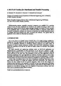
where p = p1 ˆi + p2 ˆj and ω are plane wave coordinates. Amplitude A (∆z) is a reflectivity or transmissivity scalar, and slowness q (∆z) may be anisotropic. To visualize propagating wavefield ψ in three spatial dimensions, for example as a ‘snapshot’ at time t, source planewaves ϕ (0)ω0 through ϕ (0)ωN yq , where ωN yq is Nyquist frequency, are extrapolated to all N depth levels z = ∆z, · · · , N ∆z, and then summed according to X ψ (x, z)t = ε Tp→x {ϕ (p, z)ω } ei ω,t , (2) ω

where ε is a scalar for normalization, and T p→x Fourier transforms ϕ (p) to space coordinates x = x1 ˆi + x2 ˆj. Figures 1a and b are ‘snapshots’ of a point source extrapolated from z = 0 into the subsurface for a fixed time. The medium is homogeneous but anisotropic, so the P- and SV-wavefronts are not spherical (Figures 1a and b respectively). Numerically, each worker in the computer cluster gets a copy of slowness model q (ω, z). Then, monochromatic source ϕω is initialized (a 2D numerical array), and monochromatic wavefield ψ (x, z)ω (a 3D array) is computed through recursive application of equation 1 followed by the Tp→x part of equation 2 and application of scalars ε and ei ω t . The summation step in equation 2 is computed carried separately. To evaluate the performance of our algorithm on our architecture and software infrastructure, a small model space (500 inline / x-line and 250 depths† is chosen. The number of frequencies ω of interest is ∼ 330. Ultimately, we will wish to perform higher-resolution studies to the reasonable limits of the machine. GENERALIZED EXPRESSION OF THE PROBLEM Implementation of the modelling algorithm detailed above consists of two main steps: extrapolation followed by summation. Here, extrapolation consists of initialization of the mononchromatic source plus recursive extrapolation of the source to all z plus scaling, and we represent these combined operations with pseudo-code function A(X,Y,Z,f). Dimensions X,Y,Z represent the spatial dimensions of the 3D visualization matrix, and there are F frequencies f of interest. Rendered in pseudo-code, for f, extrapolation and summation are computed according to Program1:

% Program1 †

A total of 62 500 000 double-precision complex elements in each array ∼ 1 GB each.

CREWES Research Report — Volume 21 (2009)

3

Bonham and Ferguson

init(); R = zeros(X,Y,Z); for f = 1:F L = A(X,Y,Z,f); R = R + L; end final(); where ‘R = R + L’ above is the summation step; Time to execute this function is approximately T1 ≈ Ti + Tca F + Ts F + Tf (3) where Ti is the constant time to initialize the R array and other internal program parameters, Tca is the time to compute function A for one frequency value and return a matrix of dimensions [X,Y,Z℄, and Ts is the time to sum one single-frequency result matrix ‘ L’ into the global result matrix ‘R’. Final time Tf is the constant time to write out the ‘R’ result array and perform other internal program tear-down overhea d. The naïve parallel solution can be expressed as follows:

% Program2 init(); R = zeros(X,Y,Z); parfor f = 1:F L = A(X,Y,Z,f); R = R + L; end final(); where the only difference is the substitution of ‘parfor’ for ‘for’ in the main loop. One might hope for the execution time to be something like T2 ≈ Ti + Tca

F + Tco F + Ts F + Tf , W

(4)

where W is the number of worker processes operating in parallel, and the calculation of all F frequencies is divided equally among workers. Tco is the time to communicate the value of a single-frequency result matrix ‘ L’ back to the main M ATLAB session for summing into the global ‘R’ array. We can’t expect the Tco term to parallelize to the same degree as Tca so the worst-case assumption is that network access will serialize the communications (and summations); M ATLAB’s implementation of parfor, however, is such that as each ‘L’ array is produced, it is transmitted in its entirety to the master session for summation. Contention for the network resource results, plus memory overhead in the master session for buffering the ‘L’ arrays that wait simultaneously to be summed into the global ‘R’ array. With Program2,

4

CREWES Research Report — Volume 21 (2009)

Seismic modelling in parallel M ATLAB

then, we find that the multiple ‘L’ matrices, each as large as the ‘R’ array, become so numerous that they exceed virtual memory of the designated ‘master’ host doing the summation, and execution must terminate. So that virtual memory of the ‘master’ host is not exceeded, Program3 (below), subdivides the F frequencies among the W workers so that each worker performs F/W frequency calculations, and then sums the ‘L’ arrays to reduce the number of ‘ L’ arrays transmitted and buffered to the master session. Then, one of the workers present at a given node is designated as a ‘node representative’ that collects and sums the per-worker local sum arrays ‘S’ into a single per-node sum array ‘ M’ for reporting to the master session and summing into the global result ‘R’.

% Program3 init(); R = zeros(X,Y,Z); parfor w = 1:W S = zeros(X,Y,Z); for f = 0+w:W:F L = A(X,Y,Z,f); S = S + L; end write_file(w,S); end parfor w = 1:W if (iam_node_rep(w)) M = zeros(X,Y,Z); for k = 1:W if (file_exists_lo ally(k)) S = read_file(k); M = M + S; end end R = R + M; end end final(); Although, for sound theoretical reasons, the M ATLAB parfor construct prohibits communication between threads of execution on separate workers, we have bypassed that restriction in a safe way by having workers write their result arrays to the local disk, to be re-read and summed by the designated node_rep worker. The node_rep worker subsequently communicates with the master session to sum its single per-node ‘M’ array into the global result ‘R’. Since communication overhead is a determining factor for overall performance, this ends up being faster, despite the overhead of writing and reading the local ‘S’ files.

CREWES Research Report — Volume 21 (2009)

5

Bonham and Ferguson

Whereas Program2 tried to send all F intermediate ‘L’ result arrays, to the master session for summing, Program3 only needs to send N ‘M’ arrays (one for each node), a huge efficiency gain, at a cost of only (up to) eight ‘S’ arrays written to and read back from the local disks on each of the nodes. The time to execute Program3 is T3 ≈ Ti + [Tca + Ts ]

F W + [Tw + Tr ] + [Tco + Ts ] N + Tf W N

(5)

where N is the number of cluster nodes participating in the computation, and Tw + Tr is the time to write and then read one S array. There is some new overhead in having the workers determine whether they are the designated node_rep for their node (we use the success or failure of an indivisible file ‘touch’ operation), as well as some overhead coordinating the second parfor loop, but these are small, constant overheads which we ignore here. Also, notice that in the second ‘parfor’, all workers but the node_rep have nothing to do; this ends up saving communication time, but one could argue that for the time the node_rep is reading, and summing globally, the non-node_rep workers are under-utilized and CPU cycles wasted.

Program3 has given us quite reasonable performance speedups. The extra control we now have with Program3, over the number of workers per node that participate in the computation, will be quite useful when we increase the dimensions of the problem. At some point, the memory required to contain 8 replicated 3D matrices of the size we wish to use will cause virtual memory contention among the workers. At that time it may be more optimal to specify only 7 or 6 workers per node, and put up with the communication overhead of an extra node or two when summing the final result, rather than risk virtual memory contention causing the computation to thrash on each node. PEER-TO-PEER COMMUNICATION Recently added to the MATLAB version R2008b implementation of the Parallel Computing Toolkit, is the ‘spmd’ construct. ‘Spmd’ stands for ‘single program, multiple data’, which is a computer science term denoting hardware or software architectures in which the parallel processing agents (C PUs, program threads or, in our case, distributed M ATLAB workers), all execute the same program while being given, or permitted to derive, independently varying data objects in their work-spaces. What we did in Program3, with the ‘parfor w = 1:W’ loop variable w governed by W, the number of workers, is to execute the code governed by the loop exactly once per worker. That is exactly what the ‘spmd’ construct would do also. Spmd has most of the same restrictions as parfor on variables local to the loop, but the constraint on peer-topeer communication between workers is lifted. Workers may know their own labindex and may use M PI-derived communication methods labSend and labRe eive to exchange data.

6

CREWES Research Report — Volume 21 (2009)

Seismic modelling in parallel M ATLAB

Rewriting Program3 to use spmd and labSend,labRe eive gives us Program4:

% Program4 init(); R = zeros(X,Y,Z); spmd w = labindex(); S = zeros(X,Y,Z); for f = 0+w:W:F L = A(X,Y,Z,f); S = S + L; end if (mod(w,2) > 0) labSend(w+1,S); else S = S + labRe eive(w-1); if (mod(w,4) > 0) labSend(w+2,S); else S = S + labRe eive(w-2); if (mod(w,8) > 0) labSend(w+4,S); else S = S + labRe eive(w-4); R = R + S; end end end end %spmd final(); This replaces the calls to write_file(my_wID, data ) and read_file(writer_wID) with a pair of calls to labSend(receiver_wID, data_value) and labRe eive(sender_wID), where the worker identifiers xx_wID are obtained from built-in function labindex, or derived from the worker->node distribution scheme. The modulus function mod(my_wID, power_of_two) is a way of determining an order of combination of the local ‘ S’ arrays among the eight workers on a node, in a binary tree pattern, increasing the parallelism of the node-level summation step. The ‘R = R + S’ step still implies serial network communication, and summation into the global result array. Because the labSend and labRe eive operations occur strictly between workers hosted by the same node, communication is faster than between workers on different nodes. The time to execute Program4 is   W F + [Tsr + Ts ] log2 + [Tco + Ts ] N + Tf T4 ≈ Ti + [Tca + Ts ] W N CREWES Research Report — Volume 21 (2009)

(6)

7

Bonham and Ferguson

where Tsr is the time to send and receive one ‘S’ array between workers on the same node. Disappointingly, the version of MPI used by MATLAB uses Unix ‘so kets’ for all communication whether communicating processes are on the same or different nodes, so that copying between workers on the same node is still serialized, as if transferring data across the network, rather than being an instantaneous, direct memory-map operation that theoretically would be possible using the shared virtual memory hardware on the cluster node. Nevertheless, the net result is that the speed of Program4 does improve on that of Program3 by a factor of almost two. A side benefit is a gain in simplicity, where spmd gives us a simpler mechanism to obtain and manipulate node identifiers (e.g. (mod(labindex,8) == 0)), and communication among workers with labSend/labRe eive is much simpler to specify and set up than write_file/read_file that we were forced to adopt when using parfor. PERFORMANCE ANALYSIS

Program3 was run on an unloaded cluster with function ‘A’ and parameters X,Y,Z,F held constant, while run-specific variables W (number of workers participating in computation), and N (number of nodes participating) are varied to evaluate runtime under different degrees of parallelism. The overall elapsed time to compute and write out ‘R’ was observed, and an eye was kept on virtual memory usage on both worker nodes and the node hosting the main M ATLAB session, to ensure virtual memory was not being over-filled and performance degraded by thrashing. Time elapsed, T3 , is plotted for the observed runs in Figure 2. We find that a ‘sweet spot’ exists at about 48 workers on 6 nodes with 8 workers per node – not too many nodes reserved, something close to minimum elapsed computation time of 508 seconds. Slightly shorter elapsed time could be obtained by using more workers, but most of the parallel gains are reached at (48,6). With 48 workers and 6 nodes, half the cluster is left to do a second computation or to let other users make use of the resources. Adding more workers past a certain point, only slows the overall calculation down, because while the computation phase may be quicker, the communication phase where the node_reps report their local sums ‘M’ to the main session, would be increased in duration.

Program4 was run in comparable configurations to Program3, and resulted in a similar scaling behaviour, achieving a run time of 271 seconds using 48 workers on 8 nodes, six workers per node. CONCLUSIONS From a prototype sequential (non-parallel) implementation expressed in M ATLAB, we have gone through several iterations of a parallel implementation, at each step making improvements to unblock one or more ‘bottlenecks’ in performance, taking account of the architecture of the host computer system, the problem structure and algorithm behaviour, as well as the characteristics of the software support infrastructure.

8

CREWES Research Report — Volume 21 (2009)

Seismic modelling in parallel M ATLAB

FIG. 1. Snapshots of extrapolated wavefields in a dipping anisotropic medium. a) P-wave. b) SV-wave.

RTmax = 3875 s RTmin = 508 s Gilgamesh

Runtime (s)

3500 3000 2500 2000 1500 1000

1 2 3 2

4

4

5

6

6

8

7 8

Workers per node

10 12

Nodes

FIG. 2. Plot of runtime versus number of workers and workers per node. Maximum and minimum runtimes are indicated (RTmax = 3875s and RTmin = 508s) respectively, RT for the 8 worker per node configuration of Gilgamesh.

CREWES Research Report — Volume 21 (2009)

9

Bonham and Ferguson

Along the way we stumbled on several ‘tricks’ that gave us some control over the implicit scheduling of M ATLAB workers executing parfor loops within a matlabpool, that may not have been anticipated by the providers of M ATLAB. In the end we achieved a reasonable performance increase, making feasible our investigation of the full-scale problem. We have developed a scheme for analyzing the performance of the program, which will be helpful when considering future improvements and possible re-implementation in a production version. Certain aspects of run-time behaviour are as expected intuitively: applying more processors decreases the time to calculate the per-frequency matrix. The remaining limits to performance speed-up are due to hardware architecture (serial access to the communication channel to report the per-node ‘ M’ result arrays and software support architecture (implementation-specific buffering of entire arrays vs. piecewise result reduction operations, socket-based communication rather than direct memory address space sharing). We found that writing and reading 8 large per-worker ‘ S’ arrays locally, plus communicating a single per-node ‘M’ array to the master session over the local network, takes less time than sending all 8 ‘S’ arrays over the network directly. At the same time it means there is only one ‘M’ array buffered at the master session, rather than 8 ‘ S’ arrays pending summation into the global result ‘R’. A further level of performance was obtained by using spmd instead of parfor, allowing direct communication between workers with labSend and labRe eive. We find that, since the ‘S’ arrays are already in memory, local communication with the designated noderep worker takes place much faster when workers are able to communicate in peer-to-peer fashion. Although the parallel control framework surrounding the computation became somewhat complex during the evolution of the program, the definition of the model (abstracted as function ‘A’) remained untouched and unmodified from its essential expression in M ATLAB, preserving trust in the correctness of the results. ACKNOWLEDGEMENTS The authors wish to thank the sponsors, faculty, and staff of the Consortium for Research in Elastic Wave Exploration Seismology (CREWES), and the Natural Sciences and Engineering Research Council of Canada (NSERC, CRDPJ 379744-08) for their support of this work. REFERENCES Cooper, J. K., and Margrave, G. F., 2008, Seismic modelling in 3d for migration testing: Expanded Abstracts, Can. Soc. of Expl. Geophys. Ersoy, O. K., 2007, Diffraction, Fourier optics, and imaging: Wiley-Interscience. Foster, I., 1995, Designing and building parallel programs: Addison-Wesley. Gazdag, J., 1978, Wave equation migration with the phase-shift method: Geophysics, 43, No. 07, 1342–1351. 10

CREWES Research Report — Volume 21 (2009)